| Issue |
A&A
Volume 534, October 2011
|
|
|---|---|---|
| Article Number | A66 | |
| Number of page(s) | 10 | |
| Section | Interstellar and circumstellar matter | |
| DOI | https://doi.org/10.1051/0004-6361/201116850 | |
| Published online | 03 October 2011 | |
Diffractive and refractive timescales at 4.8 GHz in PSR B0329+54
1
Kepler Institute of Astronomy, University of Zielona Góra, Lubuska 2, 65-265 Zielona Góra, Poland
e-mail: boe@astro.ia.uz.zgora.pl
2
National Centre for Radio Astrophysics, TIFR, Pune University Campus, Pune, India
3 Toruń Centre for Astronomy of the Nicolaus Copernicus University, Department of Radio Astronomy, Gagarina 11, Toruń 87-100, Poland
Received: 8 March 2011
Accepted: 20 June 2011
Aims. We present the results of flux density monitoring of PSR B0329+54 at the frequency of 4.8 GHz using the 32-m TCfA radiotelescope. The observations were conducted between 2002 and 2005. The main goal of the project was to find interstellar scintillation (ISS) parameters for the pulsar at the frequency at which it was never studied in detail. To achieve this, the 20 observing sessions consisted of 3-min integrations, which on average lasted 24 h. This gave us sufficient sensitivity to all types of flux density variations over a wide range of timescales. The character of the observations makes our project unique amongst other ISS oriented observing programs, at least at high frequency.
Methods. Flux density time series obtained for each session were analysed using structure functions. For some of the individual sessions as well as for the general average structure function we were able to identify two distinctive timescales present, the timescales of diffractive and refractive scintillations. To the best of our knowledge, this is the first case when both scintillation timescales, tDISS = 42.7 min and tRISS = 305 min, were observed simultaneously in a uniform data set and estimated using the same method.
Results. The obtained values of the ISS parameters combined with the data found in the literature allowed us to study the frequency dependence of these parameters over a wide range of observing frequencies, which is crucial for understanding the ISM turbulence. We found that the Kolmogorov spectrum is not best suited for describing the density fluctuations of the ISM, and a power-law spectrum with β = 4 seems to fit better with our results. We were also able to estimate the transition frequency (transition from strong to weak scintillation regimes) as νc = 10.1 GHz, much higher than was previously predicted. We were also able to estimate the strength of scattering parameter u = 2.67 and the Fresnel scale as rF = 6.7 × 10⁸ m.
Key words: pulsars: general / pulsars: individual: PSR B0329+54 / ISM: structure
© ESO, 2011
1. Introduction
Scintillations of the pulsar signal is a phenomenon that was identified shortly after the discovery of pulsars themselves (Hewish et al. 1968). From an observer point of view pulsars are point-like sources, and presumably are intrinsically stable sources of radiation. Their radiation, however, undergoes scattering process in the interstellar plasma on its way to the observer.
Depending on the strength of the scattering that the radiation of a given pulsar undergoes, the interstellar scintillations (ISS) will result in different phenomena observed for the pulsar (see Lorimer & Kramer 2005, and the references therein for a recent review). For a nearby pulsar, or when the radiation encounters only small amounts of the scattering material (and if the observing frequency is higher than ca. 1 GHz), the disturbances of the wavefront will be minimal, resulting in weak scintillations.
In case of strong scattering (a distant pulsar and/or low observing frequency), the phase perturbations become large, which leads to a strong modulation of the pulsar signal. In this strong scintillation regime one has to take both diffraction and refraction effects into account. The diffractive interstellar scintillations arise from small (106 ÷ 108 m) inhomogeneities in the interstellar medium, which introduce observed flux density variations with the timescale that can be estimated as tDISS ~ f1.2 d0.6 (assuming a Kolmogorov spectrum of the ISM turbulence, see Rickett 1990; Romani et al. 1986).
The refractive interstellar scintillations (RISS; Sieber 1982; Rickett at al. 1984) arise from larger scale density fluctuations (1010 ÷ 1013 m). As theories predict, the RISS timescale decreases with observing frequency, roughly as tRISS ~ f-2.2 d1.6.
For any given pulsar the values of the mentioned parameters will hence change with the observational frequency. Starting from very low frequencies, we will have short but increasing DISS timescales, and very long but decreasing RISS timescales, which will be accompanied by increasing RISS modulation (DISS modulation will be always close to unity). The rate at which these parameters change can be used to decide between various theories describing the ISM turbulence spectrum, because their frequency dependence power-law predictions are tied to the model used (see Romani et al. 1986; Bhat et al. 1999).
As the observing frequency increases, both scintillation timescales should be closer, and the refractive modulation index should increase towards unity (which is best illustrated by Lorimer & Kramer 2005, in their Fig. 4.5b). At a certain frequency, called the transition frequency both timescales become equal, refractive scintillations reach maximum modulation and the character of the scintillations in general changes. This is the frequency at which the transition from the strong to weak scintillation regimes happens.
Most of the pulsar scintillation observations conducted so far were performed at the frequencies of 1.5 GHz and below, there is only a handful of papers describing ISS observations at higher frequencies (Malofeev et al. 1996; Kramer et al. 1997; Shishov et al. 2003). The attempts to estimate the spectrum of the ISM turbulence via the measurement of ISS parameters were limited to the frequency range from ca. ~100 MHz to 1.5 GHz. This is both because pulsars are steep spectrum sources and are considerably weaker at higher frequencies, and the increasing DISS timescale which means one needs longer data sets to be able to perform measurements in a way similar to what is done at low frequencies. Both of these reasons result in a much longer observing time to be able to obtain reliable measurements. Because there are only few radiotelesopes capable of high-frequency observations, projects like this are very hard to implement.
The way to at least partially overcome these obstacles is to limit the observations to very strong pulsars, which in turn lowers the telescope-size requirements. One of the best candidates for these observations is definitely PSR B0329+54, the strongest radio pulsar in the northern hemisphere. Owing to its brightness, it was observed by many various ISS projects in the past (see the Discussion section in this paper, and Table 3 for a full list of references). Amongst them was a project conducted by Malofeev et al. (1996), which involved fairly short (ca. 130 min) observations at 4.75 and 10.55 GHz, based on which the authors concluded that for PSR B0329+54 (with DM = 26.833) the transition frequency is ca. 3 GHz. This would mean that at higher frequencies this pulsar should be in the weak scintillation regime, and this statement was contradicting our personal experience with that source. The flux density of PSR B0329+54 measured for the purposes of estimating pulsar spectrum (see Maron et al. 2000, for an overview of that project) was showing very strong variations, and in individual measurements it ranged from a few to over a hundred milli-Janskys.
To solve this problem we decided to perform a long-time monitoring project of PSR B0329+54 at the frequency of 4.8 GHz. We were kindly given a chance of extensive use of Toruń Centre for Astronomy 32-m radiotelescope (TCfA, located near Toruń, Poland), which is equipped with a cooled 5 GHz receiver and the Penn State Pulsar Machine II. We used it to perform numerous long-duration observing sessions between 2002 and 2005. This paper summarizes our results.
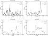 |
Fig. 1 Top left plot: flux time series for the longest observation time (5 days). Top right: flux time series with the largest flux variations. Bottom left: one of the unusual flux time series (gaps and some uncharacteristic flux behaviour). Bottom right: strange flux variations characteristic for the last two of our sessions. The bar in the top-left corner of each subplot represents 1σ flux error for each session. |
2. Observations and analysis
We have carried out a flux density monitoring of PSR B0329+54 during three years using the 32-m Toruń Centre for Astronomy radiotelescope. Observations were performed between July 2002 and June 2005 at the frequency of 4.8 GHz. Twenty epochs of flux density monitoring at 4.8 GHz have been collected (see Table 1). Typical observations lasted about 12–30 h in 3 min scans. During the first two years of our campaign each epoch was at least 24 h; for the third year we observed this pulsar only occasionally, for about 12 h each epoch. In addition, the first observing session lasted a full 5 days, and some other were almost 2 day long.
The total intensity signal was obtained using the Penn State Pulsar Machine II (PSPM II). This pulsar back-end is basically a 64 channel fast radio-spectrometer, which was designed to conduct timing observations and search for pulsars (see Konacki et al. 1999). The PSPM II is currently equipped with additional system that allows mean flux calibration. A dual-circular polarization signal from the total bandwidth of 192 MHz is fed into the backend, and then split into 64 channels (of 3 MHz width each, separately for each polarization). Signals from both polarizations in each channel are then added, and sampled with a rate of 4096 samples per period, thanks to a system that allows dynamical changes of the sampling rate during the observation. This makes data much easier to integrate over time, which in fact is done in real-time. At the same time the noise diode signal is injected once per pulsar period, always on the same phase, which was at least 0.3 different from the actual pulse phase. As a result we have got 64 integrated pulse profiles with a calibration mark for each single observation. Data from all channels were dedispersed and integrated over the whole bandwidth in an off-line procedure.
To obtain flux densities, we carried out regular calibration measurements using the same signal of a noise diode, which was compared to the flux density of known continuum calibrators. Pulsar observations were interrupted regularly for the calibration procedure roughly every 6–8 h (such calibration breaks took about one to one and a half hours), and sometimes there were unforeseen breaks owing to the telescope failures and hardware problems.
2.1. Flux density measurements
Figure 1 shows four of the total 20 flux time-series as observed during our campaign. Subplot (a) represents the flux variation during the longest observing session, i.e. the first epoch in our campaign, that lasted for five days. Evidently, flux variations happen at more than one timescale; the detailed analysis is presented in the next sections. Subplot (b) shows the epoch with the highest measured flux value in our campaign. The maximum averaged flux for a single 3-min integration reaches almost 200 mJy, which means more than 10-times the average value ( ⟨ F ⟩ = 17.4 mJy, see Table 1). This value is also close to the average flux of PSR B0329+54 at 1400 MHz (203 mJy according to ATNF pulsar catalogue). An example of one of the worst quality sessions is shown in subplot (c). There are many gaps in the data taken at that epoch, some are the regular calibration breaks, but others are caused bye the telescope/hardware failures. With all those gaps and some uncharacteristic flux variation it was not possible to conduct a proper analysis for this epoch (confront Table 1 and Sect. 2.4 for detailed explanation). The last subplot (d) shows the flux variations for the penultimate epoch. Again, the flux variations are not typical for our data, the value stays well above the average for a very long time (more than 300 min). This kind of variability makes some kinds of statistical analyses unreliable, i.e. we were not able to find the scintillation timescales because the structure function of the flux time series for this data set does not saturate. At the same time one has to note that this behaviour is quite typical for PSR B0329+54, at least in our data. If one confronts the flux variations from subplot (d) with the longest time series (subplot (a)), one can easily find a matching behaviour – clearly visible between 1000 and 1700 min during the 5-day session. For the epoch shown in subplot (d), which lasted only for 800 min, we were just “unlucky” to catch this kind of variation and not the regular scintillation pattern. The same applies for the last session, with average flux value also exceeding the general average calculated from all sessions (see Table 1).
Because these last two sessions were so untypical for this pulsar, we decided to calculate the general average flux value, and also the average modulation index, with and without them. Both results are shown in Table 1. This table presents the results of the mean flux measurements, averaged over each observing session ⟨ F ⟩ , along with their standard deviations ( ), which also include the contribution from the calibration source uncertainty. We also present the flux modulation indices calculated for individual sessions (see Eq. (1)), these will be discussed in detail in the following sections of this paper.
2.2. Individual session flux density variations
The modulation index m is defined as the ratio of the rms deviation to the mean value of the observed flux densities 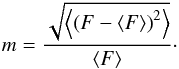 (1)Table 1 presents the values of the measured modulation indices for each individual session. The average values of m in the bottom section of the table, just as the flux density averages (see previous section), are calculated with and without last two sessions. For these sessions the quasi-stable flux behaviour means that the relative strength of the modulation drops and also causes the increase of ⟨ F ⟩ . Both these effects contribute to the decrease of the measured modulation index for the two ultimate sessions.
For the remaining sessions the modulation index varies from 0.71 (November 2002) to 1.32 (August 2002), with an average value of m = 0.96 ± 0.04, which means that the observed flux density of the source is undergoing significant variations. One has to ask a question: what contributes to the observed flux modulation?
We expected that at the frequency of 4.8 GHz PSR B0329+54 will be still in strong scintillation regime, which means that its signal will be undergoing diffractive as well as refractive scintillations. This came from the observational experience with this pulsar and strong flux variability observed at 5 GHz, when we observed it for the purpose of estimating its spectrum (Maron et al. 2000). The theory (see Lorimer & Kramer 2005, for summary) predicts that at 4.8 GHz a pulsar with DM = 26.8 pc cm-3 should be close to its transition frequency, but on the strong scintillation side as well.
For the DISS the intrinsic modulation index should be close to unity. In usual, low-frequency observations, where the decorrelation bandwidth ΔνDISS is significantly less than the observing bandwidth, the number of observed scintles within the bandwidth, at any given time, will be large. That would lead to the decrease of the modulation of the average pulsar flux (integrated over the whole bandwidth), as at any given time, one would see multiple scintles, possibly in different stages of development.
Our observing bandwidth of 192 MHz is at least four times more narrow than the expected ΔνDISS (see Table 3). It means that at any given time we are usually able to see only a fraction of a single scintle. Following Cordes & Lazio (1991), we estimated our number of scintles in both frequency and time, and calculations yielded Nf to be very close to unity (as expected) and Nt ≃ 4.6. The latter leads to the expected DISS modulation index of 0.466, much lower than the observed values. However, after including the contribution from RISS (mRISS = 0.56; the value found via structure function analysis, see next sections of the paper), and using the total intensity variance formula (Rickett 1990), we obtained the final expected value of mtot = 0.889. This value is still somewhat lower than the observed modulation indices, but not by a huge margin.
2.3. Average flux density variations
Because every individual session was at least several hours long, we believe that diffractive scintillations (which happen at the timescale of ca. 40 min, see Sect. 2.4) should not affect our average flux measurements. On the other hand, refractive timescales, which are significantly longer, may have affected our results.
Figure 2 shows the results of the average flux density measurement versus the observing epoch. Clearly (conf. Table 1) there is significant variation in the average values. Using these data, we calculated the modulation index of the average flux density measurements, which yielded the value of m = 0.57. Assuming that the pulsar itself is not varying in intensity, this modulation could be caused by only the refractive scintillations, which happen at significantly long timescales, close to the length of a single observing session.
To take that into account, we calculated the errors of average flux measurements following Kaspi & Stinebring (1992, KS92) as 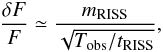 (2)where Tobs is the length of a given observing session, and tRISS is the RISS timescale. To calculate the error values shown in Fig. 2 we used the value of tRISS obtained via the structure function analysis (305 min, see Sect. 2.4).
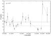 |
Fig. 2 Flux density for each epoch of flux density monitoring at 4.8 GHz. The error of the mean flux density was calculated from σF/F ≈ mRISS/(tobs/tRISS)0.5 (KS92). The top horizontal line represents the arithmetic average flux, the lower line corresponds to the weighted average flux. |
Using those error estimates, we were able to calculate the weighted average flux density ( ) for our entire observing session, which is ⟨Ftot⟩ = 11.69 mJy. This value is shown in Fig. 2 as a dashed-dotted horizontal line, along with the simple arithmetic average from Table 1 (dashed line).
As we mentioned above, the average flux values and their respective uncertainties for the last two sessions in our project differ significantly from the remaining observations. However, a proper calculation of the error estimates improves the picture. For relatively short sessions, which we had towards the end of the project, RISS can play a huge role, but the duration of the session is included in the uncertainty estimates, which makes them more reliable than the formal errors cited in Table 1. The weighted average is therefore much lower than the arithmetic average.
At this point one has to note that the estimation of the flux density of pulsars at high observational frequencies will always be affected by strong scintillations (except for some very low DM cases) and one has to take it into account when trying to measure the flux of these, for example for the purpose of acquiring pulsar spectra.
2.4. Structure function analysis: timescales
To estimate the scintillation timescales, we used the structure function analysis of the flux density variations. For uniformly sampled data the first order of the normalized structure function of the flux density is (Simonetti et al. 1985) ![\begin{equation} D(j)=\frac{1}{\left<F \right>^2 N(j)} \sum w(i)w(i+j)[F(i) - F(i+j)]^2, \end{equation}](/articles/aa/full_html/2011/10/aa16850-11/aa16850-11-eq38.png) (3)where i is the data index, j is the offset that corresponds to a time lag in the data for which the value of the structure function is calculated. w(i) is the weighting factor (which is equal to 1 where the flux density exist for jth points and 0 otherwise), and N(j) = ∑ w(i)w(i + j) is the number of pairs of values found in the data that were found to have the offset equal to j (i.e. time lag equal to τ).
(3)where i is the data index, j is the offset that corresponds to a time lag in the data for which the value of the structure function is calculated. w(i) is the weighting factor (which is equal to 1 where the flux density exist for jth points and 0 otherwise), and N(j) = ∑ w(i)w(i + j) is the number of pairs of values found in the data that were found to have the offset equal to j (i.e. time lag equal to τ).
The values of the structure function need to be corrected to remove white noise contribution. This was made by subtracting the value of the structure function at the unit lag from all the structure function values. If a quasi-periodic signal is present in the data the structure function will show a plateau at the value of Dsat. The timescale of the observed variability is the lag corresponding to half the saturation value of the structure function after white noise correction: tISS = τ(Dsat/2) (KS92).
The error of the timescale can be estimated by finding the time lags that correspond to the values of the structure function of  . The uncertainty of the saturation value of the structure function δDsat is best estimated as δDsat/Dsat ≈ (2tISS/Tobs)1/2, where Tobs is the total duration of the observation, in our case the length of an individual observing session.
Since our project consisted of several observing sessions repeated over the course of three years, we decided to calculate the general average structure function as well. This can be made either directly by applying structure function algorithm to the entire set of data, or by adding the values obtained for individual sessions, after de-normalizing them.
The values of the scintillation timescale, modulation index and their uncertainties for the general average structure function can then be calculated in the same manner as for the individual sessions.
Parameters calculated from structure function for flux density series: scintillation timescales and flux modulation indices.
Table 2 shows the results of the structure function analysis applied to our data. This table has less individual session entries than Table 1 because it shows only those sessions for which the structure function saturated. The saturation of the SF was necessary to calculate the cited values of tISS and m and their uncertainties (see the notes for Table 1).
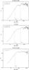 |
Fig. 3 Three structure functions of our data. From top to bottom: the structure function from the 5-day session, general average structure function, and the typical structure function of an individual session (see text for details). |
Figure 3 shows three of the structure functions obtained during the analysis. The top plot shows the SF for the first and longest, 5-day session that was conducted between 2002 July 3–8. This structure function clearly shows two plateaus, which allowed us to obtain the values of two distinctive timescales present in the data. As we mentioned above, at the observing frequency of 4.8 GHz PSR B0329+54 is believed to be close to the transition frequency, i.e. switching from strong to weak scintillation regimes, diffractive and refractive timescales should be relatively close (yielding a low value of the strength of the scattering parameter u). Hence we are convinced that those two plateaus correspond to two scintillation timescales, a shorter diffractive timescale (lower plateau), and a longer refractive timescale.
This is even more convincing for the middle plot of Fig. 3, which shows the general average structure function. Two plateaus were also present for another session, 2002 September 18–19 (ca. 30-h session).
The third and bottom subplot of Fig. 3 shows a typical structure function, obtained during a single, typical 37-h session, where one can see only the regular saturation of the structure function caused by the diffractive scintillations.
The horizontal lines in all those plots show the SF saturation levels, vertical lines – the time lags that correspond to the saturation (the values of the timescales are given in minutes), while the short horizontal dashes crossing them represent the errors in the timescale estimates.
All detailed results are presented in Table 2. The values of tRISS for individual sessions differ from the average SF values. This is understandable because the RISS saturation level is determined with lower precision, because it is limited by the maximum time lag of the SF calculated for the given session, and because especially in the September 2002 we saw only 4–5 RISS cycles. This translates into a large uncertainty of tRISS. While for the September 2002 session the values agree with those obtained from the general average SF within error estimates, for the first and longest July 2002 session they do not. This may be because this session may also suffer from the untypical flux variations that were observed (see Fig. 1 and Sect. 2.1).
Because the general average structure function of our data is the best representative for our results, we’ll be using those values for further calculations: tDISS = 42.7 min, tRISS = 305 min. Given these, we can calculate the strength of the scattering parameter  .
.
Also, since in our observations we were unable to obtain the value of the decorrelation bandwidth BDISS (this value greatly exceeds the total observing bandwidth of PSPM 2, which is 192 MHz) we used the results of our timescale measurements to estimate this value. Using the Stinebring & Condon (1990) formula:  (4)we obtained a value of BDISS = 853 MHz (over 4 times higher than the observing bandwidth).
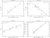 |
Fig. 4 Frequency dependence of diffractive timescales tDISS (top left), refractive timescales tRISS (top right), refractive modulation index mRISS (bottom left), and decorrelation bandwidth BWmRISS (bottom right). Data taken from Bhat et al. (1999) at 327 MHz, Gupta et al. (1994) at 408 MHz, Stinebring et al. (1996) at 610 MHz, Wang et al. (2005) at 1.5 GHz, and this paper at 4.8 GHz. The solid line presents the fit to observed data. |
Estimated and observed parameters.
2.5. Modulation indices from the structure function analysis
As we mentioned in the previous section, the structure function analysis allows us to calculate not only the scintillation timescales, but also their respective scintillation indices. For a normalized and white-noise corrected structure function the value of the scintillation index m = (Dsat/2)1/2, and the fractional error in m is a sum of errors from the fractional errors in Dsat and m (see KS92).
Table 2 shows the results for the individual sessions as well as for the general average SF for the modulation indices of both diffractive and refractive scintillations.
For the diffractive scintillations the average value of mDISS, obtained from the simple arithmetic average of the individual values agrees with the value obtained from general average structure function, which is equal to mDISS = 0.89. This value differs slightly from the modulation index value obtained directly from flux density measurements (0.96, see Table 1), but is very close to the expected value for the observed modulation index (0.889, see Sect. 2.2).
The values of the RISS modulation indices are also presented in Table 2. For individual sessions that allowed for an estimation of mDISS, they differ slightly from the average values, but still agree within the error estimates. This is not a surprise, because it is difficult to determine the saturation level properly, especially for the shorter sessions (for the same reasons the timescales differ, see previous section). On the other hand, the value of mRISS = 0.56 obtained for the general average structure function is very close to the value of the RISS modulation index obtained from the average flux density variation analysis (0.57; see Sect. 2.3 and Fig. 2).
Again, as in the case of the ISS timescales, we will be using the values obtained for the general average structure function as the final result of our analysis: mDISS = 0.89 and mRISS = 0.56.
3. Discussion
The results obtained from the analysis of our observations suggest that we definitely see both refractive and diffractive scintillations affecting the measured pulsar flux density. We were able to calculate both the timescales and modulation indices for these, and also to estimate the expected decorrelation bandwidth.
Our observations were performed at the frequency of 4.8 GHz, for which there is only one observational report to be found in the literature by Malofeev at al. (1996). This was quite a short project, because PSR B0329+54 was only observed for 130 min at this frequency, which given the values of the scintillation timescales we found makes the results unreliable. On the other hand, adding our results to the scintillation parameters estimates obtained by other authors at lower frequencies allows us to study the frequency dependence of these parameters over a much wider range of frequencies.
3.1. Flux density measurements
As we mentioned above, PSR B0329+54 at the observing frequency of 4.8 GHz shows large flux density variations owing to ISS. For some of the individual 3-min integrations the flux measurements yielded values as high as 200 mJy, over 10 times higher than the average value. Those variations happen at a variety of timescales, ranging from minutes to hours, and up to days (cf. Fig. 1a). This clearly shows the dangers of estimating pulsar flux densities at high frequencies (especially for low-DM pulsars) from observations that are based on a limited number of separate integrations, which is often the case when one tries, for example, to ascertain the pulsar spectrum. The diffractive timescale is longer at high frequency, and may be comparable to the actual integration times used – usually of the order of a few tens of minutes when one tries to measure the flux density of some weaker sources – hence, it may strongly affect the outcome. On the other hand, with refractive timescales of the order of a few hours, repeating the observations after a day or a few days, with the hope that the ISS will be averaged-out, may not solve the problem. One has to approach these cases carefully; luckily, for high-DM pulsars this should be less of a problem, because the transition frequency will be much higher and the modulation caused by RISS should be very low, and one has to worry only about diffractive scintillations when performing flux measurements.
In case of our observations of PSR B0329+54 we were able to ascertain the impact of interstellar scintillations on our measurement pretty well. Both our values: 18.4 mJy from the simple arithmetic average and 11.7 mJy from the RISS weighted average agree well with the simple power-law spectra for this source, with spectral index of –2.2 (see Maron et al. 2000, and the authors on-line spectra database at http://astro.ia.uz.zgora.pl/olaf/paper1/index.html).
3.2. Scintillation parameters
Pulsar B0329+54 is one of the strongest radio pulsars known so far, and scintillations of its radiation were analysed at various frequencies by many different authors, especially over the course of last 20 years. Table 3 and Fig. 4 summarize the results we were able to find.
Table 3 shows the list of all scintillation parameters for PSR B0329+54 at different frequencies ranging from 74 MHz to 4.8 GHz. At 4.8 GHz, at which we conducted the observations as well, we only found one measurement of tDISS in Malofeev et al. (1996), which is 21.4 min, almost exactly two times lower than our value from the general average structure function. This discrepancy may arrise because Malofeev et al. (1996) observations were very short: 130 min only, i.e. three diffractive cycles, according to our results. Additionally, one has to note that even during our observations we found that for individual sessions the measured value of tDISS can go as low as 19.0 min (see Table 2). Malofeev et al. (1996) also estimated a lower limit for the diffractive modulation index (mDISS > 0.5).
Figure 4 shows the frequency dependence for both diffractive and refractive scintillation timescales (top right and top left, respectively). Data taken from the literature are represented by full circles (for reference see Table 3), our measurements are the open circles. Evidently, our measurements for both tDISS and tRISS roughly agree with the previous, lower frequency estimates in a sense that they support the theory that the frequency dependence of the scintillation timescales is really governed by a simple power-law. Adding our points to these plots extends the frequency range significantly, which in turn allows for better fit of the power-law to the data. This is especially important for the RISS timescale, because it is very long at lower frequencies and the measurements often suffer because they are either poorly sampled or have only short time spans; i.e. do not cover a sufficiently large number of observed refractive cycles. These result in a large spread of tRISS measurements at lower frequencies.
On the other hand, our measurements were obtained from the continuous observations that usually covered at least 4–5 refractive cycles (in a normal one-day session) and up to over 20 cycles (for the longest 5-day session), which makes them very reliable.
Using the data summarized in Table 3 we performed power-law fits, which yielded  (min) and
  (days).
Similar fits were performed for the RISS modulation index (see bottom left plot in Fig. 4) and the decorrelation bandwidth BDISS, although the latter is not a direct measurement but only an estimate (see Sect. 2.4). Nevertheless, both measurements roughly agree with expectations based on lower frequency data, and adding our points to the pool allowed us to obtain the frequency dependencies as  and
and  .
.
We have to note that for the purpose of two of these fits, namely tRISS and mRISS, we decided to omit the values obtained by Wang et al. (2008), which are represented by triangles in their respective plots. These points stray by much from the rest of the data, and contradict the earlier estimates at the same frequency (1540 MHz) given by Wang et al. (2005). Adding our values to the data pool clearly shows that their earlier results (obtained from a different set of observations) seem to fit better into the general picture. We believe that the 2008 results are flawed; problem may lie in the method that was used for the purpose of that paper. Based on other data, the actual refractive timescale at 1540 MHz should be of the order of 2 days (similar value as that given by their earlier paper, which is 2.5 days). Their observations were conducted almost continuously for 20 days in March 2004, with the flux measurements based on 90-min integrations. At the frequency of 1540 MHz this means that they observed only a few diffractive cycles during their single flux-integration, which may have affected the measurements. The authors calculated mRISS based on that data. However, their structure function for the flux measurements did not saturate. Without the saturation level it is impossible to estimate the timescale from the structure function (see Sect. 2.4), and they decided to obtain the saturation level as Dsat = m2/2 (see Sect. 2.5). Using the value obtained this way, and applying it to the structure function (see their Fig. 5), they inferred the value of the RISS timescale of 8 h, 6 times lower than expected and almost 8 times lower than in their previous paper.
Probably the flaw lies in the underestimation of the RISS modulation index (which clearly shows in our Fig. 4 as well) which resulted in a lowering of the used saturation level. An inspection of the structure function they obtained (see their Fig. 5, Wang et al. 2008) leads to the conclusion that even a slight change of mRISS, and in turn the saturation level Dsat, could lead to timescale even a half an order of magnitude higher than the 8 h they quote, and we think that is exactly what happened. In Wang et al. (2008) defense we may note that we had one session in our data that is coincident with their March 2004 observations, as we performed a 38-h observation between March 15 and 17 of 2004, and our structure function did not saturate as well, which may suggest that the fluctuations of the flux density were untypical during that period.
Knowledge of frequency dependence of both tDISS and tRISS gives us an opportunity to calculate the transition frequency, i.e. the observing frequency at which both timescales would be equal, which means a switch from strong to weak scintillation regimes. Using the empirical formulae provided above (see also Fig. 4) and putting both timescales equal, this yields the transition frequency νc of 10.1 GHz. Below this frequency PSR B0329+54 will be in the strong scintillation regime, above that frequency, the characteristic of the scintillation should change to weak scintillations.
3.3. Estimation of electron density turbulence spectrum
Observations of the interstellar scintillations and especially the frequency dependence of the measured parameters can be used to estimate the properties of the interstellar turbulence. By analogy to the neutral gas theory, the density fluctuations in the ISM can be described by a power-law spectrum as  , where
  is the mean turbulence of electron density along the line of sight, q = 2π/s is the wavenumber associated with the spatial scale of turbulence s, and the spectral index β, which is in range of 3 < β < 5. The well known Kolmogorov theory developed for neutral gas turbulence yields the spectral index of β = 11/3, but it was shown by several authors (see for example Gupta et al. 1993) that there are discrepancies between Kolmogorov theoretical predictions and actual measurements of scintillation parameters for some pulsars. Few models of the interstellar turbulence with different spectral slopes β were developed, yielding different sets of predictions of the frequency dependence of ISS parameters (see Romani et al. 1986; Bhat et al. 1999). Table 4 summarizes these predictions for the three most commonly used spectral slopes of β = 11/3 (Kolmogorov spectrum), 4 and 4.3 for the four scintillation parameters we were able to measure, or derive from our observations of PSR B0329+54. Our estimations of the actual spectral slopes of these parameters, based on all available data (see Sect. 3.2 and Fig. 4) are also in the table.
Apparently none of the currently models for the electron turbulence agrees precisely with our estimations, and the model predictions with β = 4 are the closest to the slopes we obtained from our fits. It has to be noted that in case of three of the four parameters (with the mRISS being the only exception), these discrepancies cannot be attributed to poor quality of frequency slopes fits for these parameters, especially that our measurements, made at the frequency of 4.8 GHz, significantly widened the frequency range, putting strong constraints on the fits.
3.4. Derived scintillation parameters
As we mentioned above, in a strong scintillation regime the flux density variations happen at two distinctive timescales – diffractive and refractive. The apparent variability of the pulsar signal can be understood as the result of the observer crossing the diffraction pattern, which is introduced by the ISM to the pulsar signal wavefront. In a thin screen model, those two timescales correspond to two spatial scales of the diffraction pattern: the diffractive scale sd, and refractive scale sr, which in turn can be bound to the concepts of scattering angle and scattering disk that is commonly used in the scintillation theory (see Rickkett 1990).
Following Gupta et al. (1994), we can find the diffractive scale by the means of estimating the scintillation velocity VISS, which is bound to the diffractive scale as sd = VISStDISS. The scintillation velocity can be derived from the diffractive timescale tDISS and the decorrelation bandwidth BDISS (Cordes 1986; Gupta et al. 1994). Using our values in the formula yields  km s-1.
The observed scintillation velocity should be modulated by the Earth’s orbital motion, but our data proved to be inconclusive in that regard. We only had the diffractive timescale measured for each epoch, and were forced to use the average value of decorrelation bandwith (and/or refractive timescale) in the VISS formula, which led to a wide spread in the VISS versus epoch data, making our fits unreliable. Measurement of the refractive timescale for every epoch would probably solve the problem, as would the direct measurement of the decorrelation bandwidth, but these were impossible owing to the character of the variability of the pulsar flux and the limited observing bandwidth of the backend used.
The average value of VISS = 92.9 km s-1 combined with the measured tDISS = 42.7 min. yielded the diffractive scale sd = 2.38 × 10⁸ m.
The diffractive angle θd can be estimated from (Wang et al. 2005) 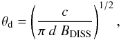 (5)where c is the speed of light. This yields θd = 0.01207 milliarcsec, which translates into the refractive scale sr = 1.91 × 10⁹ m. Combining this with the previously obtained value of diffractive scale sd, we can estimate the Fresnel scale for the observed ISS as rF = (sdsr)1/2 = 6.7 × 10⁸ m.
One has to remember that for observations we were not able to measure the decorrelation bandwidth BDISS directly, and both of the formulae for VISS and θd are based on this value.
The value of the strength of the scattering parameter inferred from the spatial scales sr and sd is u = 2.84, which is slightly different from the value derived from the scintillation timescales (u = 2.67, see Sect. 2.4). The discrepancy is small, however, and given the fact that the application of the ISS theory to the observations always involves lots of approximations and assumptions, our values of sr,sd and rF we got are as reliable as possible.
4. Summary and conclusions
We presented the results of our three-year observing project of PSR B0329+54 at the frequency of 4.8 GHz, using the 32-m Toruń Centre for Astronomy radiotelescope and the Penn State Pulsar Machine II as a backend. The project was very unique, because it consisted of twenty separate observing sessions, each of them involving several hours (up to 5 days; more than 24 h on average) of continuous observations of the flux density of the pulsar, with 3-min time resolution. The total observing time ammounted to 35 thousand minutes, or 24 days, making it probably one of the longest observing programmes that involved long-term continuous observations of flux density and scintillation parameters that was performed using a single observing setup and uniformly analysed from raw data to the final results.
4.1. Scintillation parameters at 4.8 GHz
The analysis of the data allowed us to conclude that flux density variations are governed by two distinctive timescales, which we identify as the diffractive and refractive scintillation timescales. The fact that the observing frequency of 4.8 GHz is relatively close to the transition frequency for this pulsar makes those timescales differ only by a factor of ~7. The character of our observations allowed us to detect them both at the same time, by means of the structure function analysis, using the same set of data – twice for individual sessions and additionally by constructing general average structure function. To our knowledge this is the first case of pulsar ISS observations where both scintillation timescales were measured from a single data set using exactly the same method.
The measured values of the diffractive timescale  min and refractive timescale
  min allowed us to estimate the decorrelation bandwidth (unobtainable via direct measurements, because it exceeds the observing bandwidth of the backend used) as BDISS = 853 MHz. Also, we were able to estimate the strength of scattering parameter, which can be expressed as square-root of the timescale ratio, as u = 2.67.
We were also able to estimate the amount of modulation that both types of scintillation contribute to the flux variability, and did that by the means of the modulation indices. Especially important is the estimation of the modulation due to refractive scintillations, for which the modulation index is relatively strong: mRISS = 0.56. This agrees with the fact that during some of our observing sessions we noticed very drastic flux density variations, with the flux from single 3-min integration reaching the values of 200 mJy, exceeding the average value by a factor of ~20.
This shows how important it is to take ISS into account when measuring pulsar flux densities at high frequencies, especially for low-DM pulsars. For these objects the frequency of the switch from strong to weak scintillation regimes (i.e. the transition frequency) should be relatively low, and all theories predict the increase of refractive modulation index towards that frequency (for summary see Lorimer & Kramer 2005; also Romani et al. 1986). In these cases, when the ISS timescales are of the order of tens to a few hundred minutes, typical flux density observations (which usually involve continuous integration of the length of 10 min to an hour) of a single measurement may be heavily affected by both types of scintillations. This in turn may cause problems when trying to construct the pulsar spectra, leading to artificial breaks or turn-ups observed in the spectrum - as was pointed out in a few cases by Maron et al. (2000). The only way around the problem is to repeat the measurement several times to average-out the influence of ISS. Luckily, this should be less of a problem for pulsars with higher dispersion measures because the transition frequency for such objects should be well outside the usual observing frequencies, meaning that at least the refractive scintillations should not affect the measurement by much. Still, the diffractive scintillations would present a problem if their timescale would be similar to the integration lengths used, so one should approach every case carefully and individually.
Our measurements of the scintillation timescales allowed us also to estimate some of the parameters commonly used to describe the theory of interstellar scintillation. We were able to estimate the Fresnel scale rF as 6.7 × 10⁸ m, which at the frequency of 4.8 GHz corresponds to a refractive scale of sr = 1.9 × 10⁹ m, and the diffractive timescale of sd = 2.4 × 10⁸ m.
We were also able to estimate the scintillation velocity of VISS = 92.9 km s-1, and we hope that our value will help to solve the problem with the discrepancies that can be found in the literature. It agrees well with Wang et al. (2005) as they obtained 97 km s-1, on the other hand KS92 report VISS = 68 km s-1, whereas Gupta (1995) 170 km s-1 or 126 km s-1, depending on the model. One has to remember that those discrepancies may arise because while the the formula is uniform (with the possible exception of the scaling factor Av), the ways used to obtain the parameters were usually different.
4.2. General picture
Adding our results to the estimations of the scintillation parameters at lower frequencies that can be found in the literature allowed us to study the dependence of these parameters on the observing frequency. That our observations were conducted at the frequency of 4.8 GHz proved to be very useful because it significantly widened the frequency range for which the values of ISS parameters are known. Previous attempts at this analysis were limited to the frequency of ~1.5 GHz, adding our measurement expanded that range three-fold, which means an extension of ca. 50% when talking about the log-scale in frequency. This proved to be especially helpfull for the RISS parameters. At low frequencies the RISS timescale is very long and the modulation very weak, which brings a relatively large scatter to the low-frequency parameter estimates, making any attempts to fit a power-law type dependency questionable. The addition of our results, which we believe to be very reliable (because they come from a long-term monitoring programme), improves the general picture greatly (see Fig. 4), making any fits to the data much more constrained.
We performed the fits of the power-laws governing the frequency dependence of the scintillation parameters, and they yielded us the respective spectral indices, which can be expressed as: tDISS ~ f 1.01, tRISS ~ f − 1.76, mRISS ~ f 0.32 and BDISS ~ f 3.68. These values significantly differ from those predicted by using Kolmogorov neutral gas theory to the ISM spatial electron density spectrum (β = 11/3, see Table 4). Indeed our measurements do not agree with any of the models describing the electron density spectrum that are commonly used, with the model using β = 4 being the closest to the obtained spectral indices. This would indicate that the real spatial electron density spectrum is steeper than the Kolmogorov spectrum. Unfortunately, the character of our data did not allow for the estimation of the β index by the means used by a few other authors (see for example Wang et al. 2005) because they usually involve measurements performed in the dynamic spectra.
Using the above mentioned formulae we were able to estimate the transition frequency for PSR B0329+54, i.e. the frequency at which the transition from strong to weak scintillation mode should appear, which is νc = 10.1 GHz. This clearly contradicts the earlier statement of Malofeev et al. (1996), which estimated the transition frequency to be around 3 GHz. This value is also higher than the transition frequency one can infer from Lorimer & Kramer (2005) – namely from their Fig. 4.3, which suggests that for a pulsar with DM = 27 pc/cm3νc should be close to 4 GHz.
It would be extremely interesting, but on the other hand very hard, to perform an observing project similar to ours at a frequency close to this transition frequency. First – the pulsar would be much weaker, thus requiring longer integration times. On the strong-scintillation-regime side of the transition frequency, the two ISS timescales would be extremely similar (100 min), which means that the distinction between them would be very hard to make, and would probably require very long sets of continuous observations. Because there are only a handful of telescopes that could perform these observations (i.e. have the required receiver equipment), this may be impossible to accomplish.
Nevertheless, any type of scintillation or flux density variation observations, performed at the frequency close to the transition frequency, may be very helpful to our understanding of the scintillation phenomenon in general, and the switch from strong- to weak-scintillation in particular. This is also true for other pulsars, especially those with lower dispersion measures, because the expected transition frequencies for them would be even lower than the 10 GHz for PSR B0329+54.
Acknowledgments
We are grateful to G. Hrynek for his help with our observations and the calibration procedure. J.K., K.K. and W.L. acknowledge the support of the Polish State Committe for scientific research under Grant N N203 391934.
References
- Bhat, N. D. R., Rao, A. P., & Gupta, Y. 1999, ApJS, 121, 483 [NASA ADS] [CrossRef] [Google Scholar]
- Cordes, J. M. 1986, ApJ, 311, 183 [NASA ADS] [CrossRef] [Google Scholar]
- Cordes, J. M., & Lazio, T. J. 1991, ApJ, 376, 123 [NASA ADS] [CrossRef] [Google Scholar]
- Esamdin, A., Zhou, A. Z., & Wu, X. J. 2004, A&A, 425, 949 [NASA ADS] [CrossRef] [EDP Sciences] [Google Scholar]
- Gupta, Y. 1995, ApJ, 451, 717 [NASA ADS] [CrossRef] [Google Scholar]
- Gupta, Y., Rickett, B. J., & Coles, W. A. 1993, ApJ, 403, 183 [NASA ADS] [CrossRef] [EDP Sciences] [Google Scholar]
- Gupta, Y., Rickett, B. J., & Lyne, A. G. 1994, MNRAS, 269, 1035 [NASA ADS] [CrossRef] [Google Scholar]
- Hewish, A., Bell, S. J., Pilkington, J. D. H., Scott, P. F., & Collins, R. A. 1968, Nature, 217, 709 [NASA ADS] [CrossRef] [Google Scholar]
- Kaspi, V. M., & Stinebring, D. R. 1992, ApJ, 392, 530 (KS92) [NASA ADS] [CrossRef] [Google Scholar]
- Konacki, M., Lewandowski, W., Wolszczan, A., Doroshenko, O., & Kramer, M. 1999, ApJ, 519, L81 [NASA ADS] [CrossRef] [Google Scholar]
- Kramer, M., Xilouris, K. M., & Rickett, B. 1997, A&A, 321, 513 [NASA ADS] [Google Scholar]
- Lorimer, D. R., & Kramer, M. 2005, Handbook of Pulsar Astronomy (Cambridge University Press) [Google Scholar]
- Malofeev, V. M., Shishov, V. I., Sieber, W., et al. 1996, A&A, 308, 180 [NASA ADS] [Google Scholar]
- Maron, O., Kijak, J., Kramer, M., & Wielebinski, R. 2000, A&AS, 147, 195 [NASA ADS] [CrossRef] [EDP Sciences] [Google Scholar]
- Rickett, B. J. 1990, ARA&A, 28, 561 [NASA ADS] [CrossRef] [Google Scholar]
- Rickett, B. J., Coles, W. A., & Bourgois, G. 1984, A&A, 134, 390 [NASA ADS] [Google Scholar]
- Romani, R. W., Narayan, R., & Blandford, R. 1986, MNRAS, 220, 19 [NASA ADS] [Google Scholar]
- Shishov, V. I., Smirnova, T. V., Sieber, W., et al. 2003, A&A, 404, 557 [NASA ADS] [CrossRef] [EDP Sciences] [Google Scholar]
- Sieber, W. 1982, A&A, 113, 311 [NASA ADS] [Google Scholar]
- Simonetti, J. H., Cordes, J. M., & Heeschen, D. S. 1985, ApJ, 296, 46 [NASA ADS] [CrossRef] [Google Scholar]
- Stinebring, D. R., & Condon, J. J. 1990, ApJ, 352, 207 [NASA ADS] [CrossRef] [Google Scholar]
- Stinebring, D. R., Faison, M. D., & McKinnon, M. M. 1996, ApJ, 460, 469 [NASA ADS] [CrossRef] [Google Scholar]
- Stinebring, D. R., Smirnova, T. V., Hankins, T. H., et al. 2000, ApJ, 539, 300 [NASA ADS] [CrossRef] [Google Scholar]
- Wang, N., Nanchester, R. N., Johnston, S., et al. 2005, MNRAS, 358, 270 [NASA ADS] [CrossRef] [Google Scholar]
- Wang, N., Yan, Z., Manchester, R. N., & Wang, X. H. 2008, MNRAS, 385, 1393 [NASA ADS] [CrossRef] [Google Scholar]
All Tables
Parameters calculated from structure function for flux density series: scintillation timescales and flux modulation indices.
All Figures
|
Fig. 1 Top left plot: flux time series for the longest observation time (5 days). Top right: flux time series with the largest flux variations. Bottom left: one of the unusual flux time series (gaps and some uncharacteristic flux behaviour). Bottom right: strange flux variations characteristic for the last two of our sessions. The bar in the top-left corner of each subplot represents 1σ flux error for each session. |
| In the text | |
|
Fig. 2 Flux density for each epoch of flux density monitoring at 4.8 GHz. The error of the mean flux density was calculated from σF/F ≈ mRISS/(tobs/tRISS)0.5 (KS92). The top horizontal line represents the arithmetic average flux, the lower line corresponds to the weighted average flux. |
| In the text | |
|
Fig. 3 Three structure functions of our data. From top to bottom: the structure function from the 5-day session, general average structure function, and the typical structure function of an individual session (see text for details). |
| In the text | |
|
Fig. 4 Frequency dependence of diffractive timescales tDISS (top left), refractive timescales tRISS (top right), refractive modulation index mRISS (bottom left), and decorrelation bandwidth BWmRISS (bottom right). Data taken from Bhat et al. (1999) at 327 MHz, Gupta et al. (1994) at 408 MHz, Stinebring et al. (1996) at 610 MHz, Wang et al. (2005) at 1.5 GHz, and this paper at 4.8 GHz. The solid line presents the fit to observed data. |
| In the text | |
Current usage metrics show cumulative count of Article Views (full-text article views including HTML views, PDF and ePub downloads, according to the available data) and Abstracts Views on Vision4Press platform.
Data correspond to usage on the plateform after 2015. The current usage metrics is available 48-96 hours after online publication and is updated daily on week days.
Initial download of the metrics may take a while.