| Issue |
A&A
Volume 534, October 2011
|
|
|---|---|---|
| Article Number | A127 | |
| Number of page(s) | 13 | |
| Section | Interstellar and circumstellar matter | |
| DOI | https://doi.org/10.1051/0004-6361/201015564 | |
| Published online | 19 October 2011 | |
The mid-infrared extinction in molecular clouds
Case study of B 335⋆
Stockholm Observatory, Stockholm University, Astronomy Department AlbaNova Research Center, 106 91 Stockholm, Sweden
e-mail: This email address is being protected from spambots. You need JavaScript enabled to view it.
Received: 11 August 2010
Accepted: 2 August 2011
Abstract
Aims. The purpose of the present investigation is to probe the dust properties inside a molecular cloud, in particular how particle growth and the presence of ice coatings may change the overall shape of the extinction curve.
Methods. Field stars behind a molecular cloud can be used to probe the cloud extinction for both the reddening and the absorption features. By combining multi-colour photometry and IR spectroscopy the spectral class of the star can be determined as can the extinction curve, including the vibrational bands of ices and silicates.
Results. Based on observations of field stars behind the dark globule B 335, we determine the reddening curve from 0.35 to 24 μm. The water ice band at 3.1 μm is weaker (τ(3.1) = 0.4) than expected from the cloud extinction (AV ≈ 10 for the sightline to the most obscured star). On the other hand, the CO ice band at 4.7 μm is strong (τ(4.67) = 0.7) and indicates that the mass column density of frozen CO is about the same as that of water ice. We fit the observations to model calculations and find that the thin ice coatings on the silicate and carbon grains (assumed to be spherical) lower the optical extinction by a few percent. We show that the reddening curves for the two background stars, for which the silicate band has been measured, can be accurately modelled from the UV to 24 μm. These models only include graphite and silicate grains (plus thin ice mantles for the most obscured star), so there is no need for any additional major grain component to explain the slow decline of the reddening curve beyond the K band. As expected, the dust model for the dense part of the cloud has more large grains than for the outer regions. We propose that the well established shallow reddening curve beyond the K band has two different explanations: larger graphite grains in dense regions and relatively small grains in the diffuse ISM, giving rise to substantially less extinction beyond the K band than previously thought.
Conclusions. For the sight line towards the most obscured star, we derive the relation AKs = 0.97·E(J − KKs), and assuming that all silicon is bound in silicates, N(2 H2+H) ≈ 1.5 × 10²¹·AV ≈ 9 × 10²¹·AKs. For the rim of the cloud we get AKs = 0.51·E(J − Ks), which is close to recent determinations for the diffuse ISM. The corresponding gas column density is N(2 H2+H) ≈ 2.3 × 10²¹·AV ≈ 3 × 10²²·AKs.
Key words: ISM: molecules / ISM: clouds / dust, extinction / scattering / opacity
Based on observations collected at the European Southern Observatory, Chile (ESO programs 073.C-0436(A), 077.C-0524(A)) and on observations made with the Nordic Optical Telescope (NOT), operated on the island of La Palma jointly by Denmark, Finland, Iceland, Norway, and Sweden, in the Spanish Observatorio del Roque de los Muchachos of the Instituto de Astrofisica de Canarias.
© ESO, 2011
1. Introduction
Interstellar reddening is caused by small dust particles, but the detailed optical and chemical properties of these particles remain largely unknown, in particular for molecular clouds. With the exception of the 220 nm extinction peak (probably caused by small graphite grains), the UV, optical, and near-IR spectral regions offer little information about the dust particles, except that they must be small compared to the wavelength (even in the UV). In the mid-IR, however, strong absorption bands show up, the most universal of these being the broad band centred at 9.7 μm due to silicates. Another widespread component in the diffuse ISM (interstellar medium), PAHs (polycyclic aromatic hydrocarbons) are seen in the mid-IR as emission (due to luminescence). In addition, the far-IR thermal emission from the interstellar dust grains gives further constraints on their size distribution, and to some extent, their composition.
Combining all this information, Draine (2003b) has constructed a dust model that describes the observed properties for the diffuse ISM. It basically consists of silicate and carbon grains. For molecular clouds, the lower temperature, the higher density and a diluted UV radiation field allow ices to form and/or condense on the grains. In addition, the grains coagulate and the size distribution is changed towards larger grains. These processes alter the optical properties of the grains. The most obvious difference compared to the diffuse ISM is the absorption features from ices. The ISO instruments provided extensive spectroscopic evidence of various ice absorption features, including H2O, CO, CO2, CH4, CH3OH and NH3 (Gibb et al. 2004). In most cases, these absorption features have been observed towards luminous, deeply embedded protostars, and it is hard to separate the circumstellar matter (influenced by dynamical and radiation processes involved in the formation of the star) from the unprocessed cloud component. In addition, the intrinsic SED (spectral energy distribution) of an embedded young star is not in general well known, which means that it is difficult to accurately separate interstellar reddening from intrinsic IR excess. For these reasons, field stars behind a molecular cloud are better probes in investigations of the (more or less) undisturbed cloud. The problem is to find background stars that are heavily obscured to probe the dense regions and still bright enough for IR spectroscopy. In spite of these difficulties, there are some investigations of ice features using background stars: Elias 16 by Gibb et al. (2004) and Spitzer ice-data from three sources behind Taurus and CK2 in Serpens by Knez et al. (2005). More recently, Boogert et al. (2011) has combined ground-based and Spitzer spectroscopy data to analyse the ice and silicate features in quiescent clouds by observing background field stars.
Apart from the absorption bands, the continuous extinction in the mid-IR for molecular clouds has been the subject of several recent investigations (e.g. Flaherty et al. 2007; Román-Zúñiga et al. 2007; Chapman et al. 2009; Boogert et al. 2011). However, it is important to note that what is actually determined is the reddening curve, and to establish the extinction curve, an assumption is made on the extinction ratio for two wavelengths, e.g. AH/AK = 1.55, which goes back to the frequently cited paper by Rieke & Lebofsky (1985). Their paper combined earlier investigations with mid-IR observations of distant field stars of unknown intrinsic colours. Obviously the data available for their analysis was very limited compared to those in recent investigations, based on large surveys both from ground and space. The reddening curve is relatively straight forward to determine, either by statistical methods (slopes in colour/colour diagrams) or by classifying selected background stars and compare the observed colour to the intrinsic. By observing stars all the way to Spitzer/MIPS 24 μm one would expect that the extinction is so close to zero at this wavelength, that it for all practical purposes does not matter if it is assumed to be exactly zero. However, the observations show that the reddening curve levels off in the mid-IR, which is not expected from current dust models, and for this reason the extrapolation to zero wave number remains uncertain.
In our recent paper (Olofsson & Olofsson 2010, hereafter called Paper II) we confirmed that the reddening curve for molecular clouds in the wavelength range 0.35–2.2 μm can be characterized in a functional form described by (Cardelli et al. 1989, henceforth CCM) with only one parameter, RV = AV/EB − V. It was, however, clear that the CCM function did not adequately describe the reddening curve beyond the K band, and in the present paper we extend the investigation into the mid-IR spectral region. For our case study we have compiled our own and archive data for a few stars behind the B 335 globule including photometry and spectroscopy from the optical region to 24 μm. Our main purpose is to characterize the mid-IR extinction. In addition we explore whether both the reddening curve, from UV to 24 μm, and the absorption features can be explained in a single model.
Observations and data.
2. Observations and reductions
The present investigation is based on observations of a few background stars behind the B 335 dark globule (RA(2000) = [19 37 00], Dec(2000) = [7 34 10]) in both the optical and the near-IR. Their positions are marked in Fig. 1. Table 2 shows the observations available in our investigation.
Summary of the background stars and available measurements.
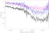 |
Fig. 1 A U band image of the B335 globule. The centre YSO and its outflow region as well as the background stars are marked. The circle represents the position of the 13CO and the C18O measurement closest to the background star #947 in Harjunpää et al. (2004) and the size of the circle represents the 45′′ beam width. |
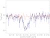 |
Fig. 2 The optical and near-IR extinctions towards the background stars #947 and #90. The extinction for #90 and #947 are well represented by the fitted CCM-extinction with RV = 4.9 (dashed). |
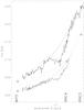 |
Fig. 3 The optical spectrum of the most obscured star (#947) is well represented by a stellar model (from Hauschildt et al. 1999) with Teff 3050 K. The stellar model (red curve) has been modified by a weighting function ∝ λ-1 to account for the interstellar reddening. |
-
Imaging and spectroscopy using the NTT/EMMI at ESO, La Silla (077.C-0524(A) during four nights 2006-06-27–29. These observations and reductions are described in a previous article, (Olofsson & Olofsson 2009, Paper I).
Spectroscopy of the background star (# 947) in the water ice band at 2.7 < λ < 3.8 μm and the CO-ice band at 4.0 < λ < 4.5 μm using VLT-ISAAC at ESO, Paranal during two nights, 2004-04-12–13. A standard star HR7519 is observed before and after each observation of the program star. The 2D-spectra are first corrected for bias and flat-field and the 1D-spectra are extracted with the IRAF program pipeline “APALL”. The program and standard spectra are then divided by respective stellar atmospheric models. These are then divided to correct for telluric atmospheric extinction.
-
Imaging at 3.79 μm using SIRCA (Stockholm Observatory IR CAmera) mounted on the 2.5m Nordic telescope on La Palma.
3. Results
3.1. The intrinsic colours of the background stars
In Paper II we confirmed that the molecular cloud reddening in the optical and the near-IR spectral region is well characterized by a functional form defined by CCM with only one parameter, RV = AV/EB − V. This also allows us to use the multi-band photometry to both determine the RV value and the spectral class for an obscured star as well as the reddening towards it. For the two most obscured stars in the present study, #947 and #90, we get the same RV value, RV = 4.9 (Fig. 2), and their spectral classes are M6III and A0V respectively. The spectral class of the most obscured star in our sample, #947, is of particular importance as it is the only star for which we have water and CO ice data and the temperature determined by the multiband photometry is confirmed both by the optical spectrum (Fig. 3) and the L window spectrum (Fig. 4). The spectral classes of the other stars are also confirmed by optical spectra. This means that we can characterize the intrinsic SEDs (spectral energy distributions) of the stars, and for that purpose we use model atmospheres from Hauschildt et al. (1999).
3.2. The H2O and CO ice bands
By dividing the ISAAC spectra of star #947 (corrected for telluric absorption and relative flux calibrated) with a model atmosphere corresponding to the spectral class of the star (Teff = 3050 K and log g = 0) we determine the absorption of the H2O and CO ice bands (see Figs. 4 and 5 respectively). The peak position of the water ice band is at 3280 cm-1 (=3.05 μm) with an FWHM of 350 cm-1. We note that there is no clear extension shortward of 3000 cm-1 (longward of 3.33 μm). Such an extension is often observed and explained as due to methanol ice (Gibb et al. 2004). The CO absorption peaks at 2140 cm-1 (=4.67 μm), which differs from that of pure CO ice (~2142 cm-1, Elsila et al. 1997), but agrees with observations of other regions (Pontoppidan et al. 2003). There is, however, no indication of wing components, although our S/N ratio does not allow any firm statement on this point.
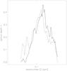 |
Fig. 4 The ISAAC spectrum in the L band of star #947 (blue curve) and the stellar atmospheric model (red curve) are divided to get the water ice band (black curve). |
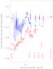 |
Fig. 5 The ISAAC spectrum in the M band of star #947 (blue curve) and the corresponding stellar atmospheric model (red curve) are divided to get the CO ice band (black curve). |
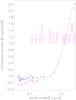 |
Fig. 6 Spectra for sight lines towards stars #2 (lower) and #947 (upper curve) as observed by Spitzer-IRS (#2: 7 < λ < 14 μm) and ISOCAM-CVF (#947: 5 < λ < 16 μm) and photometry from Spitzer-IRAC and Spitzer-MIPS (+ signs). |
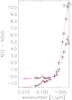 |
Fig. 7 The optical depth of the silicate band τsilicate towards star #2 (dashed line) and #947 (full line) as determined from Spitzer-IRS and ISOCAM-CVF observations, respectively. Although the S/N of the observations does not allows for an interpretation of the details, we note that for star #947 the band peaks at ≈ 0.109 μm-1 corresponding to 9.2 μm. |
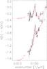 |
Fig. 8 The “reddening” curve in the mid-IR, “normalized excess” = E(λ − Ks)/E(I − Ks) vs. wave number, for six stars behind the B 335 globule. The normalized excess derived from the Spitzer/ISOCAM spectra of two of the stars, #2 and # 947, are included with the same normalization. |
3.3. The silicate absorption band
The B 335 globule was observed with the ISOCAM/CVF and the background M giant (#947) is the only star visible in the field. The LW part of the scan consists of two spectral scans (back and forth) and we have adopted the average of the two. The wavelength coverage is 5 < λ < 16 μm, and except for the longest wavelengths, the S/N is good, see Fig. 6.
Two of the background stars (#2 and #947) have also been observed by Spitzer/IRS in one partial band each, Fig. 6. The Spitzer/IRS and the ISOCAM/CVF spectra of star #947 have been combined to one spectrum. We note that the band peaks at 0.109 μm-1 (=9.2 μm) with an FWHM of ~380 μm. The silicate feature peak is thus found at a shorter wavelengths than e.g. described by Draine & Lee (1984) and Gibb et al. (2004), while the FWHM-widths agree with those found for star forming regions by Gibb et al. (2004). In a recent investigation, Chiar et al. (2011), who investigate absorption bands in the quiescent cloud IC 5146, also show that the silicate band is slightly shifted towards a shorter wavelength. It is also interesting to note that even though #947 is much more obscured than #2, the silicate bands have approximately the same strength. This agrees with the results of Chiar et al. (2011).
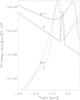 |
Fig. 9 The normalized excess, (E(λ − Ks)/E(I − Ks), in the mid-IR for the weighted average of the five stars at the rim of the B 335 globule (blue) and the most obscured star (red). The green curve represents the Draine (2003a)RV = 5.5 curve. |
3.4. The CO2 band at 15.2 μm
There is an indication in the CVF spectrum of the CO2 band at 15.2 μm but it is not confirmed in the IRS spectrum, which has a higher S/N ratio. We can therefore only give an upper limit τCO2 < 0.15, corresponding to a CO2-column density NCO2 < 3 × 10¹⁷ [cm-2].
3.5. The reddening curve in the mid infrared
For each star in our sample we compare the observed colour indices to that calculated without interstellar reddening. We refer the colour excess to the Ks band
 and normalize by dividing with E(I − Ks). The result is shown in Fig. 8, where we also include the Spitzer spectra. The general impression is that there is not much reddening beyond the Ks band, but in view of the uncertainties involved, both related to the observations and the model atmospheres, we cannot claim that the scatter in the diagram reflects real qualitative variations of the extinction in the intervening cloud. Even though we cannot either exclude such variations, it is in our view meaningful to calculate an error-weighted average for the “rim” stars compared to that of the most obscured stars. The result is shown in Fig. 9 and we find that the extinction is only going down marginally between the Ks band and the silicate band. There is an apparent difference between the extinction in the “rim” region compared to the deeper part of the globule (represented by the direction towards star #947). In view of the uncertainties involved, it is not quite clear that this difference is real, but in the following we assume that it in fact is real and model the two cases separately.
4. Interpretation
4.1. Extinction and grain properties
4.1.1. Grain size distribution
Mathis et al. (1977, henceforth MRN) constructed grain models for the ISM extinction with two simple grain size distributions dN(a)/da for silicates and graphite respectively, both with dN(a)/da ∝ a-3.5 (with a as the grain radius) and 0.001 < a < 0.25 μm. Several attempts to find the grain size distribution of the ISM from the measured extinction have been done. Weingartner & Draine (2001) have elaborated on this and suggested size distributions for graphite and silicate grains based on more than ten parameters and explaining a large wavelength range of the ISM-extinction. We followed their approach to analyze the B335 extinction curve in the optical and near-IR wavelength range (Olofsson & Olofsson 2010).
The same approach in the wavelengths beyond 2 μm for a molecular cloud does not seem to be that successful. We have therefore taken a somewhat simpler approach assuming a modified MRN grain size distribution still with spherical graphite and silicate grains and still using the optical refractive indices as proposed by Draine & Lee (1984) and Draine (2003c) (in tabulated format found at http://www.astro.princeton.edu/~draine/dust/dust.diel.html). We also increased the grain size range to 0.001 < a < 5 μm. The distributions are assumed to follow a power law grain size distribution dN/da (with the spherical grain radius a) for each substance (graphites and silicates): 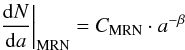 without any restrictions to the parameters. We have furthermore introduced an accumulation of grains with sizes around one grain-size by adding a Gaussian grain distribution to each of the graphite and the silicate MRN-distributions.
 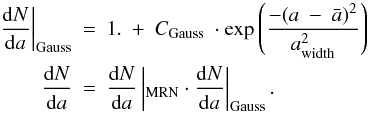 We use a χ2 optimisation scheme to calculate the parameter sets
 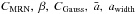 (for graphites and silicates respectively). We find that the two different extinction curves determined above actually can be accurately modelled by this kind of grain size distribution (Figs. 10 and 11). Thus, there is no need to include any other major dust component than silicate and graphite grains. The corresponding size distribution of the grains are shown in Fig. 12. Even though we cannot draw too far-reaching conclusion about the details of the size distributions, we note that both silicate and graphite grains tend to pile up at a single grain size. However, the peak for the graphite grains is located around 2 μm for the more obscured star (#947) and at 0.5 μm for the star closer to the rim of the globule (#2). There is also a striking difference in the graphite/silicate ratio,
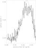 |
Fig. 10 The excesses from the stars #2 and #947 and their corresponding model for the whole spectral range. Photometric measurements are marked with “+” signs, while the spectra are drawn as full drawn lines. The models are marked with “ × ” signs and red lines. |
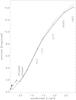 |
Fig. 11 The excesses from the stars #2 and #947 and their corresponding model for the wavelength range λ > 2 μm. Photometric measurements are marked with “+” signs. The spectra are drawn as full drawn lines. The models are marked with “ × ” signs and red lines. |
1.6 and 0.2 respectively. This large difference may not be real, even though it seems plausible that the grain growth inside the globule is mainly due to gas phase carbon and PAH capture onto the graphite grains.
Ice column estimates.
With the column density of the silicates from the grain size distribution, the solar abundance ratio [Si]/[H] (=3.6 × 10⁻⁵), and the assumption, that all silicon are found in the silicates, the column densities N(2· H2 + H) can be found. For the rim of the globule the column density ratio N(2· H2 + H)/AV = 2.3 × 10²¹ and towards the more obscured star the ratio is estimated to be 1.5 × 10²¹. This is in accord with the average column density ratios found for the globule rim earlier (in Paper II).
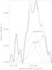 |
Fig. 12 The grain volume distribution as modelled for the rim (probed by star #2) and the central region of B 335 (probed by star #947). The grain size distribution model is a power-law distribution with simple spherical grains of graphite (full lines) and silicates (dashed) with an additional Gaussian grain accumulation at one grain size. |
4.1.2. The extinction curves
So far we have only considered the reddening curves, but now we can use the models to determine the extinction curves, which requires an extrapolation to zero wave number. The two models give A(Ks)/E(I − Ks) = 0.34 for star #947 and 0.13 for star #2. The difference is striking – but is it reasonable? It is clear that the extinction determined towards #2 is more sensitive to systematic effects simply because the obscuration is less and thereby small errors due to how well the model atmosphere represents the true spectrum of the star, how accurate the photometry is calibrated etc will be more important. We also note that there is a small decline in the UV in the reddening curve for #2, which does not seem very likely (this feature is actually causing the sharp peak in the derived graphite grain size distribution). On the other hand, it is interesting to note that both these reddening curves can accurately be represented by the extinction of only graphite and silicate grains with matching size distributions. From this point of view, there is no need for another dust component to explain the well documented slow decline of the reddening curve beyond 2 μm. The dust model for the rim of the cloud is dominated by small grains, which – if it is basically correct – means that there is in fact less extinction at and beyond the K band than previously thought. Consequently, the reason why the reddening curve declines slowly beyond the K band is simply because there is not much extinction left.
As indicated above, the reddening curve for the more obscured star (#947) is better determined and the corresponding extinction model should be trustworthy. In this case, the explanation why the reddening curve declines slowly beyond the K band is the presence of larger (graphite or more general, carbon dominated) grains. This is not very surprising.
4.2. Ices and band strengths
The integrated optical depths, ∫τ(ν)dν, of the water and CO ice bands were calculated. These quantities are directly related to the column densities via 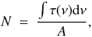 where A is the band strength. Gerakines et al. (1995) have investigated the band strengths for the stretching modes of O-H in water ice at λ = 3.02 μm and C ≡ O in CO ice at λ = 4.67 μm, and found that they are not highly dependent on the pollution from other substances. The resulting column densities of water and CO ice are listed in Table 3.
4.3. CO gas column density
Harjunpää et al. (2004) have observed 13CO and C18O emission from the B 335 globule and in the neighbourhood of the sightline to our background star (A12 in their Table 1) they found a gas N(CO)-column density, that deviates from a linear correlation with the AJ extinction, probably caused by freeze-out of CO. The gas column densities were estimated for the two isotopologues (Table 3), giving slightly different results.
 |
Fig. 13 Detailed view of H2O ice band (fully drawn and a model (dashed) of ice coated grains (with refractive indices from Warren & Brandt 2008). |
Column density and mass ratios observed towards star #947.
4.4. Extinction models for ice coated grains
The ice coatings may either form on the grains by surface reactions or condense onto the surfaces out of the gas phase. In both cases it is reasonable to assume that the ice thickness of the layers is the same for all grain sizes and thus the ice mass is dependent on the size of the grain surface. For water ice we use the refractive index from Warren & Brandt (2008) and using the thickness of the ice layer as a parameter we find a good fit to the measurements as can be seen in Fig. 13. In these calculations we have excluded grains smaller than 25 Å, for which the ice mantles evaporate because of the instant temperature rise when hit by UV photons or cosmic rays (Hollenbach et al. 2009).
The thickness of the coating in combination with the grain size distribution we derived above (see Fig. 12) now allows us to calculate the H2O column density. We note that there is more ice needed (almost a factor 2, see Table 3) to explain the absorption band when we distribute the ice on the grain surfaces than if we simply consider the band strength (which is equivalent to a thin sheet of water ice). We have not looked into the detailed reason for this difference, but it is probably real and if so, all estimates in the literature on column densities of ices are underestimated by about a factor two!
It is interesting to note that the ice coating slightly changes extinction also outside the absorption band and the effect is to lower the extinction, see Fig. 14.
 |
Fig. 14 Influence of H2O ice on the extinction in the optical wavelength range. The ice (dashed) lowers the extinction in the optical from the ice free grain extinction (dotted) line. |
 |
Fig. 15 Detailed view of CO ice extinction and a model (dashed) and the different ices (from Elsila et al. 1997), that have been included. |
For the CO ice the situation is a bit more complicated because the dielectric constants are heavily influenced by the presence of other frozen molecules, like H2O, O2, N2 as well as CO2. Both the peak position and the width of the CO ice band are dependent on the mixture and in an attempt to match the observed band we have optimised for three different mixtures using data from Elsila et al. (1997), see Fig. 15. We realize that this fit cannot be used to claim that e.g. there must be N2 frozen onto the grains – our fit should rather be seen as an example of a possible mixture. However, the calculated column density is not very dependent on the exact mixture and (like in the case of water ice) there is more CO ice needed to explain the absorption band when it is located on dust surfaces than achieved from a direct calculation using the band strength, see Table 3.
Reddening (Aλ − AKs)/E(J − Ks).
5. Discussion
5.1. The reddening curve
As mentioned, the infrared reddening curve for dark clouds has recently been determined in a number of investigations. By assuming the extinction ratio e.g. AH/AK to be the same as for the diffuse ISM (for which it has been determined), the extinction curve follows from:  (1)As we question (see below) the assumption of a more or less universal AH/AK value, we have converted the “extinction” given in these papers back to the reddening as given in Table 5. For comparison we also include the reddening curve for the diffuse ISM determined by Indebetouw et al. (2005). There is a good agreement between the different investigations and the reddening of our star #2, while our result for star #947 differs significantly at the longest wavelengths. For reference we also give the reddening produced by the RV = 5.5 model from Draine (2003a). As has become quite clear during the past decade, the dip in the wavelength range 3–7 μm, predicted by this model is not present in the observations. For this reason, one cannot either trust that it can be used as a link between the near-IR reddening and the absolute extinction (which is frequently assumed).
It is interesting to note that the interstellar reddening of the diffuse ISM does not significantly differ from that of dark clouds, at least until the IRAC 4 band. It is unfortunate, however, that the MIPS 24 band has not yet been included in any investigation of the diffuse ISM.
5.2. The extinction
5.2.1. The diffuse and moderately dense ISM
In Paper II we studied the extinction of the same dark cloud in the optical and near-IR regions based on a large number of stars. We came to the conclusion that the CCM functional form represents the reddening well. However, this does not necessarily mean that the extinction curve is adequately described by the CCM function at these wavelengths. The problem has to do with the extrapolation of the reddening curve to zero wave number. Even though variations of the reddening curve in the near-IR have been noted, it is generally found that the reddening curve can be understood if the extinction in the near-IR follows a power law (Aλ ∝ λ − β), where β = 1.6–1.8 (see Draine 2003b). As cited in the Introduction there is, however, increasing evidence that such a power law is no longer valid beyond 3 μm, and it is therefore not adequate to assume e.g. a AH/AK ratio based on a power law extrapolation. The obvious solution is to extend the observations further into the infrared, and this is the approach of the present paper. However, even if the Spitzer archive allows us to use observations out to 24 μm, the extinction is not zero at this wavelength either. Somehow we must extrapolate to zero wave number. For this purpose we use a grain model designed to fit the reddening curve all the way from the UV to 24 μm, including the important silicate absorption as well as ice features (for the most obscured star). Our grain model is a bit ad hoc (a power law size distribution plus a Gaussian distribution centred on a certain size kept as a parameter in the fitting process), but it is interesting that only silicates and carbon grains (plus ice mantles) are needed to explain the reddening curve(s) from the UV all the way to 24 μm, including the region 3–8 μm. Thus, even though we cannot claim that our grain models are unique, they enable us to extrapolate the reddening curve to zero wave number in a physically reasonable way.
Ideally one would like to measure the relation between the absolute extinction and the reddening without being dependent on a dust model. As discussed in Paper II, star counts offer a way to find the true extinction at a given wavelength, thereby providing the link between the reddening curve and the extinction curve. The main problem in applying this method to dark clouds is their small scale structure. In practice large uncertainties result.
Based on a near-IR survey of the Galactic Bulge, Nishiyama et al. (2006) identify the Red Clump (RC) stars in the colour/magnitude diagrams (CMD) for a large number of sub-fields. Because of variations of the extinction across the field the position in the CMD of the peak of the RC differs from one sub-field to another, and the locus of all these RC peaks directly gives the AKs/E(J − Ks) ratio. Their accuracy is very good: AKs/E(J − Ks) = 0.494 ± 0.006. This is close to our result for star #2: AKs/E(J − Ks) = 0.51. It is also interesting to note that Fritz et al. (2011), who determine the extinction to the galactic centre by measuring the hydrogen recombination lines from 1.28 to 19 μm (relating the absolute scale to the radio continuum and using Menzel’s Case B), get A(Ks)/E(J − Ks) ≈ A(2.16)/(A(1.28) − A(2.16)) = 0.51.
Three different methods thus arrive at the same A(Ks)/E(J − Ks) ratio. All three investigations probe both the diffuse ISM and denser regions, and one may wonder if this result is applicable for the diffuse and/or dense ISM in general. Indebetouw et al. (2005) investigate two directions close to the Galactic plane (l = 042 and l = 284) and get a different result: A(Ks)/E(J − Ks) = 0.67 ± 0.07. Their method is also based on the statistical evidence that red giant stars have a relatively narrow distribution both regarding their near-IR colours and their absolute magnitudes and by assuming that the diffuse interstellar matter is relatively smoothly distributed along the lines of sight, Indebetouw et al. (2005) can interpret the colour/magnitude plots in terms of extinction ratios and the extinction per kpc. They base their analysis on large area surveys, combining 2Mass with Spitzer mapping, and the red giant population is well separated from the dwarf population in their diagrams (see their Fig. 3).
Even though the extinction in our line of sight to star #2 should be dominated by the dark cloud there is also a component of diffuse extinction from the path behind the star. It is therefore of interest to investigate whether e.g. our extinction ratio AJ/AK = 2.96 would deviate by large from the fit to the observed red giant distribution observed by Indebetouw et al. (2005). From their fit they get AJ/AK = 2.5 ± 0.2 and cK = 0.15 ± 0.1. We use the intrinsic colour index and the absolute magnitude of a K1 giant to construct the J versus J − K diagram for such stars along a line of sight. By adjusting the cK value to 0.105 (i.e. well within the error estimates of Indebetouw et al. 2005) we can exactly reproduce the same curve, see Fig. 16. For the corresponding diagram with J versus H − K where we compare the curve based on the result of Indebetouw et al. (2005) (with AH/AK = 1.5 ± 0.1 and cK = 0.15 ± 0.1) we get an identical curve for our value, AH/AK = 1.63, if we use cK = 0.135. This value differs from that we used to make the curves overlap in the previous diagram. If we, as a compromise, use the mean value, cK = 0.12, we still get curves well within the errors quoted by Indebetouw et al. (2005), see Fig. 17.
What does this comparison tell us? It basically illustrates the difficulty to determine the link between the reddening and the extinction curves. Not even such a careful investigation, based on high quality data, as that of Indebetouw et al. (2005), excludes considerably different results for the diffuse ISM (like our result for star #2 or those determined for the path towards the GC by Nishiyama et al. (2006) and Fritz et al. (2011).
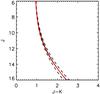 |
Fig. 16 The black curve represents the locus of typical red giant stars at different distances along a line of sight with an extinction of cK = 0.15 kpc-1 and E(J − Ks) = 1.5 ± 0.2 AKs as determined by Indebetouw et al. (2005) for the diffuse ISM. The dashed curves represent the error estimates by these authors. The red curve (on top of the full drawn black curve) represents our determination of star #2 with cK = 0.105 kpc-1 and E(J − Ks) = 1.96 AKs. |
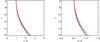 |
Fig. 17 The same assumptions as in Fig. 17. The dashed curves represent the error estimates by these authors. The red curves represents our determination of star #2 with cK = 0.12 kpc-1. The red curves are within the error limits quoted by Indebetouw et al. (2005). This is remarkable in view of the large difference in the E(J − Ks)/AKs and E(H − Ks)/AKs between our result for star #2 (which probes the outer regions of the B 335 globule plus diffuse clouds behind the globule) and the results of Indebetouw et al. (2005). |
5.2.2. Dark clouds
The reddening curve for star #947, sampling dense regions of the B 335 globule, differs considerably at the longest wavelength (24μm) from previous work by Flaherty et al. (2007), Chapman et al. (2009) and Boogert et al. (2011, see Table 5). On the other hand, the results of these authors agree well to ours for star #2, which probes a less dense region than #947. Does it also mean that #947 traces denser regions than those investigated in the cited papers. Flaherty et al. (2007) analyse data from five star formation regions, and there are small differences regarding the reddening in the IRAC bands. For the MIPS 24 μm they present data for two regions, NGC 2068/2071 and the Serpens region. Their background sources probe regions with less extinction than that for #947. Chapman et al. (2009) analyse data from 3 star formation regions and they look separately at regions with different extinctions. Their most obscured stars have extinctions comparable to that of our star #947. Finally, Boogert et al. (2011), who analyse a number of dense cores, certainly include lines of sight with larger extinction than our case study. They determine the spectral classes from IR spectroscopy and use stellar atmosphere models to determine the intrinsic SEDs of the stars. For one of their stars, judged to be well classified, they determine the extinction curve for the continuum assuming the same AKs/E(J − Ks) ratio as determined by Indebetouw. In Table 5 we have removed that assumption to get the reddening curve. Consequently, the reddening curve determined by Boogert et al. (2011) is only based on one star and their method is the same as ours. However, their reddening curve is applied to the 27 other stars and in most cases it fits well, except frequently at the longest wavelength, MIPS 24 μm. It is also at this wavelength where our results differ significantly.
There appears to be a problem to include the MIPS 24 μm fotometric point in a reliable way in these studies. Not only in the large sample of individually studied stars by Boogert et al. (2011) there are many cases which differs significantly from the others. Also in the investigation of Chapman et al. (2009) the less obscured regions exhibit unrealistic values at 24 μm. Assuming that the technical details (colour correction due to the broad filter, the psf correction) have been correctly done in all the cited papers, there remains three sources of error:
- 1.
The MIPS 24 μm photometry is not reproducible enough. According to the MIPS handbook, the repeatability is 1% or better and the absolute calibration is better than 5% determined (using observations of solar type stars, A, and K giant stars). This cannot be the main reason for the apparent problems with the 24 μm photometry.
- 2.
The model atmospheres do not represent the stellar SED well enough for late-type giants. This may well be an issue in particular as the model fits are done with relatively low spectral resolution, preventing an accurate match of metallicity, microturbulence and surface gravity. The most important parameter, Teff, is probably well determined by the combination of photometry and spectroscopy. It should be noted, however, that Boogert et al. (2011) do not use high resolution synthetic spectra for their comparison to the observed spectra – instead they use opacity sampled spectra and degrade the resolution of the observed spectra from R = 2000 to R = 100 for the comparison. This is in our view a waste of information and a likely source of uncertainty.
- 3.
Late type giants are often irregular variables (and, indeed Mira variables). As the observations in the various wavebands are measured at different times, this can cause artificial drops and/or rises in the observed SEDs. There is no indication in the observations of #947 in B 335 that this is the case – actually a smooth SED results even though seven different instruments contribute.
 This value is lower than Boogert et al. (2011) derived from one star in their sample (0.44) and much lower than our value for star #947 (0.84).
Is there a reasonable explanation for this difference? We first note that the estimated error due to classification uncertainty and the photometric accuracy is within the size of the symbol of #947 in Fig. 18, so it should be excluded to explain the exceptional position of this star in the diagram by poor photometry or classification. Even though B 335 is not very far from the galactic plane (b = −6.5), most of the cores investigated by Boogert et al. (2011) are located closer to the galactic plane and/or towards the galactic centre. This means that much of the continuum extinction can be due to the path behind the cores and as a consequence much of the determined E(J − Ks) could be due the diffuse ISM, while most of the mid-IR excess, E(Ks − m(24)) could be caused by the dense cores. Such an explanation might be plausible, but we cannot rule out that our case study of the extinction towards star #947 behind a dense part of B 335 reflects unusual cloud properties.
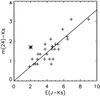 |
Fig. 18 This colour/colour diagram is based on data from an investigation by Boogert et al. (2011) of field stars behind cloud cores. The slope of the curve is well defined, 0.357 ± 0.013. The asterisk represents the star #947 in our investigation, and it is clearly different from the general trend. |
6. Conclusions
Based on photometry in the range 0.35–24 μm as well as IR spectroscopy we determine the reddening curve towards stars behind the dark globule B 335. For the most obscured star we also determine the absorption bands due to water ice, CO ice and silicates. We confirm earlier findings that the reddening curve levels off beyond the K band in contrast to current models (e.g. Weingartner & Draine 2001). From the reddening curve we also draw the following conclusions concerning the grain size distribution, the extinction and the ice bands.
Grain size distribution The grain size distribution features. Based on a relatively simple assumption for the grain size distribution (a power law and a Gaussian) for silicate and graphite grains we find solutions that closely match the observed reddening curves for the two background stars for which we have silicate band observations. One of the stars probe the central part of the globule and the other the rim. For the most obscured star the model fit has a peak of graphite grains at a radius of 2 μm, while the graphite peak for the other star is at 0.5 μm. In neither case there is any need for an additional grain material to explain the reddening curve. The abundance ratio graphite/slicates differs substantially for the two models (much more graphite in the central region). As a consequence we have two different explanations of the shallow reddening curve beyond the K band: for the denser region it is because of larger graphite or, more general, carbon grains which give rise to a higher mid-IR extinction than predicted by previous models constructed to match the UV to near-IR spectral range (cf. Weingartner & Draine 2001). For the outer region of the globule the explanation is simply that the extinction as such is low beyond the K band. Actually, much of the extinction towards the stars at the rim of the globule may originate in the diffuse medium beyond the cloud, and we suggest that this explanation to the shallow reddening curve beyond the K band is valid not only for the outer regions of the cloud but also for the diffuse ISM. Gas column density. The column densities ratios N(2·H2 + H)/AV are estimated to be 2.3 × 10²¹ for the lower extinction sightline and 1.5 × 10²¹ for the higher extinction sightline. Extinction model The extinction model for the outer part of B 335 gives the relation AKs = 0.51·E(J − Ks). This latter relation agrees with recent determinations towards the galactic centre by Nishiyama et al. (2006) and Fritz et al. (2011) using different methods. Indebetouw et al. (2005) get a higher value for the diffuse ISM, AKs = 0.67·E(J − Ks), but we show that this difference is not significant and conclude that AKs ≈ 0.51·E(J − Ks) for the diffuse ISM as well as for moderately dense molecular regions. The extinction model for the denser part of the B 335 gives the relation AKs = 0.97·E(J − Ks). Although this model describes the reddening curve from the UV to 24 μm, including the silicate, the water-ice, and the CO-ice bands well, we have indications that it represents conditions that may be different from other dense cores. Ice bands The water ice band is reproduced by grains coated with pure water ice. The column density of water ice is half of that found in the Taurus clouds (Whittet et al. 2001’s) for the same extinction. The difference is likely due to a larger interstellar radiation field in the B 335 region, desorbing ice mantles deeper in the cloud. The CO ice band differs in position from that of pure CO ice mantles, indicating that CO is mixed in other ices. Based on published laboratory measurements of frozen gas mixtures we show that the CO ice band can be understood if CO is part of such mixtures (where H2O is a natural part and N2 a possible part). The ice/gas ratio is relatively high (0.8–1.) and as this is an average along the AJ = 3.5 cloud extinction towards the probing star and as we must allow for relatively deep regions free from CO ice on both the front and the rear side of the cloud, the ice/gas CO ratio must be greater than unity in the interior of the cloud, and more than half of the gas is depleted. This confirms earlier findings (Bacmann et al. 2002) that CO (or CO isotopologues) cannot be used as a mass tracer in dense and cold molecular clouds. The CO2 ice band at 15.2 μm indicated in the ISOCAM-CVF spectrum is not confirmed in the Spitzer spectra and we can only give an upper limit to the CO2-ice column density.
Acknowledgments
This publication makes use of data products from the Two Micron All Sky Survey, which is a joint project of the University of Massachusetts and the Infrared Processing and Analysis Center/California Institute of Technology, funded by the National Aeronautics and Space Administration and the National Science Foundation. This work is based [in part] on archival data obtained with the Spitzer Space Telescope, which is operated by the Jet Propulsion Laboratory, California Institute of Technology under a contract with NASA.
References
- Bacmann, A., Lefloch, B., Ceccarelli, C., et al. 2002, A&A, 389, L6 [NASA ADS] [CrossRef] [EDP Sciences] [Google Scholar]
- Boogert, A. C. A., Huard, T. L., Cook, A. M., et al. 2011, ApJ, 729, 92 [NASA ADS] [CrossRef] [Google Scholar]
- Cardelli, J. A., Clayton, G. C., & Mathis, J. S. 1989, ApJ, 345, 245 [NASA ADS] [CrossRef] [Google Scholar]
- Chapman, N. L., Mundy, L. G., Lai, S., & Evans, N. J. 2009, ApJ, 690, 496 [NASA ADS] [CrossRef] [Google Scholar]
- Chiar, J. E., Pendleton, Y. J., Allamandola, L. J., et al. 2011, ApJ, 731, 9 [NASA ADS] [CrossRef] [Google Scholar]
- Draine, B. T. 2003a, ArXiv Astrophysics e-prints [Google Scholar]
- Draine, B. T. 2003b, ARA&A, 41, 241 [NASA ADS] [CrossRef] [Google Scholar]
- Draine, B. T. 2003c, ApJ, 598, 1017 [NASA ADS] [CrossRef] [Google Scholar]
- Draine, B. T., & Lee, H. M. 1984, ApJ, 285, 89 [Google Scholar]
- Elsila, J., Allamandola, L. J., & Sandford, S. A. 1997, ApJ, 479, 818 [NASA ADS] [CrossRef] [PubMed] [Google Scholar]
- Flaherty, K. M., Pipher, J. L., Megeath, S. T., et al. 2007, ApJ, 663, 1069 [CrossRef] [Google Scholar]
- Fritz, T. K., Gillessen, S., Dodds-Eden, K., et al. 2011, ApJ, 737, 73 [NASA ADS] [CrossRef] [Google Scholar]
- Gerakines, P. A., Schutte, W. A., Greenberg, J. M., & van Dishoeck, E. F. 1995, A&A, 296, 810 [NASA ADS] [Google Scholar]
- Gibb, E. L., Whittet, D. C. B., Boogert, A. C. A., & Tielens, A. G. G. M. 2004, ApJS, 151, 35 [NASA ADS] [CrossRef] [PubMed] [Google Scholar]
- Harjunpää, P., Lehtinen, K., & Haikala, L. K. 2004, A&A, 421, 1087 [NASA ADS] [CrossRef] [EDP Sciences] [Google Scholar]
- Hauschildt, P. H., Allard, F., Ferguson, J., Baron, E., & Alexander, D. R. 1999, ApJ, 525, 871 [NASA ADS] [CrossRef] [Google Scholar]
- Hollenbach, D., Kaufman, M. J., Bergin, E. A., & Melnick, G. J. 2009, ApJ, 690, 1497 [CrossRef] [Google Scholar]
- Indebetouw, R., Mathis, J. S., Babler, B. L., et al. 2005, ApJ, 619, 931 [NASA ADS] [CrossRef] [Google Scholar]
- Knez, C., Boogert, A. C. A., Pontoppidan, K. M., et al. 2005, ApJ, 635, L145 [NASA ADS] [CrossRef] [Google Scholar]
- Mathis, J. S., Rumpl, W., & Nordsieck, K. H. 1977, ApJ, 217, 425 [NASA ADS] [CrossRef] [Google Scholar]
- Nishiyama, S., Nagata, T., Kusakabe, N., et al. 2006, ApJ, 638, 839 [NASA ADS] [CrossRef] [Google Scholar]
- Olofsson, S., & Olofsson, G. 2009, A&A, 498, 455 [NASA ADS] [CrossRef] [EDP Sciences] [Google Scholar]
- Olofsson, S., & Olofsson, G. 2010, A&A, 522, A84 [NASA ADS] [CrossRef] [EDP Sciences] [Google Scholar]
- Pontoppidan, K. M., Fraser, H. J., Dartois, E., et al. 2003, A&A, 408, 981 [NASA ADS] [CrossRef] [EDP Sciences] [Google Scholar]
- Rieke, G. H., & Lebofsky, M. J. 1985, ApJ, 288, 618 [NASA ADS] [CrossRef] [Google Scholar]
- Román-Zúñiga, C. G., Lada, C. J., Muench, A., & Alves, J. F. 2007, ApJ, 664, 357 [NASA ADS] [CrossRef] [Google Scholar]
- Skrutskie, M. F., Cutri, R. M., Stiening, R., et al. 2006, AJ, 131, 1163 [NASA ADS] [CrossRef] [Google Scholar]
- Warren, S. G., & Brandt, R. E. 2008, J. Geophys. Res. (Atmospheres), 113, 14220 [Google Scholar]
- Weingartner, J. C., & Draine, B. T. 2001, ApJ, 548, 296 [NASA ADS] [CrossRef] [Google Scholar]
- Whittet, D. C. B., Gerakines, P. A., Hough, J. H., & Shenoy, S. S. 2001, ApJ, 547, 872 [NASA ADS] [CrossRef] [Google Scholar]
All Tables
All Figures
|
Fig. 1 A U band image of the B335 globule. The centre YSO and its outflow region as well as the background stars are marked. The circle represents the position of the 13CO and the C18O measurement closest to the background star #947 in Harjunpää et al. (2004) and the size of the circle represents the 45′′ beam width. |
| In the text | |
|
Fig. 2 The optical and near-IR extinctions towards the background stars #947 and #90. The extinction for #90 and #947 are well represented by the fitted CCM-extinction with RV = 4.9 (dashed). |
| In the text | |
|
Fig. 3 The optical spectrum of the most obscured star (#947) is well represented by a stellar model (from Hauschildt et al. 1999) with Teff 3050 K. The stellar model (red curve) has been modified by a weighting function ∝ λ-1 to account for the interstellar reddening. |
| In the text | |
|
Fig. 4 The ISAAC spectrum in the L band of star #947 (blue curve) and the stellar atmospheric model (red curve) are divided to get the water ice band (black curve). |
| In the text | |
|
Fig. 5 The ISAAC spectrum in the M band of star #947 (blue curve) and the corresponding stellar atmospheric model (red curve) are divided to get the CO ice band (black curve). |
| In the text | |
|
Fig. 6 Spectra for sight lines towards stars #2 (lower) and #947 (upper curve) as observed by Spitzer-IRS (#2: 7 < λ < 14 μm) and ISOCAM-CVF (#947: 5 < λ < 16 μm) and photometry from Spitzer-IRAC and Spitzer-MIPS (+ signs). |
| In the text | |
|
Fig. 7 The optical depth of the silicate band τsilicate towards star #2 (dashed line) and #947 (full line) as determined from Spitzer-IRS and ISOCAM-CVF observations, respectively. Although the S/N of the observations does not allows for an interpretation of the details, we note that for star #947 the band peaks at ≈ 0.109 μm-1 corresponding to 9.2 μm. |
| In the text | |
|
Fig. 8 The “reddening” curve in the mid-IR, “normalized excess” = E(λ − Ks)/E(I − Ks) vs. wave number, for six stars behind the B 335 globule. The normalized excess derived from the Spitzer/ISOCAM spectra of two of the stars, #2 and # 947, are included with the same normalization. |
| In the text | |
|
Fig. 9 The normalized excess, (E(λ − Ks)/E(I − Ks), in the mid-IR for the weighted average of the five stars at the rim of the B 335 globule (blue) and the most obscured star (red). The green curve represents the Draine (2003a)RV = 5.5 curve. |
| In the text | |
|
Fig. 10 The excesses from the stars #2 and #947 and their corresponding model for the whole spectral range. Photometric measurements are marked with “+” signs, while the spectra are drawn as full drawn lines. The models are marked with “ × ” signs and red lines. |
| In the text | |
|
Fig. 11 The excesses from the stars #2 and #947 and their corresponding model for the wavelength range λ > 2 μm. Photometric measurements are marked with “+” signs. The spectra are drawn as full drawn lines. The models are marked with “ × ” signs and red lines. |
| In the text | |
|
Fig. 12 The grain volume distribution as modelled for the rim (probed by star #2) and the central region of B 335 (probed by star #947). The grain size distribution model is a power-law distribution with simple spherical grains of graphite (full lines) and silicates (dashed) with an additional Gaussian grain accumulation at one grain size. |
| In the text | |
|
Fig. 13 Detailed view of H2O ice band (fully drawn and a model (dashed) of ice coated grains (with refractive indices from Warren & Brandt 2008). |
| In the text | |
|
Fig. 14 Influence of H2O ice on the extinction in the optical wavelength range. The ice (dashed) lowers the extinction in the optical from the ice free grain extinction (dotted) line. |
| In the text | |
|
Fig. 15 Detailed view of CO ice extinction and a model (dashed) and the different ices (from Elsila et al. 1997), that have been included. |
| In the text | |
|
Fig. 16 The black curve represents the locus of typical red giant stars at different distances along a line of sight with an extinction of cK = 0.15 kpc-1 and E(J − Ks) = 1.5 ± 0.2 AKs as determined by Indebetouw et al. (2005) for the diffuse ISM. The dashed curves represent the error estimates by these authors. The red curve (on top of the full drawn black curve) represents our determination of star #2 with cK = 0.105 kpc-1 and E(J − Ks) = 1.96 AKs. |
| In the text | |
|
Fig. 17 The same assumptions as in Fig. 17. The dashed curves represent the error estimates by these authors. The red curves represents our determination of star #2 with cK = 0.12 kpc-1. The red curves are within the error limits quoted by Indebetouw et al. (2005). This is remarkable in view of the large difference in the E(J − Ks)/AKs and E(H − Ks)/AKs between our result for star #2 (which probes the outer regions of the B 335 globule plus diffuse clouds behind the globule) and the results of Indebetouw et al. (2005). |
| In the text | |
|
Fig. 18 This colour/colour diagram is based on data from an investigation by Boogert et al. (2011) of field stars behind cloud cores. The slope of the curve is well defined, 0.357 ± 0.013. The asterisk represents the star #947 in our investigation, and it is clearly different from the general trend. |
| In the text | |
Current usage metrics show cumulative count of Article Views (full-text article views including HTML views, PDF and ePub downloads, according to the available data) and Abstracts Views on Vision4Press platform.
Data correspond to usage on the plateform after 2015. The current usage metrics is available 48-96 hours after online publication and is updated daily on week days.
Initial download of the metrics may take a while.