| Issue |
A&A
Volume 533, September 2011
|
|
|---|---|---|
| Article Number | A43 | |
| Number of page(s) | 5 | |
| Section | Stellar structure and evolution | |
| DOI | https://doi.org/10.1051/0004-6361/201117252 | |
| Published online | 24 August 2011 | |
Gravity darkening in rotating stars
1
Université de Toulouse, UPS-OMP, IRAP, Toulouse France
e-mail: This email address is being protected from spambots. You need JavaScript enabled to view it.
2
CNRS, IRAP, 14, avenue Edouard Belin, 31400 Toulouse, France
Received: 13 May 2011
Accepted: 13 July 2011
Abstract
Context. Interpretation of interferometric observations of rapidly rotating stars requires a good model of their surface effective temperature. Until now, laws of the form  have been used, but they are only valid for slowly rotating stars.
Aims. We propose a simple model that can describe the latitudinal variations in the flux of rotating stars at any rotation rate.
Methods. This model assumes that the energy flux is a divergence-free vector that is antiparallel to the effective gravity.
Results. When mass distribution can be described by a Roche model, the latitudinal variations in the effective temperature only depend on a single parameter, namely the ratio of the equatorial velocity to the Keplerian velocity. We validate this model by comparing its predictions to those of the most realistic two-dimensional models of rotating stars issued from the ESTER code. The agreement is very good, as it is with the observations of two rapidly rotating stars, α Aql and α Leo.
Conclusions. We suggest that as long as a gray atmosphere can be accepted, the inversion of data on flux distribution coming from interferometric observations of rotating stars uses such a model, which has just one free parameter.
Key words: stars: atmospheres / stars: rotation
© ESO, 2011
1. Introduction
The recent development of long-baseline optical/infrared interferometry has allowed direct observation of gravity darkening at the surface of some rapidly rotating stars. This phenomenon has been known since the work of von Zeipel (1924), who noticed that the radiative flux is proportional to the effective gravity geff in a barotropic star (i.e. when the pressure only depends on the density). Thus, the effective temperature Teff varies with latitude, following  . This is known as the von Zeipel law.
Barotropicity, however, is a strong hypothesis, and is actually incompatible with a radiative zone in solid body rotation. This problem was noticed by Eddington (1925) and has led to many discussions over subsequent decades (see Rieutord 2006, for a review). Now, the recent interferometric observations of some nearby rapidly rotating stars by McAlister et al. (2005), Aufdenberg et al. (2006), van Belle et al. (2006), and Zhao et al. (2009) have shown that gravity darkening is not well represented by von Zeipel’s law, which seems to overestimate the temperature difference between pole and equator. This conclusion is usually expressed using a power law, , with an exponent less than 1/4. This is traditionally explained by the existence of a thin convective layer at the surface of the star, in reference to the work of Lucy (1967), who found β ~ 0.08 for stars with a convective envelope.
Actually, the weaker variation in the flux with latitude, compared to von Zeipel’s law has also been noticed by Lovekin et al. (2006), Espinosa Lara & Rieutord (2007), and Espinosa Lara (2010) in two-dimensional numerical models of rotating stars. This prompted us to reexamine this question using these new models. It leads us to a new approach that avoids the strong assumption of von Zeipel and that is presumably able to better represent the gravity darkening of fast rotating stars. This paper aims at presenting this new model.
In Sect. 2 we explain the derivation of the new model of gravity darkening and the associated assumptions. In the next section, results are compared to the values of two-dimensional models and to observations. Conclusions follow.
2. The model
Before presenting our model, we briefly recall the origin of the von Zeipel law and Lucy’s exponent. In a radiative region the flux is essentially carried by the diffusion of photons and thus correctly described by Fourier’s law, 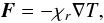 (1)where χr is the radiative heat conductivity. If the star is assumed to be barotropic, density and temperature (and thus χr) are only functions of the total potential Φ (gravitational plus centrifugal). Hence,
  (2)If we define the surface of the star as a place of constant given optical depth, we see that this model implies latitudinal variations in the flux that strictly follow those of the effective gravity. Using the effective temperature, we recover .
Lucy’s approach is based on a first-order development of the dependence between Teff and geff in a convective envelope. Since the convective flux is almost orthogonal to isentropic surfaces, log Teff and log geff are related on such a surface. Deep enough where the entropy is almost the same everywhere, s(log Teff,log geff) = s0, where s0 is the specific entropy in the bulk of the convection zone. Assuming that at first order, one finds that  (3)at zero rotation. Lucy (1967) computed this exponent for various stellar models and found that is was weakly dependent on the mass, radius, luminosity, or chemical abundance of the model. The mean value β ~ 0.08 was thus proposed.
From the foregoing recap, we should remember that both approaches are based on assumptions that require a small deviation from sphericity, and thus they demand slow rotation.
2.1. Hypothesis for a new model
It is quite clear from observations that slow rotation is not appropriate when dealing with observed gravity darkenings. We recall that Altair (α Aql), a favorite target of interferometry (Domiciano de Souza et al. 2005; Peterson et al. 2006a; Monnier et al. 2007) is thought to be rotating close to 90% of the breakup angular velocity. Thus any modeling of its gravity darkening should be able to deal with rapid rotation.
We propose to assume that the flux in the envelope of a rotating star is very close to 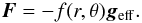 (4)Here, f is some function of the position to be determined where r, θ, and ϕ are the spherical coordinates. In doing so, we hypothesize that the energy flux vector is almost antiparallel to the effective gravity. This is justified in a convective envelope where heat transport is essentially in the vertical direction, following buoyancy. In radiative regions, the flux is antiparallel to the temperature gradient, which is slightly off the potential gradient because of baroclinicity. Fortunately, the angle between the two vectors remains very small, even in the case of extreme rotation. As shown by Fig. 1, a two-dimensional stellar model with rotation at 90% of the break-up velocity gives an angle between ∇T and geff of less than half a degree (i.e. less than 10-2 rd). Comparing our model to that of von Zeipel, we see that it does not imply that latitudinal variations of the flux are the same as those of the effective gravity or, equivalently, it allows the ratio F/geff to vary with latitude.
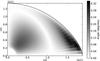 |
Fig. 1 Meridional cut representing the angle (in degrees) formed by the pressure gradient and the energy flux in a 3 M⊙ star rotating at 90% of its Keplerian velocity at the equator calculated using the ESTER code. |
In the envelope of a star, where no heat is generated, we have  (5)or
(5)or  (6)This equation is completed by an appropriate boundary condition (see below). Presently, we need to note that the solution only depends on the effective potential, that is, on the mass distribution. Such a quantity is generally not known, but we may observe that rapidly rotating stars are usually massive or intermediately massive, hence rather centrally condensed. We therefore chose the Roche model to represent the mass distribution. Its simplicity is also attractive. We thus set
 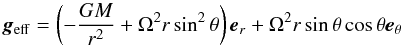 (7)where er and eθ are radial unit vectors associated with the spherical coordinates.
According to this model 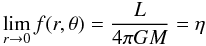 (8)where L is the luminosity of the star, M its mass, and η is actually the constant that scales the function f. We therefore write
 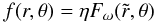 (9)where
 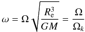 (10)is the nondimensional measure of the rotation rate where Ωk is the Keplerian angular velocity at the equator, and
  the dimensionless radial coordinate scaled by the equatorial radius Re. We see that in this model the latitude dependence of the flux is controlled by a single parameter ω. It is therefore as easy to use as the previous models of von Zeipel or Lucy, but it is likely to be much more robust at high rotation.
2.2. Solution of the new model
For the Roche model ∇·geff = 2Ω2, so the dimensionless form of Eq. (6) can be written as 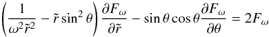 (11)with the boundary condition
  (12)This linear, first-order, and homogeneous partial differential equation can be solved by using a change of variable based on the method of characteristics. Along a characteristic curve of (11) we have
  (13)We can multiply the first and second terms by an arbitrary function
 (14)which leads to
 ![Mathematical equation: \begin{equation} \label{dtau} G(\tilde r,\theta)\left[\sin\theta\cos\theta\mathrm{d}\tilde r+\left(\frac{1}{\omega^2\tilde r^2} -\tilde r\sin^2\theta\right)\mathrm{d}\theta\right]=0=\mathrm{d}\tau, \end{equation}](/articles/aa/full_html/2011/09/aa17252-11/aa17252-11-eq49.png) (15)where we have defined a new variable τ that will be constant along a characteristic curve.
(15)where we have defined a new variable τ that will be constant along a characteristic curve.
Without loss of generality we choose1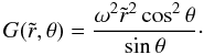 (16)This leads, via the chain rule
  , to a system of differential equations to calculate τ
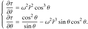 (17)From the first equation we obtain
 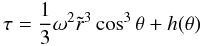 (18)with h(θ) an unknown function. Using (18) in the second equation of (17), we find
 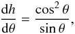 (19)which can be integrated, yielding
 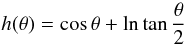 (20)so that (18) becomes
 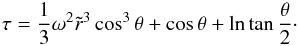 (21)In fact, the curves τ = const. are the streamlines of the flux F, hence also those of the effective gravity geff according to Eq. (4).
After making the change of variable  , the original differential Eq. (11) simplifies to (also from Eq. (13))
 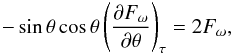 (22)which can be solved to get the general solution
 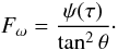 (23)The function ψ(τ) can be calculated using the boundary condition (12). We define a new variable
  such that
 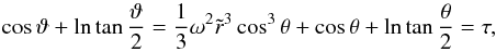 (24)so that ϑ ≡ ϑ(τ). For a given value of τ, ϑ is the corresponding value of θ when
  . From Eq. (23) we easily find that
 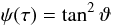 (25)and
 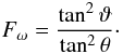 (26)This expression can be used to calculate the energy flux everywhere in the star. However, we may note singularities at θ = 0 and θ = π/2, i.e. at the pole and the equator of the star. Actually, these points are not real singularities since the direct resolution of Eq. (11) at these points gives
 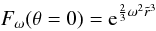 (27)and
 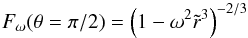 (28)using the boundary condition (12).
2.3. The effective temperature profile
To obtain the latitudinal profile of Teff at the surface of the star, one must proceed as follows. Once ω is fixed, the shape of the surface  is given by the Roche potential
 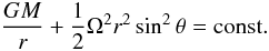 (29)Using Eq. (10), it follows that
  is the solution of
 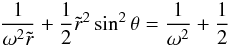 (30)for a given θ. Thus the value of ϑ at each point on the surface (
 ) can be calculated using (24). This equation is efficiently solved with an iterative method like the Newton one. Then we have
  (31)which shows that the temperature profile depends on a single parameter ω. As a consequence the ratio of equatorial to polar effective temperature is, when using (27) and (28), given by
 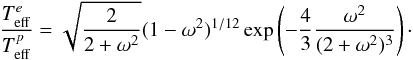 (32)Finally we note that von Zeipel’s law is recovered at slow rotation, since in this case ϑ ≃ θ and Eq. (31) simplifies into
  (33)
(33)
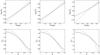 |
Fig. 2 Comparison between the gravity darkening profile calculated using the model described in Sect. 2.3 (solid line), using von Zeipel’s law (dashed line), and the models calculated using the ESTER code (crosses). Left: star with M = 3 M⊙ and homogeneous composition rotating at 70% of the Keplerian velocity at the equator (Ωk). Center: M = 3 M⊙, Ω = 0.7Ωk and with hydrogen abundance in the core Xc = 0.5X, with X the abundance in the envelope. Right: same as center but with Ω = 0.9Ωk. In the bottom row θ is the colatitude. |
3. Results and comparison with ESTER models
To validate the foregoing model of gravity darkening, we compare its results to those of fully two-dimensional models of rotating stars produced by the ESTER2 code (e.g. Espinosa Lara & Rieutord 2007; Rieutord & Espinosa Lara 2009; Espinosa Lara 2010). These models utilize the OPAL opacities and equation of state (Iglesias & Rogers 1996; Rogers et al. 1996). They include a convective core and a fully radiative envelope. They are presently calculated in the limit of vanishing viscosity, which requires a prescription for the differential rotation. Here, we have chosen the surface rotation to be solid. The interior rotation is then self-consistently derived.
We have computed two sets of models. The first set has homogeneous composition with masses between 2.5 M⊙ and 4 M⊙ and the full range of rotation velocities, from zero up to the breakup velocity. The second set covers the same range of masses and velocities, but we have set the hydrogen abundance in the core to be 50% of the abundance in the envelope. This results in a smaller core compared to the size of the star.
Figure 2 shows the comparison between our model of gravity darkening and the stellar models calculated using the ESTER code. It represents the profile of effective temperature as a function of surface effective gravity (top) and colatitude (bottom). The normalized values are defined as  and
and  . For comparison, we have also plotted the profile predicted by von Zeipel’s law. The first two columns on the left show the results for a star rotating at 70% of the Keplerian velocity at the equator3 Ωk, while the third one corresponds to Ω = 0.9Ωk. The difference between the first and the second columns is the hydrogen abundance in the core. As we observe, von Zeipel’s law systematically overestimates the ratio between polar and equatorial effective temperature, while there is good agreement between the predictions of Fω and the ESTER models. The same behavior can be seen in Fig. 3, which shows the ratio between equatorial and polar effective temperature as a function of the flattening of the star ϵ = 1 − Rp/Re, even at high rotation rates.
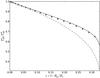 |
Fig. 3 Ratio between equatorial and polar effective temperature as a function of flattening ϵ = 1 − Rp/Re. Solid line: the analytical model presented in this paper. Dashed line: Von Zeipel’s law. Crosses: ESTER models of set 1 (Xc = X). Triangles: ESTER models of set 2 (Xc = 0.5X). |
The good agreement between the profile of the effective temperature predicted by the new model and the output of the ESTER code is general. However, there are some slight deviations, which are more important for the models with homogeneous composition. We think that this may be a consequence of the differential rotation of ESTER models, which contain a convective core rotating faster than the envelope. This leads to a different shape of equipotential surfaces (or isobars) compared to the rigidly rotating Roche model that is used in the simple model. This difference is less important for “evolved” models, because they have smaller cores.
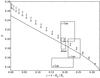 |
Fig. 4 Gravity darkening coefficient β as a function of flattening. The values were calculated using a least-square fit to the profile of effective temperature. Solid line: model presented in this paper. Crosses: ESTER models of set 1 (Xc = X). Triangles: ESTER models of set 2 (Xc = 0.5X). The corresponding value of β for von Zeipel’s law is 0.25. The boxes represent the values of β, with their corresponding errors, obtained by interferometry for several rotating stars: Altair (Monnier et al. 2007), α Cephei (Zhao et al. 2009), β Cassiopeiae, and α Leonis (Che et al. 2011). |
The gravity darkening exponent β, derived from a generalization of von Zeipel’s law  , is commonly used in observational work to measure the strength of gravity darkening. In Fig. 2 we can observe that the relation between effective temperature and gravity is not exactly a power law. Using such a law is therefore not quite appropriate, but since β-exponents have been derived from observations, we feel it is worth deriving a best-fit exponent associated with ESTER models. These are shown in Fig. 4. This plot clearly shows that the value β = 0.25 given by von Zeipel’s law is appropriate only in the limit of slow rotation as expected. In this figure we also plotted measurements of the gravity darkening exponent β derived by interferometry for several rapidly rotating stars, Altair (Monnier et al. 2007), α Cephei (Zhao et al. 2009), β Cassiopeiae, and α Leonis (Che et al. 2011). We can see that there is good (Altair, α Leo) or fair (α Cep) agreement between the observed values and the model. The discrepancy for β Cas may come from its small inclination angle (~20 deg), so we see the star near pole-on, which makes determining of its flattening more difficult and makes the results depend more on the model used for gravity darkening and limb darkening.
4. Conclusions
Observing that the energy radiated by a star is produced almost entirely in the stellar core and that most stars may be considered close to a steady state, we have noted that the energy flux is essentially a divergence-free vector field. We also observed from full two-dimensional models of rotating stars that the direction of this vector is always very close to that of the effective gravity, so it only depends on the mass distribution. Following this picture, the physical conditions in the outer layers can only affect the flux radiated outside the star very slightly as long as a gray atmosphere can be assumed. Thus, we proposed that the energy flux in the envelope of a rotating star be approximated by  .
.
We have shown how the non-dimensional function Fω(r,θ) can be evaluated by assuming that mass distribution is represented by the Roche model. We then demonstrated that the latitudinal variation of the effective temperature only depends on a single parameter  . Such a model is very appropriate to interpreting the interferometric observations of rotating stars since, unlike von Zeipel’s or Lucy’s laws, it is valid for high rotation rates (up to breakup) and depends only on a single parameter (the β-exponent is removed). Adjustment of the observed surface flux would thus only require variations in ω and i, the inclination of the rotation axis on the line of sight.
As previously mentioned, this model fits the fully 2D models well using a gray atmosphere with a rigidly rotating surface (but with interior differential rotation). This dynamical feature of the models may not be very realistic, so we tested a surface rotation Ω(θ) = Ωeq(1 − 0.1cos2θ) inspired by observations (Collier Cameron 2007). The difference is hardly perceptible, therefore the proposed model of gravity darkening looks quite robust. Future improvement of two-dimensional models will of course be used to confirm this robustness.
The function is in fact an integrating factor that should be chosen so that Eq. (15) is an exact differential, namely that  ; then a solution
  exists. This form is not unique since any function of τ will also be a solution.
Evolution STEllaire en Rotation.
Although Keplerian velocity  can be identified as the critical velocity, we use the former term to avoid confusion with other definitions of critical velocity seen in most works. A common definition is based on a series of models (typically Roche models) of increasing rotation rate, in which the critical velocity Ωc is defined as the angular velocity of the model rotating at the break-up limit. For Roche models,
  . These definitions are not equivalent, a star with Ω = 0.7Ωk will have Ω ≃ 0.93Ωc.
Acknowledgments
The authors acknowledge the support of the French Agence Nationale de la Recherche (ANR), under grant ESTER (ANR-09-BLAN-0140). This work was also supported by the Centre National de la Recherche Scientifique (C.N.R.S., UMR 5572), through the Programme National de Physique Stellaire (P.N.P.S.). The numerical calculations were carried out on the CalMip machine of the “Centre Interuniversitaire de Calcul de Toulouse” (CICT), which is gratefully acknowledged.
References
- Aufdenberg, J. P., Mérand, A., Coudé du Foresto, V., et al. 2006, ApJ, 645, 664 [NASA ADS] [CrossRef] [Google Scholar]
- Che, X., Monnier, J. D., Zhao, M., et al. 2011, ApJ, 732, 68 [NASA ADS] [CrossRef] [Google Scholar]
- Collier Cameron, A. 2007, Astron. Nachr., 328, 1030 [NASA ADS] [CrossRef] [Google Scholar]
- Domiciano de Souza, A., Kervella, P., Jankov, S., et al. 2005, A&A, 442, 567 [NASA ADS] [CrossRef] [EDP Sciences] [Google Scholar]
- Eddington, A. S. 1925, The Observatory, 48, 73 [NASA ADS] [Google Scholar]
- Espinosa Lara, F. 2010, Ap&SS, 328, 291 [Google Scholar]
- Espinosa Lara, F., & Rieutord, M. 2007, A&A, 470, 1013 [NASA ADS] [CrossRef] [EDP Sciences] [Google Scholar]
- Iglesias, C. A., & Rogers, F. J. 1996, ApJ, 464, 943 [NASA ADS] [CrossRef] [Google Scholar]
- Lovekin, C. C., Deupree, R. G., & Short, C. I. 2006, ApJ, 643, 460 [NASA ADS] [CrossRef] [Google Scholar]
- Lucy, L. B. 1967, ZAp, 65, 89 [NASA ADS] [Google Scholar]
- McAlister, H. A., ten Brummelaar, T. A., Gies, D. R., et al. 2005, ApJ, 628, 439 [NASA ADS] [CrossRef] [Google Scholar]
- Monnier, J. D., Zhao, M., Pedretti, E., et al. 2007, Science, 317, 342 [NASA ADS] [CrossRef] [PubMed] [Google Scholar]
- Peterson, D., Hummel, C., Pauls, T., et al. 2006a, ApJ, 636, 1087 [NASA ADS] [CrossRef] [Google Scholar]
- Rieutord, M. 2006, in Stellar Fluid dynamics and numerical simulations: From the Sun to Neutron Stars, ed. M. Rieutord, & B. Dubrulle, EAS Publ., 21, 275 [Google Scholar]
- Rieutord, M., & Espinosa Lara, F. 2009, Comm. Asteroseismol., 158, 99 [Google Scholar]
- Rogers, F. J., Swenson, F. J., & Iglesias, C. A. 1996, ApJ, 456, 902 [NASA ADS] [CrossRef] [Google Scholar]
- van Belle, G. T., Ciardi, D. R., ten Brummelaar, T., et al. 2006, ApJ, 637, 494 [NASA ADS] [CrossRef] [Google Scholar]
- von Zeipel, H. 1924, MNRAS, 84, 665 [NASA ADS] [CrossRef] [Google Scholar]
- Zhao, M., Monnier, J. D., Pedretti, E., et al. 2009, ApJ, 701, 209 [NASA ADS] [CrossRef] [Google Scholar]
All Figures
|
Fig. 1 Meridional cut representing the angle (in degrees) formed by the pressure gradient and the energy flux in a 3 M⊙ star rotating at 90% of its Keplerian velocity at the equator calculated using the ESTER code. |
| In the text | |
|
Fig. 2 Comparison between the gravity darkening profile calculated using the model described in Sect. 2.3 (solid line), using von Zeipel’s law (dashed line), and the models calculated using the ESTER code (crosses). Left: star with M = 3 M⊙ and homogeneous composition rotating at 70% of the Keplerian velocity at the equator (Ωk). Center: M = 3 M⊙, Ω = 0.7Ωk and with hydrogen abundance in the core Xc = 0.5X, with X the abundance in the envelope. Right: same as center but with Ω = 0.9Ωk. In the bottom row θ is the colatitude. |
| In the text | |
|
Fig. 3 Ratio between equatorial and polar effective temperature as a function of flattening ϵ = 1 − Rp/Re. Solid line: the analytical model presented in this paper. Dashed line: Von Zeipel’s law. Crosses: ESTER models of set 1 (Xc = X). Triangles: ESTER models of set 2 (Xc = 0.5X). |
| In the text | |
|
Fig. 4 Gravity darkening coefficient β as a function of flattening. The values were calculated using a least-square fit to the profile of effective temperature. Solid line: model presented in this paper. Crosses: ESTER models of set 1 (Xc = X). Triangles: ESTER models of set 2 (Xc = 0.5X). The corresponding value of β for von Zeipel’s law is 0.25. The boxes represent the values of β, with their corresponding errors, obtained by interferometry for several rotating stars: Altair (Monnier et al. 2007), α Cephei (Zhao et al. 2009), β Cassiopeiae, and α Leonis (Che et al. 2011). |
| In the text | |
Current usage metrics show cumulative count of Article Views (full-text article views including HTML views, PDF and ePub downloads, according to the available data) and Abstracts Views on Vision4Press platform.
Data correspond to usage on the plateform after 2015. The current usage metrics is available 48-96 hours after online publication and is updated daily on week days.
Initial download of the metrics may take a while.