| Issue |
A&A
Volume 533, September 2011
|
|
|---|---|---|
| Article Number | A49 | |
| Number of page(s) | 6 | |
| Section | The Sun | |
| DOI | https://doi.org/10.1051/0004-6361/201116615 | |
| Published online | 25 August 2011 | |
Solar wind high-speed streams and related geomagnetic activity in the declining phase of solar cycle 23
1
Department Of GeophysicsFaculty Of Science, University of Zagreb, Horvatovac 95, 10000 Zagreb, Croatia
e-mail: This email address is being protected from spambots. You need JavaScript enabled to view it.
2
Hvar Observatory, Faculty of Geodesy, University of Zagreb, Kačićeva 26, 10000 Zagreb, Croatia
3
Institute for Physics, University of Graz, Universitätsplatz 5, 8010 Graz, Austria
Received: 31 January 2011
Accepted: 12 June 2011
Abstract
Context. Coronal holes (CHs) are the source of high-speed streams (HSSs) in the solar wind, whose interaction with the slow solar wind creates corotating interaction regions (CIRs) in the heliosphere.
Aims. We investigate the magnetospheric activity caused by CIR/HSS structures, focusing on the declining phase of the solar cycle 23 (years 2005 and 2006), when the occurrence rate of coronal mass ejections (CMEs) was low. We aim to (i) perform a systematic analysis of the relationship between the CH characteristics, basic parameters of HSS/CIRs, and the geomagnetic indices Dst, Ap and AE; (ii) study how the magnetospheric/ionospheric current systems behave when influenced by HSS/CIR; (iii) investigate if and how the evolution of the background solar wind from 2005 to 2006 affected the correlations between CH, CIR, and geomagnetic parameters.
Methods. The cross-correlation analysis was applied to the fractional CH area (CH) measured in the central meridian distance interval ± 10°, the solar wind velocity (V), the interplanetary magnetic field (B), and the geomagnetic indices Dst, Ap, and AE.
Results. The performed analysis shows that Ap and AE are better correlated with CH and solar wind parameters than Dst, and quantitatively demonstrates that the combination of solar wind parameters BV2 and BV plays the central role in the process of energy transfer from the solar wind to the magnetosphere.
Conclusions. We provide reliable relationships between CH properties, HSS/CIR parameters, and geomagnetic indices, which can be used in forecasting the geomagnetic activity in periods of low CME activity.
Key words: Sun: corona / solar-terrestrial relations / solar wind
© ESO, 2011
1. Introduction
Geoeffectiveness of corotating interaction regions (CIRs) caused by solar wind high-speed streams (HSSs) that originate from equatorial coronal holes (CHs) was studied by a number of authors (e.g., Nolte et al. 1976; Miyoshi et al. 2007; Vršnak et al. 2007b; Lei et al. 2008a,b; Verbanac et al. 2011). Most of these studies focus on the declining phase of the solar cycle, when the coronal mass ejection (CME) activity is low, and it becomes relatively easy to distinguish the effects caused by these two phenomena.
In the previous paper (Verbanac et al. 2011, hereinafter Paper I), we have analyzed the relationship between coronal hole fractional areas on the Sun, the solar wind characteristics, and geomagnetic activity described by indices Dst and Ap, in the period in 2005 day-of-year, DOY = 25–125. In this paper, we perform a similar analysis for the period DOY = 60–261 in 2006, considering also the geomagnetic index AE. Note that from 2005 to 2006 the characteristics of the background solar wind changed appreciably, most directly seen as a decrease of the flow speed and magnetic field strength.
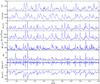 |
Fig. 1 Time series of CH, V, B, BV, AE, Ap, ΔDst, and Dst, from top to bottom respectively. |
The aim of this paper is to
-
1.
perform a systematic analysis of the relationships between CHcharacteristics, basic HSS/CIR parameters, and the mostrelevant geomagnetic indices for periods of low CME activity;
-
2.
study how the magnetospheric/ionospheric current systems (ring current and polar electrojets) behave when influenced by CIRs;
-
3.
check if and how the evolution of the background solar wind from 2005 to 2006 affected the correlations between CH, CIR, and geomagnetic parameters.
In Sect. 2 we present the data set. Time series of solar wind speed, V, magnetic field, B, and their combinations BV and BV2, along with the time series of geomagnetic indices Dst, Ap, and AE are described in Sect. 3. The correlations between CH characteristics, solar wind parameters, and geomagnetic indices are analyzed in Sect. 4. In Sect. 5 the results obtained for 2006 are compared with those obtained in Paper I for 2005. Finally, the results are discussed, and conclusions are drawn in Sect. 6.
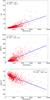 |
Fig. 2 Correlations BV–Ap, BV–AE and BV–Dst. The linear least-squares fit parameters, the correlation coefficient R, and the time lag Δt are shown in the insets. |
2. Data
In Paper I we focused on the period DOY = 25–125 of 2005. Here we analyze CIR-related geomagnetic activity during the period DOY = 60–261 of 2006, which was chosen because for this interval the GOES-12/SXI soft X-ray CH image product was available. In this period, we identified four intervals that were affected by the CME activity (DOY = 124–126, 191–192, 231–232, and 242–247), and consequently, we excluded them from the analysis. As in Paper I, the analysis is performed on the 6-h (1/4 day) data resolution.
For V and B we used the solar wind data measured by Solar Wind Electron Proton and Alpha Monitor (SWEPAM; McComas et al. 1998) and the magnetometer instrument (MAG; Smith et al. 1998) onboard the Advanced Composition Explorer (ACE; Stone et al. 1998). In particular, we used the merged hourly-averaged level-2 ACE data available at http://www.srl.caltech.edu/ACE/ASC/level2/.
Solar coronal hole fractional areas, CH (for details see Vršnak et al. 2007a), were determined from soft X-ray images acquired by the Soft X-ray Imager (SXI; Hill et al. 2005; Pizzo et al. 2005) onboard the GOES-12 spacecraft. The SXI coronal hole image product (level-2 files; see http://sxi.ngdc.noaa.gov/) was used to estimate CH for the central-meridian slice of the solar disk, which extends from the central meridian distance − 10° to + 10° (for details see Vršnak et al. 2007a).
We obtained the planetary geomagnetic activity index Ap, which measures the mid-latitude geomagnetic activity from http://wdc.kugi.kyoto-u.ac.jp/cgi-bin/kp-cgi. The storm-time disturbance index Dst, representing the longitudinally averaged magnetic field disturbance at the dipole equator on the Earth’s surface, is available at http://swdcwww.kugi.kyoto-u.ac.jp/dstdir/. For more details about these two indices see Verbanac et al. (2011). The auroral electrojet index AE, representing a quantitative global measure of the auroral zone magnetic activity (substorm activity), was obtained from http://wdc.kugi.kyoto-u.ac.jp/dstae/index.html. For more details about this index see Prolss (2004).
3. Time series
Time series of the analyzed parameters are shown in Fig. 1, where besides the CH fractional area CH, solar wind parameters B and V, and the geomagnetic indices Dst, Ap, and AE, we also present the products BV and BV2, as well as the change rate ΔDst, which represents the difference between the two successive Dst values. Note that the data of 2006 were also employed by different authors to study the effects of HSSs on the thermospheric density, thermospheric compositions, and the ionospheric total electron content (e.g., Thayer et al. 2008; Crowley et al. 2008; Lei et al. 2008c).
In the studied period, large equatorial coronal holes passed across the central meridian 21 times, resulting in 21 HSS/CIR structures at 1 AU. The HSSs are clearly seen in Fig. 1 as intervals of high velocity accompanied by a weak magnetic field. On the other hand, there is always a compression of the density and magnetic field (CIR) at the frontal side of HSS, which is caused by the interaction of the fast wind stream with the slow upstream wind. Typical peak values of V and B are 500–700 km s-1 and 10–15 nT, respectively.
Comparing the time series of geomagnetic indices in Fig. 1, one finds that the Ap and AE peaks are contemporaneous, and both occur during the decreasing phase of Dst (see also Fig. 2 of Verbanac et al. 2011). The Ap, AE, ΔDst peaks are in phase with BV. This behavior is consistent with the results presented in Paper I.
The time-profile of the AE index shows fluctuations that reflect the high temporal variability of the magnetic activity at high latitudes. The rise to the maximum activity is steep, which is followed by a relatively long decay. The Dst index shows a similar overall profile – a fairly sharp decrease is followed by a gradual increase. On the other hand, gradual decay is not as well pronounced in the Ap index, i.e., the decrease after the peak value is quite fast. The Ap time profiles are very similar to the ΔDst time-profiles.
The prolonged periods of AE activity, the so-called HILDCAA events (Tsurutani et al. 2006), can be noticed around DOY = 80 and 160. These events are associated with enhanced convection, driven by Alfvénic fluctuations within the HSSs. This effect provides an additional energy injection into the ring current, seen as a prolonged Dst depression, i.e., a slower and more noisy rise to the pre-storm state.
Linear least-squares fit coefficients a and b, correlation coefficient R, and the time lags Δt, describing the relationships between solar wind parameters and geomagnetic indices.
As seen in Fig. 1, most of the Dst decreases in the range between –30 nT and –50 nT, so they belong to weak geomagnetic disturbances (see, e.g., Gonzalez et al. 1994). Two moderate storms occurred in the studied period (Dst decrease between –50 nT and –100 nT), around DOY = 95 and 104. The strongest Dst decrease (–90 nT; DOY = 104) and the strongest increase of Ap (80 nT) is associated with the highest values of B (19 nT) and BV (10-2 V m-1). Note that this storm was not associated with the highest value of AE, which occurred on DOY = 231.75 (AE = 1067 nT). The latter indicates that the amount of energy injected into the ring current and into the polar ionosphere is not always in constant proportion, as noticed by Gonzalez et al. (1994). Note also that Dst decreases were not exceptionally high in days that we identified as being influenced by interplanetary CMEs. Only the CME that arrived on DOY = 231 caused a moderate storm (Dst = −64 nT), which was on the other hand associated with the strongest AE event in the analyzed period.
4. Cross-correlations
Below we investigate the relationship between the coronal hole characteristics, solar wind parameters, and geomagnetic indices by applying the cross-correlation analysis. In particular, we analyze how CH, V, and B are related to Ap, Dst, and AE. Furthermore, we include the combined solar wind parameters BV and BV2 because they turned out to be more important than V and B themselves (see Verbanac et al. 2011, and references therein).
Linear least-squares fit coefficients a and b, correlation coefficient R, and the time lags Δt, describing the relationships Dst(CH), AE(CH), Ap(CH), V(CH), and B(CH).
Linear least-squares fit coefficients a and b, correlation coefficient R, and the time lags Δt, describing the relationships between geomagnetic indices.
All cross-correlation functions are derived up to a time lag of ± 10 days with a step of six hours (the applied data resolution). A negative lag between two quantities, e.g., V and Ap, hereafter denoted as the V–Ap correlation, means that V is delayed with respect to Ap.
The results of the analysis are summarized in Table 1, where the linear least-squares fit parameters a and b, the correlation coefficient R, and the corresponding time lags Δt are presented. Besides the results for 2006, we also present the analogous values for 2005, to facilitate a comparison of the two periods, which are characterized by quite different background solar wind characteristics (see next section). The results for 2005 are mainly based on the analysis by Verbanac et al. (2011), supplemented by the AE index, and when necessary, re-formulated to be compatible with the presentation applied in this paper.
A given “X–Y” correlation corresponds to the linear form Y(t) = aX(t∗) + b, where X(t∗) represents the value of X that occurred Δt days before the actual value of Y, i.e., t∗ is the “retarded time”, t∗ = t − Δt. In Table 1 the time lags Δt are expressed in days.
Generally, all three geomagnetic indices are well correlated to the solar wind parameters V, B and their combinations. The best correlations are found for Ap index, then follows AE, whereas Dst shows somewhat weaker correlations. All geomagnetic indices are tightly correlated with BV2 and BV. The strongest Ap correlations may be related to the fact that Ap is affected by both polar and equatorial effects.
In Fig. 2 we present the scatter plots for the dependencies BV–Ap, BV–AE, and BV–Dst, where the highest-correlation time lag is applied. The data distribution in the graphs shows that there is an upper limit on both Ap and AE that is dependent on BV. This means that high values of these indices cannot be reached at low values of BV. On the other hand, a high value of BV does not imply large Ap and AE because there are data-points at Ap ≈ 0 and AE ≈ 0 even at high values of BV. Such a pattern was found for Ap in 2005 by Verbanac et al. (2011), where the upper limit on Ap attains practically the same values as here.
The triangular shape of the scatter plot found for Ap and AE is not present in the case of Dst. On the other hand, note that Dst does not achieve negative values if BV is below ≈ 1000 nT km s-1 corresponding to 1 mV m-1. In Paper I, this limit was found to be somewhat lower, BV ≈ 0.5 mV m-1.
Finally, we relate the geomagnetic indices directly to coronal holes because this might be used for forecasting purposes (Vršnak et al. 2007a; Verbanac et al. 2011). The outcome of the cross-correlation analysis along with results for 2005 are presented in Table 2. Both Ap and AE index are almost equally well correlated to CH, considerably better than Dst, especially in 2005. As expected, all of these correlations are lower than those obtained between geomagnetic indices and solar wind parameters.
5. Comparison with results for 2005
Inspecting Table 1 one finds that results for 2006 are similar to those for 2005, although the background solar wind speed and magnetic field decreased significantly between the two analyzed intervals. In 2005 the background value of V ranged around ≈350 km s-1 and in 2006 it decreased to ≈ 300 km s-1. At the same time the background B decreased from ≈3 nT to ≈2.5 nT.
Generally, correlation coefficients are higher in 2006. The time lags are almost always the same, the difference never exceeding 0.25 days, which corresponds to the applied time resolution. Furthermore, for both years, the highest correlation coefficients are found between geomagnetic indices and the products BV2, and BV. Generally, all three indices are better correlated with V than with B, except for Ap in 2006. On the other hand, ΔDst is correlated much better to B than to V in both years.
The general pattern, common to both years, is that the best correlations are obtained for Ap. Correlations for AE are somewhat weaker, whereas Dst shows the weakest correlation coefficients. For ΔDst, the correlation coefficients are even lower, and again they are somewhat higher in 2006. ΔDst peaks are in phase with BV and BV2 in both years.
In both years Ap and AE are better correlated with CH than Dst is. The difference is more prominent in 2005, when the correlations CH–Ap and CH–AE are considerably higher than in 2006. The same also holds for the CH–V and CH–B correlations.
All three considered geomagnetic indices exhibit a strong correlation with each other in both years as seen in Table 3. We note that the correlations are somewhat stronger in 2005, whereas the time delays are the same. The strongest correlation is found between Ap and AE (R = 0.8), without any time lag. Dst is almost equally well anti-correlated with both Ap and AE, Dst being delayed after Ap and AE for 0.25 days. This is consistent with the fact that Ap and AE peaks are contemporaneous with ΔDst. Moreover, the Ap–ΔDst and AE–ΔDst correlations are almost equal.
6. Discussion and conclusions
We studied the relationship between solar wind parameters, fractional coronal hole areas, and geomagnetic indices for 2006, DOY = 60–261. Furthermore, we compared the obtained results with the results for 2005 presented in Paper I. Both considered time-intervals cover the period of low CME activity, enabling us to investigate the magnetospheric activity caused solely by CIRs. We summarize our main results as follows:
-
1.
Results obtained for 2006 are similar to those obtained for2005: correlation coefficients for the studied relationships aresomewhat higher in 2006, whereas the time lags are mostlyidentical.
-
2.
All three considered geomagnetic indices, Ap, Dst and AE, are better correlated with BV2 and BV than with B and V; Ap and AE are better correlated with the solar wind parameters than Dst in both years.
-
3.
The strongest correlations without time lags are found between Ap and the solar wind parameters for both considered periods.
-
4.
Ap and AE are better correlated with CH than Dst for both considered periods;
-
5.
All three geomagnetic indices are tightly correlated to each other. The correlation coefficients are somewhat higher in 2005. The strongest correlation is found between geomagnetic indices Ap and AE (R > 0.8), without a time lag. Dst is almost equally well anti-correlated with both Ap and AE (R > 0.7), Dst being delayed after Ap and AE for 0.25 days; ΔDst peaks are in phase with BV and BV2 as well as with Ap and AE, in both years.
-
6.
The HSS/CIR-driven storms that occurred within the studied period are mostly weak (Dst between –50 nT and –30 nT) and only two of them are moderate (Dst –90 nT and –70 nT). This is in agreement with the fact that CIRs interaction with the Earth’s magnetosphere produces only weak to moderate intensity magnetic storms (Tsurutani et al. 2006).
-
7.
The recovery phases of observed storms lasted from a few days to a week and were associated with prolonged magnetic activity as monitored by the AE index. The observed AE fluctuations without large Dst variations may be interpreted as a substorm activity without appearance of significant storm activity.
We note that similar results for both years are obtained although the background solar wind speed and magnetic field decreased significantly between the two analyzed intervals. Thus, the performed analysis provides reliable relationships between CH properties, HSS/CIR parameters, and geomagnetic indices, which can be used in forecasting the geomagnetic activity in periods of low CME activity.
Furthermore, in this study we confirmed the results presented in Paper I, namely that combinations of solar wind parameters BV2 and BV play an essential role in the process of energy transfer from the solar wind to the magnetosphere. The physical mechanism behind the dominant correlation of all studied geomagnetic indices to BV and BV2 is as follows: the primary driver of geomagnetic disturbances is a strong convection electric field, BV, which is associated with the passage of the southward-directed interplanetary magnetic field Bs, which passes over the Earth for a sufficiently long time. This agrees with findings from Tsurutani et al. (1992), who demonstrated that high Bs rather than high V is the dominant part of the geoeffective electric field.
Note that in several previous studies a similar cross-correlation analysis was performed on longer time-scales, employing yearly averages of the studied quantities. For instance, Feynman (1980) reported that during cycle 20 Dst index has a weaker dependence on velocity than do the mid-latitude range aa index, i.e., that Dst varied as BV while aa varied as BV2.
Svalgaard & Cliver (2005) and Svalgaard & Cliver (2007) reported similar dependencies on even longer time intervals (1870–2005). They found that the IDV index (related to Dst) is highly correlated with the strength of the interplanetary magnetic field (R = 0.86) and almost unaffected by the solar wind speed (R = 0.1). On the other hand, they showed that the IHV index (related to Ap) is highly correlated with BV2.
In resolving the reason why our analysis has a somewhat different outcome, we have to take into account that when analyzing the whole cycle(s), contributions to the geomagnetic activity from both CMEs and HSSs are included. Because different magnetospheric current systems may respond differently to the HSS-related and the CME-related solar wind disturbances, the statistical results are likely to be somewhat different if HSS-related activity is analyzed separately.
Furthermore, when using annual averages, the peak values are smoothed out, whereas they were kept in our analysis. This means that our correlations are different because the ranges covered by the correlations are different. The velocity range in our study for instance is two and more than three times greater than in study of Svalgaard & Cliver (2007) and Feynman (1980), respectively. The IMF range in our study is about three times larger than in the mentioned studies, and the BV range in our study is about 30 times larger than the BV range covered by Feynman (1980).
Finally, we note that the records of middle latitude magnetometers contain contributions both from substorms currents (as quantified by AE) and ring current (as quantified by Dst), resulting in strong Ap–AE and Ap–Dst correlations (R = 0.81 and R = 0.7, respectively). The weaker Dst correlations are owing to the long-lasting recovery phase seen in Dst, which is not as prominent in AE and Ap time series. When the recovery is “removed” (by considering ΔDst), the Ap–ΔDst and AE–ΔDst correlations become similar.
The strong Dst–AE anti-correlation may be attributed to the storm/substorm coupling mechanism. Namely, the performed analysis shows that HSSs/CIRs cause weak to moderate storm activity, on average appearing six hours after the substorm activity. For low storm levels, the Dst and AE amplitudes
are practically proportional (Akasofu 19981). On the other hand, according to Saba et al. (1994) and Gonzalez et al. (1994), for intense storms (not present in our analysis) the AE values tend to saturate at about 1000 nT, suggesting storm/substorm decoupling.
The largest substorm that occurred within the studied period (AE = 1070 nT) was not accompanied with the strongest Dst, i.e., it caused only a moderate storm of Dst = −60 nT. This may be understood by recalling that the substorm expansive phase reflects an injection of energy in a way that may not be favorable for storage in the ring current. For instance, if the injection happens too far behind the Earth, the injected particles will be unable to contribute to the ring current. Furthermore, if the convection electric field is very high, the injected particles will most likely convect to the dayside magnetopause and will again not contribute to setting up the ring current.
In this respect, we also note that for the largest storm in the considered period (Dst = −90 nT), the AE index was lower (AE = 730 nT) than for the most intense substorm. It is possible that during this period, the auroral oval became somewhat lower in latitude, thus the AE observatories did not measure the electrojet perturbations at their peak in latitude, i.e., the strength of substorm activity might have been underestimated.
Acknowledgments
The research leading to these results has received funding from the European Commission’s Seventh Framework Programme (FP7/2007-2013) under the grant agreement No. 218816 (SOTERIA project, www.soteria-space.eu).
References
- Akasofu, S. I. 1981, J. Geophys. Res., 86, 4820 [NASA ADS] [CrossRef] [Google Scholar]
- Crowley, G., Reynolds, A., Thayer, J. P., et al. 2008, Geophys. Res. Lett., 35, L21106 [NASA ADS] [CrossRef] [Google Scholar]
- Feynman, J. 1980, Geophys. Res. Lett., 7, 971 [NASA ADS] [CrossRef] [Google Scholar]
- Gonzalez, W. D., Joselyn, J., Kamide, Y., et al. 1994, J. Geophys. Res., 99, 5771 [Google Scholar]
- Hill, S. M., Pizzo, V. J., Balch, C. C., et al. 2005, Sol. Phys., 226, 255 [Google Scholar]
- Lei, J., Thayer, J. P., Forbes, J. M., & Sutton, E. K. 2008a, AGU Fall Meeting Abstracts, A3 [Google Scholar]
- Lei, J., Thayer, J. P., Forbes, J. M., Sutton, E. K., & Nerem, R. S. 2008b, Geophys. Res. Lett., 35, 10109 [Google Scholar]
- Lei, J., Thayer, J. P., Forbes, J. M., et al. 2008c, Geophys. Res. Lett., 35, 19105 [NASA ADS] [CrossRef] [Google Scholar]
- McComas, D., Bame, S. J., Barker, P., et al. 1998, Space Sci. Rev., 86, 563 [NASA ADS] [CrossRef] [Google Scholar]
- Miyoshi, Y., Morioka, A., Kataoka, R., Kasahara, Y., & Mukai, T. 2007, J. Geophys. Res. (Space Physics), 112, 5210 [NASA ADS] [CrossRef] [Google Scholar]
- Nolte, J. T., Krieger, A. S., Timothy, A. F., et al. 1976, Sol. Phys., 46, 303 [NASA ADS] [CrossRef] [Google Scholar]
- Pizzo, V. J., Hill, S. M., Balch, C. C., et al. 2005, Sol. Phys., 226, 283 [NASA ADS] [CrossRef] [Google Scholar]
- Prolss, G. 2004, Physics of the Earth’s Space Environment (Berlin Heidelberg: Springer-Verlag) [Google Scholar]
- Saba, M. M. F., Gonzalez, W. D., & de Gonzalez, A. L. C. 1994, in Solar-Terrestrial Energy Program, ed. D. N. Baker, V. O. Papitashvili, & M. J. Teague, 435 [Google Scholar]
- Smith, C. W., L’Heureux, J., Ness, N. F., et al. 1998, Space Sci. Rev., 86, 613 [NASA ADS] [CrossRef] [Google Scholar]
- Stone, E. C., Frandsen, A. M., Mewaldt, R. A., et al. 1998, Space Sci. Rev., 86, 1 [Google Scholar]
- Svalgaard, L., & Cliver, E. W. 2005, J. Geophys. Res., 110 (A9), 12103 [Google Scholar]
- Svalgaard, L., & Cliver, E. W. 2007, J. Geophys. Res. (Space Physics), 112, A10111 [Google Scholar]
- Thayer, J. P., Lei, J., Forbes, J. M., Sutton, E. K., & Nerem, R. S. 2008, J. Geophys. Res. (Space Physics), 113, 6307 [Google Scholar]
- Tsurutani, B. T., Gonzalez, W. D., Tang, F., & Te Lee, Y. 1992, Geophys. Res. Lett., 19, 73 [NASA ADS] [CrossRef] [Google Scholar]
- Tsurutani, B. T., McPherron, R. L., Gonzalez, W. D., et al. 2006, J. Geophys. Res., 111, 1 [Google Scholar]
- Verbanac, G., Vršnak, B., Temmer, M., & Veronig, A. 2011, A&A, 526, A20 [Google Scholar]
- Vršnak, B., Temmer, M., & Veronig, A. 2007a, Sol. Phys., 240, 315 [Google Scholar]
- Vršnak, B., Temmer, M., & Veronig, A. 2007b, Sol. Phys., 240, 331 [Google Scholar]
All Tables
Linear least-squares fit coefficients a and b, correlation coefficient R, and the time lags Δt, describing the relationships between solar wind parameters and geomagnetic indices.
Linear least-squares fit coefficients a and b, correlation coefficient R, and the time lags Δt, describing the relationships Dst(CH), AE(CH), Ap(CH), V(CH), and B(CH).
Linear least-squares fit coefficients a and b, correlation coefficient R, and the time lags Δt, describing the relationships between geomagnetic indices.
All Figures
|
Fig. 1 Time series of CH, V, B, BV, AE, Ap, ΔDst, and Dst, from top to bottom respectively. |
| In the text | |
|
Fig. 2 Correlations BV–Ap, BV–AE and BV–Dst. The linear least-squares fit parameters, the correlation coefficient R, and the time lag Δt are shown in the insets. |
| In the text | |
Current usage metrics show cumulative count of Article Views (full-text article views including HTML views, PDF and ePub downloads, according to the available data) and Abstracts Views on Vision4Press platform.
Data correspond to usage on the plateform after 2015. The current usage metrics is available 48-96 hours after online publication and is updated daily on week days.
Initial download of the metrics may take a while.