| Issue |
A&A
Volume 532, August 2011
|
|
|---|---|---|
| Article Number | A41 | |
| Number of page(s) | 11 | |
| Section | Astrophysical processes | |
| DOI | https://doi.org/10.1051/0004-6361/201116702 | |
| Published online | 20 July 2011 | |
Spinning up black holes with super-critical accretion flows
1
Nicolaus Copernicus Astronomical Center, Polish Academy of Sciences, Bartycka 18, 00-716 Warszawa, Poland
e-mail: This email address is being protected from spambots. You need JavaScript enabled to view it.
; This email address is being protected from spambots. You need JavaScript enabled to view it.
; This email address is being protected from spambots. You need JavaScript enabled to view it.
2 Astronomical Institute, Academy of Sciences of the Czech Republic, Boční II 1401/1a, 141-31 Praha 4, Czech Republic
e-mail: This email address is being protected from spambots. You need JavaScript enabled to view it.
3
Department of Physics, Göteborg University, 412-96 Göteborg, Sweden
e-mail: This email address is being protected from spambots. You need JavaScript enabled to view it.
4
Department of Physics, Silesian University at Opava, Bezručovo náměstí 1150/13, 74601 Opava, Czech Republic
5
Institut d’Astrophysique de Paris, UMR 7095 CNRS, UPMC Univ. Paris 06, 98bis Bd Arago, 75014 Paris, France
e-mail: This email address is being protected from spambots. You need JavaScript enabled to view it.
6
Jagiellonian University Observatory, ul. Orla 171, 30-244 Kraków, Poland
7
Department of Physics and Astronomy, Johns Hopkins University, 3400 N. Charles Street Baltimore, MD 21218, USA
e-mail: This email address is being protected from spambots. You need JavaScript enabled to view it.
Received: 11 February 2011
Accepted: 24 May 2011
Abstract
We study the process of spinning up black holes by accretion from slim disks for a wide range of accretion rates. We show that for super-Eddington accretion rates and low values of the viscosity parameter α ( ≲ 0.01) the limiting value of the dimensionless spin parameter a∗ can reach values higher than a∗ = 0.9978 inferred by Thorne in his seminal study. For Ṁ = 10 ṀEdd and α = 0.01, spin equilibrium is reached at a∗ = 0.9994. We show that the equilibrium spin value depends strongly on the assumed value of α. We also prove that for high accretion rates the impact of captured radiation on spin evolution is negligible.
Key words: black hole physics / accretion, accretion disks
© ESO, 2011
1. Introduction
Astrophysical black holes (BHs) are very simple objects – they can be described by just two parameters: mass M and angular momentum J (usually described by the dimensionless spin parameter a∗ ≡ a/M = J/M2). In isolation, BHs conserve the birth values of these parameters but are often surrounded by accretion disks and experience both mass and angular momentum change, e.g., in close binaries or in active galactic nuclei. Accretion of matter always increases the BH’s irreducible mass and may change its angular momentum. The sign of this change and its value depend on the (relative) sign of accreted angular momentum and the balance between the accretion of matter and various processes extracting the BH’s rotational energy and angular momentum.
The question about the maximal possible spin of an object represented by the Kerr solution of the Einstein equation is of fundamental and practical (observational) interest. First, a spin a∗ > 1 corresponds to a naked singularity and not to a black hole. According to the Penrose cosmic censorship conjecture, naked singularities cannot form through actual physical processes, i.e. singularities in the Universe (except for the initial one in the Big Bang) are always surrounded by event horizons (Wald 1984). This hypothesis has yet to be proven.
In any case, the “third law” of BH thermodynamics (Bardeen et al. 1973) asserts that a BH cannot be spun-up in a finite time to the extreme spin value a∗ = 1. Determining the maximum value of BH spin is also of practical interest because the radiative efficiency of disk accretion depends on the BH’s spin value. For example, for the “canonical” value a∗ = 0.9978 (see below) it is about η ≈ 32%, while for a∗ → 1 one has η → 42%. Bañados et al. (2009) showed that the energy of the center-of-mass collision of two particles colliding arbitrary close to the BH horizon, grows to infinity1 when a∗ → 1.
A definitive study of the BH spin evolution will only be possible when reliable, non-stationary models of accretion disks and jet emission mechanisms are established. For now, one has to use simplified analytical or numerical models.
Thorne (1974) used the model of a radiatively efficient, geometrically thin accretion disk (Novikov & Thorne 1973) to evaluate BH spin evolution taking into account the decelerating impact of disk-emitted photons. The maximum value obtained to date a∗ = 0.9978, has been regarded as the canonical value for the maximal BH spin. In this work, we generalize Thorne’s approach, using hydrodynamical models of advective, α-viscosity, optically thick accretion disks (“slim disks”) to calculate maximum BH spin values for a large range of accretion rates. Following Thorne (1974), we assume that accretion of matter and radiation captured by the BH are the only mechanisms affecting its rotation. Thus, we neglect any impact of large-scale magnetic fields (a discussion of the applicability of slim disks is presented in Sect. 6). We show that for sufficiently high accretion rates the limiting BH spin differs from the canonical value.
We begin with a short discussion of previous work devoted to the evolution of BH spin. In Sect. 2, we present formulae for a general tetrad (an orthonormal set of four vector fields, one timelike and three spacelike) of an observer comoving with the accreting gas along the arbitrary photosphere surface. In Sect. 3, we give basic equations describing the BH spin evolution. Section 4 describes the model of slim accretion disks. In Sect. 5, we present and discuss the terminal spin values for all the models considered. Finally, in Sect. 6 we summarize our results.
1.1. Previous studies
A number of authors have studied the BH spin evolution resulting from disk accretion. Bardeen (1970) initiated this field of research by solving equations describing the BH spin evolution for accretion from the marginally stable orbit. Neglecting the effects of radiation, he proved that this accretion could spin-up the BH arbitrarily close to a∗ = 1. Once the classical models of accretion disks were formulated (Shakura & Sunyaev 1973; Novikov & Thorne 1973), it was possible to account properly for the decelerating impact of radiation (frame dragging makes counter-rotating photons more likely to be captured by the BH). As mentioned above, Thorne (1974) performed this study and obtained for an isotropically emitting thin disk the terminal BH spin a∗ = 0.9978, independently of the accretion rate. The original study by Thorne was followed by many papers, some of which are briefly mentioned below.
The first to challenge the universality of Thorne’s limit were Abramowicz & Lasota (1980), who showed that geometrically thick accretion disks may spin up BHs to terminal spin values much closer to unity than the canonical a∗ = 0.9978. Their simple argument was based on models by Kozlowski et al. (1978), who showed that for high accretion rates the inner edge of a disk may be located inside the marginally stable orbit, and in fact, with increasing accretion rate, arbitrarily close to the marginally bound orbit. However, this conclusion assumed implicitly a low viscosity parameter α, whereas for high viscosities the situation is more complicated (see Abramowicz et al. 2010, and references therein).
Moderski et al. (1998) assessed the impact of possible interaction between the disk magnetic field and the BH through the Blandford-Znajek process. They showed that the terminal spin value may be decreased to any, arbitrarily small value, if the disk magnetic field is strong enough. Given the current lack of self-consistent and reliable models of accretion disks with large-scale magnetic fields, a more detailed study cannot be performed. The situation may be further complicated by energy extraction from the inner parts of accretion disks and the magnetic transport of angular momentum (see Livio et al.1999; Ghosh & Abramowicz1997; and compare with McKinney & Narayan2007).
Popham & Gammie (1998) studied the spinning-up of BHs by optically thin advection dominated accretion flows (ADAFs). They neglected the contribution of radiation to BH spin because such accretion disks are radiatively inefficient. They found that the terminal value of BH spin is very sensitive to the assumed value of the viscosity parameter α and may vary between 0.8 and 1.0. Gammie et al. (2004), in addition to comprehensively summarizing the different ways of spinning up supermassive BHs, presented results based on a set of relativistic magnetohydrodynamical (GRMHD) simulations (with no radiation included) obtaining a terminal spin of a∗ = 0.93.
The cosmological evolution of the spins of supermassive BHs caused by hierarchical mergers and thin-disk accretion episodes has been intensively studied. Although Volonteri et al. (2005) arrived at the conclusion that accretion tends to spin-up BHs close to a∗ = 1, as opposed to mergers, which, on the average, do not influence the spin, subsequent studies by, e.g., Volonteri et al. (2007), King et al. (2008) and Berti & Volonteri (2008) showed that the situation is more complex, the final spin values depending on the details of the history of the accretion events (see also Fanidakis et al. 2011).
Belczynski et al. (2008) applied population synthesis methods to estimate BH spins in coalescing compact star binaries. Basing their calculations on results of radiation-hydrodynamic simulations of thick accretion disks by Ohsuga (2007), they neglected the impact of radiation on BH spin and assumed that gas is transferred from the innermost stable orbit conserving Keplerian angular momentum. They showed that the spin parameter a∗ resulting from the coalescence is not expected to exceed 0.5 for those BHs that are not spun-up during the star collapse.
Li et al. (2005) included the radiation returning to the disk in the thin-disk model of Novikov & Thorne and calculated the spin-up limit for the BH assuming radiation crossing the equatorial plane inside the marginally stable orbit is advected onto the BH. Their result (a∗ = 0.9983) differs slightly from Thorne’s result, thus showing that returning radiation has only a slight impact on the process of spinning-up BHs. In our study, we use advective, optically thick solutions of accretion disks and account for photons captured by the BH in detail. However, we neglect the impact on the disk structure of the returning radiation.
2. The tetrad
We base this work on slim accretion disks, which are not razor-thin and have an angular momentum profile that is not Keplerian (for details about the assumptions made and the disk appearance see Sect. 4). Therefore, photons are not emitted from matter in Keplerian orbits in the equatorial plane and the classical expressions for photon momenta (e.g., Misner et al. 1973) cannot be applied. To properly describe the momentum components of emitted photons, we need a tetrad for the comoving observer instantaneously located at the disk photosphere. Below we give the explicit expression for the components of such a tetrad assuming time and axis symmetries. A detailed derivation is given in Appendix A.
We choose the following comoving tetrad ![Mathematical equation: \begin{equation} \label{tetrad} e^i_{(\alpha)} = \left[u^i,N^i,\kappa^i,S^i\right], \end{equation}](/articles/aa/full_html/2011/08/aa16702-11/aa16702-11-eq24.png) (1)where ui is the four-velocity of matter, Ni is a unit vector in the [r,θ] plane that is orthogonal to the photosphere, κi is a unit vector in the [t,φ] plane that is orthogonal to ui, and Si is a unit vector orthogonal to ui, Ni, and κi.
(1)where ui is the four-velocity of matter, Ni is a unit vector in the [r,θ] plane that is orthogonal to the photosphere, κi is a unit vector in the [t,φ] plane that is orthogonal to ui, and Si is a unit vector orthogonal to ui, Ni, and κi.
The tetrad components are given by ![Mathematical equation: \begin{eqnarray} N^r &=& \der{\theta_*}r \left(-g_{\theta\theta}\right)^{-1/2} \left[1+\frac{g_{rr}}{g_{\theta\theta}}\left(\der{\theta_*}r\right)^2\right]^{-1/2},\\[1.5mm] N^\theta &=& \left(-g_{\theta\theta}\right)^{-1/2} \left[1+\frac{g_{rr}}{g_{\theta\theta}} \left(\der{\theta_*}r\right)^2\right]^{-1/2},\\[1.5mm] u^i &=& \frac{\eta^i+\Omega\xi^i+vS^i_*}{\sqrt{g_{tt}+\Omega g_{\phi\phi}(\Omega-2\omega)-v^2}},\\[1.5mm] \kappa^i &=& \frac{\left(l\eta^i+\xi^i\right)}{\left[-g_{\phi\phi}(1-\Omega l)(1-\omega l)\right]^{1/2}},\\[1.5mm] S^i &=& \left(1+\tilde A^2v^2\right)^{-1/2}\left(\tilde A vu^i+S^i_*\right), \end{eqnarray}](/articles/aa/full_html/2011/08/aa16702-11/aa16702-11-eq31.png) where θ = θ∗(r) defines the location of the photosphere, ηi and ξi are the Killing vectors, l = uφ/ut, Ω = uφ/ut, ω is the frequency of frame-dragging, and the expressions for v and
where θ = θ∗(r) defines the location of the photosphere, ηi and ξi are the Killing vectors, l = uφ/ut, Ω = uφ/ut, ω is the frequency of frame-dragging, and the expressions for v and  are given in Eqs. (A.10) and (A.4), respectively.
3. Spin evolution
3.1. Basic equations
The equations describing the evolution of dimensionless BH spin a∗ with respect to the BH energy M and the accreted rest-mass M0 are (Thorne 1974) ![Mathematical equation: \begin{eqnarray} \label{eq.spinevolution1} \der{a_*}{{\rm ln} M} &=& \der{J/M^2}{{\rm ln} M}=\frac 1M\frac{\dot M_0 u_{\phi}+\left(\der Jt\right)_{\rm rad}}{\dot M_0 u_{t}+\left(\der Mt\right)_{\rm rad}}-2a_*,\\[1.5mm] \label{eq.spinevolution2} \der M{M_0} &=& u_{t}+\left(\der Mt\right)_{\rm rad}/\dot M_0. \end{eqnarray}](/articles/aa/full_html/2011/08/aa16702-11/aa16702-11-eq41.png) The energy and angular momentum of BH increase due to the capture of photons according to the formulae
The energy and angular momentum of BH increase due to the capture of photons according to the formulae ![Mathematical equation: \begin{eqnarray} \label{e.dM} ({\rm d}M)_{\rm rad} &=& \int^{}_{\rm disk} T^{ik}\eta_k N_i{\rm d}S,\\[1.5mm] \label{e.dJ} ({\rm d}J)_{\rm rad} &=& \int^{}_{\rm disk} T^{ik}\xi_k N_i{\rm d}S, \end{eqnarray}](/articles/aa/full_html/2011/08/aa16702-11/aa16702-11-eq42.png) where ηk and ξk are the Killing vectors connected with time and axial symmetries, respectively, Tik is the stress-energy tensor of photons, which is taken to be non-zero only for photons crossing the BH horizon, and dS is the “volume element” in the hypersurface orthogonal to Ni, which is given by Eq. (B.8).
where ηk and ξk are the Killing vectors connected with time and axial symmetries, respectively, Tik is the stress-energy tensor of photons, which is taken to be non-zero only for photons crossing the BH horizon, and dS is the “volume element” in the hypersurface orthogonal to Ni, which is given by Eq. (B.8).
From Eqs. (9) and (10), it follows that ![Mathematical equation: \begin{eqnarray} \label{e.dMdt1} \left(\der Mt\right)_{\rm rad} &=& \int^{2\pi}_0\int_{r_{\rm in}}^{r_{\rm out}}T^{ik}\eta_k N_i {\rm d}\tilde S, \\[1.5mm] \label{e.dJdt1} \left(\der Jt\right)_{\rm rad} &=& \int^{2\pi}_0\int_{r_{\rm in}}^{r_{\rm out}}T^{ik}\xi_k N_i {\rm d}\tilde S, \end{eqnarray}](/articles/aa/full_html/2011/08/aa16702-11/aa16702-11-eq47.png) where
where  (13)
(13)
3.2. Stress energy tensor in the comoving frame
We select the tetrad given in Eq. (1) ![Mathematical equation: \begin{eqnarray} \label{e.comtetrad} e^i_{(0)} &=& u^i \qquad e^i_{(1)}=N^i\nonumber\\[1.5mm] e^i_{(2)} &=& \kappa^i \qquad e^i_{(3)}= S^i. \end{eqnarray}](/articles/aa/full_html/2011/08/aa16702-11/aa16702-11-eq49.png) (14)The disk properties, e.g., the emitted flux, are usually given in the comoving frame defined by Eq. (14). The stress tensor components in the two frames (Boyer-Lindquist and comoving) are related in the following way:
(14)The disk properties, e.g., the emitted flux, are usually given in the comoving frame defined by Eq. (14). The stress tensor components in the two frames (Boyer-Lindquist and comoving) are related in the following way:  (15)The stress tensor in the comoving frame is
  (16)where
  is the intensity of the emitted radiation,
  and
and  are the angles between the emission vector and the Ni and Si vectors, respectively, C is the capture function defined in Sect. 3.4, the factor 2 occurs because the disk emission comes from both sides of the disk, and π(α) = p(α)/p(0) are the normalized components of the photon four-momentum in the comoving frame. The last set of parameters are given by the relations (Thorne 1974)
 ![Mathematical equation: \begin{eqnarray} \pi^{(0)}&=&1,\nonumber\\[1.5mm] \pi^{(1)}&=&\cos \tilde a,\nonumber\\[1.5mm] \pi^{(2)}&=&\sin{\tilde a}\cos \tilde b,\nonumber\\[1.5mm] \pi^{(3)}&=&\sin{\tilde a}\sin \tilde b. \end{eqnarray}](/articles/aa/full_html/2011/08/aa16702-11/aa16702-11-eq58.png) (17)Equations (11) and (12) take the form
(17)Equations (11) and (12) take the form ![Mathematical equation: \begin{eqnarray} \label{e.dMdt2} \left(\der Mt\right)_{\rm rad} &=& \int^{}_{\rm disk} T^{(\alpha)(\beta)}e^{i}_{(\alpha)} e^{k}_{(\beta)}\eta_k N_i{\rm d}\tilde S, \\[1.5mm] \label{e.dJdt2} \left(\der Jt\right)_{\rm rad} &=& \int^{}_{\rm disk}T^{(\alpha)(\beta)}e^{i}_{(\alpha)}e^{k}_{(\beta)}\xi_k N_i{\rm d}\tilde S, \end{eqnarray}](/articles/aa/full_html/2011/08/aa16702-11/aa16702-11-eq59.png) where
where  is our local frame tetrad given by Eq. (14).
Taking into account the relations ![Mathematical equation: \begin{eqnarray} \pi^{(\alpha)} &=& \pi^je^{(\alpha)}_j,\nonumber\\[1.5mm] e^{(\alpha)}_je_{(\alpha)}^i &=& \delta_j^i, \end{eqnarray}](/articles/aa/full_html/2011/08/aa16702-11/aa16702-11-eq61.png) (20)we have
(20)we have ![Mathematical equation: \begin{eqnarray} \pi^{(\alpha)}e^{i}_{(\alpha)}N_i &=& \pi^{(\alpha)}\delta^{(1)}_{(\alpha)}=\pi^{(1)}=\cos \tilde a, \\[1.5mm] \pi^{(\beta)}e^{k}_{(\beta)}\eta_k &=& \pi^je^{(\beta)}_je^k_{(\beta)}\eta_k = \pi^j\delta_j^k\eta_k=\pi^k\eta_k=\pi_t, \\[1.5mm] \pi^{(\beta)}e^{k}_{(\beta)}\xi_k &=& \pi^je^{(\beta)}_je^k_{(\beta)}\xi_k= \pi^j\delta_j^k\xi_k=\pi^k\xi_k=\pi_\phi, \end{eqnarray}](/articles/aa/full_html/2011/08/aa16702-11/aa16702-11-eq62.png) where,
where, ![Mathematical equation: \begin{eqnarray} \pi_t &=& \pi^{(i)}e^t_{(i)} g_{tt} + \pi^{(i)}e^\phi_{(i)}g_{t\phi},\\[1.5mm] \pi_\phi &=& \pi^{(i)}e^t_{(i)} g_{t\phi} + \pi^{(i)}e^\phi_{(i)} g_{\phi\phi}. \end{eqnarray}](/articles/aa/full_html/2011/08/aa16702-11/aa16702-11-eq63.png) Therefore, Eqs. (18) and (19) may be finally expressed as
Therefore, Eqs. (18) and (19) may be finally expressed as ![Mathematical equation: \begin{eqnarray} \left(\der Mt\right)_{\rm rad} &=& 4\pi\int_{r_{\rm in}}^{r_{\rm out}} \int_0^{2\pi} \int_0^{\pi/2}I_0SC\pi_t\nonumber \\[1.5mm] &&\times\cos\tilde a\sin\tilde a\,{\rm d}\tilde a\,{\rm d}\tilde b \sqrt{\tilde g}\,{\rm d}r, \\[1.5mm] \left(\der Jt\right)_{\rm rad} &=& 4\pi\int_{r_{\rm in}}^{r_{\rm out}}\int_0^{2\pi} \int_0^{\pi/2} I_0SC\pi_\phi\nonumber\\[1.5mm] &&\times \cos\tilde a\sin\tilde a\,{\rm d}\tilde a\,{\rm d}\tilde b \sqrt{\tilde g}\,{\rm d}r, \end{eqnarray}](/articles/aa/full_html/2011/08/aa16702-11/aa16702-11-eq64.png) where
where  (28)
(28)
3.3. Emission
The intensity of local radiation may be identified with the flux emerging from the disk surface  (29)The angular emission factor S was taken by Thorne (1974) to be
 ![Mathematical equation: \begin{equation} S\left(\tilde a,\tilde b\right) = \left\{ \begin{array}{ll} 1/\pi & {\rm isotropic}\\[1.5mm] (3/7\pi)\left(1+2\cos\tilde a\right)& {\rm limb\,darkening}\\ \end{array}\right. \end{equation}](/articles/aa/full_html/2011/08/aa16702-11/aa16702-11-eq68.png) (30)for isotropic and limb-darkened cases, respectively. In this work, we assume that the radiation is emitted isotropically.
(30)for isotropic and limb-darkened cases, respectively. In this work, we assume that the radiation is emitted isotropically.
3.4. Capture function
The BH energy and angular momentum are affected only by photons crossing the BH horizon. Following Thorne (1974), we define the capture function C![Mathematical equation: \begin{equation} C = \left\{ \begin{array}{ll} 1& {\rm if\ the\ photon\ hits\ the\ BH,}\\[1.5mm] 0& {\rm in\ the\ opposite\ case.}\\ \end{array}\right. \end{equation}](/articles/aa/full_html/2011/08/aa16702-11/aa16702-11-eq69.png) (31)Herein, we calculate C in two ways. First, we use the original Thorne (1974) algorithm modified to account for emission out of the equatorial plane. For this purpose, we calculate the constants of motion, j and k, for a geodesic orbit of a photon using
(31)Herein, we calculate C in two ways. First, we use the original Thorne (1974) algorithm modified to account for emission out of the equatorial plane. For this purpose, we calculate the constants of motion, j and k, for a geodesic orbit of a photon using ![Mathematical equation: \begin{eqnarray} j &=& a_*^2+a_*\left(\pi_\phi/M\pi_t\right), \\[1.5mm] k &=& \frac1{\left(M\pi_t\right)^2}\left[\pi_\theta^2-\left(\pi_\phi+a_*M\pi_t \sin\theta_*\right)^2/\sin^2\theta_*\right] \end{eqnarray}](/articles/aa/full_html/2011/08/aa16702-11/aa16702-11-eq72.png) which replaces Thorne’s Eq. (A10). This approach does not take into account the effects of returning radiation, i.e., a photon hitting the disk surface is assumed to continue its motion. This treatment is inappropriate for optically thick disks – returning photons are most likely absorbed or advected towards the BH.
which replaces Thorne’s Eq. (A10). This approach does not take into account the effects of returning radiation, i.e., a photon hitting the disk surface is assumed to continue its motion. This treatment is inappropriate for optically thick disks – returning photons are most likely absorbed or advected towards the BH.
To assess the importance of this inconsistency, we adopt two additional algorithms for calculating C. Using photon equations of motion, we determine whether the photon hits the disk surface (Bursa 2006). We then make one of two assumptions, either the angular momentum and energy of all “returning” photons are advected onto the BH (C1), or all are re-emitted carrying away their original angular momentum and energy, and never hit the BH (C2). In this way, we establish two limiting cases allowing us to assess the impact of the returning radiation.
We note that for a fully consistent treatment of the returning radiation (as in Li et al. 2005, for geometrically thin disks) it is not enough to modify the capture function, but that finding a solution for the whole structure of a self-irradiated accretion disk is instead necessary. The latter has not yet been done for luminous and geometrically thick disks. We are currently working on implementing such a scheme and will study its impact on BH spin evolution in an upcoming paper.
4. Slim accretion disks
4.1. Equations
We now introduce slim disk equations. They were derived originally by Lasota (1994) and improved e.g., by Abramowicz et al. (1996) and Gammie & Popham (1998). Here, we follow Kato et al. (2008) and assume the polytropic equation of state when performing vertical integration. The formalism we use here was adopted from Sądowski et al. (2011).
In the structure equations, we assume that G = c = 1, and use expressions involving the BH spin given by ![Mathematical equation: \begin{eqnarray} \Delta &=& r^2 - 2Mr + a^2,\nonumber\\[1.5mm] A &=& r^4 + r^2a^2 + 2Mra^2,\nonumber\\[1.5mm] \cal C &=& 1 - 3r_*^{-1} + 2a_*r_*^{-3/2},\nonumber\\[1.5mm] \cal D &=& 1 - 2r_*^{-1}+2a_*^2r_*^{-2},\nonumber\\[1.5mm] \cal H &=& 1-4a_*r_*^{-3/2}+3a_*^{2}r_*^{-2}, \end{eqnarray}](/articles/aa/full_html/2011/08/aa16702-11/aa16702-11-eq76.png) (34)where a∗ = a/M and r∗ = r/M.
(34)where a∗ = a/M and r∗ = r/M.
We also define  (35)and a dimensionless accretion rate ṁ = Ṁ/ṀEdd, where ṀEdd = 16LEdd/c2 is the critical accretion rate corresponding approximately to the Eddington luminosity (LEdd = 1.25 × 1038 M/M⊙ erg/s) for a disk around a non-rotating black hole.
The equations describing slim disks written in the cylindrical coordinates are:
-
(i)
for mass conservation
 (36)where
  is the disk surface density,
while v denotes the gas velocity as measured by an observer
co-rotating with the fluid and is related to the
four-velocity ur by
is the disk surface density,
while v denotes the gas velocity as measured by an observer
co-rotating with the fluid and is related to the
four-velocity ur by  ;
; -
(ii)
for radial momentum conservation
 (37)where
  (38)and
Ω = uφ/ut
is the angular velocity with respect to a stationary observer,
(38)and
Ω = uφ/ut
is the angular velocity with respect to a stationary observer,  is the angular velocity with respect to an
inertial observer,
is the angular velocity with respect to an
inertial observer,  are the angular frequencies of the co-rotating
and counter-rotating Keplerian orbits,
are the angular frequencies of the co-rotating
and counter-rotating Keplerian orbits,  is the radius of gyration, and
  is the vertically integrated total pressure;
 -
(iii)
for angular momentum conservation
 (39)where
ℒ = uφ, ℒin is a constant,
and Γ is the Lorentz factor (Gammie & Popham
1998)
(39)where
ℒ = uφ, ℒin is a constant,
and Γ is the Lorentz factor (Gammie & Popham
1998)  (40)
(40) -
(iv)
for vertical equilibrium
 (41)
(41) -
(v)
for energy conservation
![Mathematical equation: \begin{eqnarray} \label{eq.qadv} Q^{\rm adv} &=& -\frac{\mdot}{2\pi R^2}\left(\eta_3\frac{P}\Sigma\derln{P}{R} - \left(1+\eta_3\right) \frac{P}\Sigma\derln\Sigma R\right.\nonumber\\[0.5mm] &&+\left. \eta_3\frac P\Sigma\derln{\eta_3}{R}+\Omega^2_\perp\eta_4\derln{\eta_4}{R}\right), \end{eqnarray}](/articles/aa/full_html/2011/08/aa16702-11/aa16702-11-eq100.png) (42)where the amount of heat advected
Qadv is
(42)where the amount of heat advected
Qadv is  (43)Assuming the polytropic index
N = 3, we have
(43)Assuming the polytropic index
N = 3, we have ![Mathematical equation: \begin{eqnarray} \eta_1 &=& \frac1{T_0^4}\int_0^HT^4\,{\rm d}z=128/315\, H,\nonumber\\[0.5mm] \eta_2 &=& \frac2{\Sigma T_0}\int_0^H\rho T\,{\rm d}z=40/45,\nonumber\\[0.5mm] \eta_3 &=& \frac1P\left(\frac1{5/3-1}\frac{k}\mu\frac{40}{45}\Sigma T_{\rm C} + \frac{256}{315}aT^4_{\rm C}H\right),\nonumber\\[0.5mm] \eta_4 &=& \frac1{\Sigma}\int_0^H\rho z^2\,{\rm d}z=1/18\, H^2. \end{eqnarray}](/articles/aa/full_html/2011/08/aa16702-11/aa16702-11-eq104.png) (44)
(44)
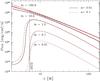 |
Fig. 1 Flux profiles for M = 10 M⊙ and a∗ = 0.0. |
4.2. Disk appearance
We now briefly describe the properties of slim disk solutions. For a more detailed discussion, we refer to e.g., Sądowski (2009), Abramowicz et al. (2010), and Bursa et al. (in prep.).
The radial profiles of the emitted flux for a non-rotating BH are presented in Fig. 1. For low accretion rates (ṁ ≪ 1), they almost coincide with the Novikov & Thorne solutions (the small departure is due to the angular momentum taken away by photons, an effect that is neglected in our slim disk scheme). When the accretion rate becomes high, advective cooling starts to play a significant role and the emission departs from that of the radiatively efficient solution. This departure is visible as early as for ṁ = 1 at which the emission extends significantly inside the marginally stable orbit. For super-critical accretion rates, the flux increases monotonically towards the BH horizon. Different colors in Fig. 1 denote solutions for different values of the viscosity parameter α. Although the solutions are very similar, one can see that the higher the value of α, the lower the accretion rate at which advection starts to modify the emission profile.
In Fig. 2, we plot disk thickness profiles (cosΘH = H/r) for a range of accretion rates and two values of α. For ṁ > 0.1, the inner region of the accretion disk is puffed up by the radiation pressure and the disk surface corresponds to the location where the radiation pressure force (which is proportional to the local flux of emitted radiation) is balanced by the vertical component of the gravity force. For the Eddington accretion rate (ṁ ≈ 1), the highest H/R ratio equals ~0.3 (cosΘH ≈ 0.3), while for the highest accretion rate considered (ṁ = 100) it reaches ~1.5 (cosΘH ≈ 0.83).
In the thin disk approximation, the accreting fluid has a Keplerian angular momentum. This condition is not satisfied for advective accretion disks with significant radial pressure gradients. In Fig. 3, we present angular momentum profiles for disks with different accretion rates, α = 0.01 (left) and α = 0.1 (right panel). It is clear that the higher the accretion rate, the larger the departure from the Keplerian profile. However, the quantitative behavior depends strongly on α. For α ≲ 0.01, the flow is super-Keplerian in the inner part (e.g., between r = 4.5 M and r = 14 M for ṁ = 100). For larger viscosities (α ≳ 0.1) and high accretion rates, the flow is sub-Keplerian at all radii. As a result, the value of the angular momentum at the BH horizon (ℒin) also depends strongly on α, decreasing with increasing α. Dependence of the flow topology on the viscosity parameter was studied in detail by Abramowicz et al. (2010).
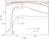 |
Fig. 2 Photospheric profiles for M = 10 M⊙ and a∗ = 0.0. |
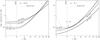 |
Fig. 3 Profiles of the disk angular momentum for α = 0.01 (left) and α = 0.1 (right panel) at different accretion rates in the Schwarzschild metric. The spin of the BH a∗ = 0. |
5. Results for bh spin evolution
Using the slim disk solutions described in the previous section, we solve Eqs. (7) and (8) using a regular Runge-Kutta method of the 4th order. To calculate the integrals (Eqs. (11) and (12)), we use the alternative extended Simpson’s rule (Press 2002) with 100 grid points in , , and radius r. We carried out tests to verify that this number is sufficient for convergence.
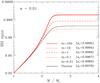 |
Fig. 4 Spin evolution for α = 0.01. |
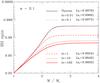 |
Fig. 5 Spin evolution for α = 0.1. |
In Figs. 4 and 5, we present the BH spin evolution for α = 0.01 and 0.1, respectively. The red lines show the results for different accretion rates, while the black line indicates the classical Thorne (1974) solution based on the Novikov & Thorne (1973) model of thin accretion disk. Our low accretion rate limit does not perfectly agree with the black line as the slim disk model does not account for the angular momentum carried away by radiation. As a result, the low-luminosity slim disk solutions slightly overestimate the emitted flux (by no more than a few percent) leading to stronger deceleration of the BH by radiation. The Thorne (1974) result is the proper limit for the lowest accretion rates. When the accretion rate is high enough (e.g., ṁ > 0.1), the impact of the omitted angular momentum flux is overwhelmed by the modification of the disk structure introduced by advection.
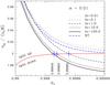 |
Fig. 6 The rate of spin-up or spin-down by “pure” accretion (radiation neglected) for α = 0.01. Profiles for five accretion rates are presented. Their intersections with the red line (marked with blue crosses) correspond to equilibrium states. For the two lowest accretion rates, the equilibrium state is never reached (a∗ → 1). |
BH spin terminal values.
To study the impact of radiation on BH spin evolution in detail, we calculated the rate of BH spin-up for the “pure” accretion of matter (without accounting for the impact of radiation). In that case, the BH spin evolution is given by (compare Eq. (7))  (45)In Figs. 6 and 7, we plot with black lines the first term on the right hand side of the above equation for different accretion rates and values of α. The red lines in these plots show the absolute value of the second term. The intersections of the black and red lines denote the equilibrium states, i.e., the limiting values of BH spin for pure accretion. These values differ significantly from the previously discussed results only at low accretion rates. In contrast, at high accretion rates radiation has little impact on the spin evolution and the value of terminal spin is mostly determined by the properties of the flow. In Fig. 8, we plot the radiation impact parameter ξ, defined as the ratio of the disk-driven terms on the right hand sides of Eqs. (7) and (45)
  (46)If the captured radiation significantly decelerates the BH spin-up, this ratio drops below unity. On the other hand, it is close to unity when the BH spin evolution is unaffected by the radiation. According to Fig. 8, the latter is the case for the highest accretion rates, independently of α.
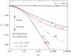 |
Fig. 8 Radiation impact factor ξ (Eq. (46)) for different accretion rates and values of α. The dotted line corresponds to the thin-disk induced spin evolution. For ξ ≈ 1, spin evolution is unaffected by radiation. Stars denote the equilibrium states (compare Table 1). |
In Table 1, we list the resulting values of the terminal BH spin for all the models considered. The first column gives the results for our fiducial model (A) including Thorne’s capture function and emission from the photosphere at the appropriate radial velocity.
The second column presents results obtained assuming the same (Thorne’s) capture function and profiles of emission, angular momentum, and radial velocity as in model A, but assuming the emission takes place from the equatorial plane instead of the photosphere. The resulting terminal spin values are equal, up to 4 decimal digits, to the values obtained with the fiducial model. This result is as expected for the lowest accretion rates, where the photosphere is located very close to the equatorial plane. For the highest accretion rates, the location of the emission has no impact on the BH spin-up, as the spin evolution is driven by the flow itself and the effects of radiation are negligible. However, for moderate accretion rates one could have expected significant change in the terminal spin. We find that the location of the photosphere has little impact on the resulting BH spin regardless of the accretion rate.
Our third model (V) neglects the flow radial velocity when the radiative terms are evaluated. Similar arguments to those given in the previous paragraph apply. For the lowest accretion rates, the radial velocity is negligible and therefore should have no impact on the resulting spin. For the highest accretion rates, the spin-up process depends only on the properties of the flow. Once again, however, the impact of this assumption on moderate accretion rates is not obvious. The radial velocity turns out to be of little importance for the calculation of the terminal spin (only for α = 0.1 and moderate accretion rates the difference between models A and V is higher than 0.01%).
In the fourth and fifth columns of Table 1, results for models with the same assumptions as the fiducial model, but with different capture functions are presented. The first alternative capture function (C1) assumes that the angular momentum and energy of all photons returning to the disk are added to that of the BH. This assumption has a strong impact on the spin evolution – the terminal spin values are higher, sometimes approaching a∗ = 1. This may seem surprising because in the classical approach the captured photons are responsible for decelerating the spin-up. This deceleration occurs because the cross-section (with respect to the BH) of photons moving “against” the frame dragging is larger than of photons following the BH sense of rotation. As frame dragging is involved, this effect is significant only in the vicinity of the BH horizon. For our model C1, however, the probability of photons returning to the disk does not differ appreciably for co- and counter-rotating photons, as they both hit the disk surface mostly at large radii.
The other capture function (C2) assumes, in contrast, that all returning photons are re-emitted from the disk with their original angular momentum and energy (and never fall onto the BH). This assumption cuts off the photons that would hit the BH in the fiducial model after crossing the disk surface, thus leading to a smaller radiative deceleration and higher values of the terminal spin parameter. However, these changes are insignificant, because most of the original photons hit the BH directly, along slightly curved trajectories. Only for α = 0.1 and moderate accretion rates do the terminal spin values differ in the 4th decimal digit.
Neither of the models with a modified capture functions is self-consistent. To account properly for the returning radiation, one has to modify the disk equations by introducing appropriate terms for the outgoing and incoming fluxes of angular momentum and additional radiative heating. No such model for advective, optically thick accretion disk has been constructed. The emission profile should be significantly affected (especially inside the marginally stable orbit) by the returning radiation, leading to different rates of deceleration by photons. In view of our results for models C1 and C2, as well as the results of Li et al. (2005), one may expect the final spin values for super-critical accretion flows to be slightly higher than the ones obtained in this work.
The last column of Table 1 gives terminal spin values for “pure” accretion (radiation neglected). Under these assumptions, the BH spin could reach a∗ = 1 for sub-Eddington accretion rates as there are no photons that could decelerate and stop the spin-up process. As discussed above, for the highest accretion rates the resulting BH spin values agree with the values obtained for the fiducial model as radiation has little impact on spin evolution in this regime.
6. Discussion
We have studied the spin evolution of black holes undergoing disk accretion assuming that the angular momentum and energy carried by both the flow and the emitted photons are the only factors affecting the BH rotation. We have generalized the original study of Thorne (1974) to high accretion rates by applying a relativistic, advective, optically thick slim accretion disk model. Assuming isotropic photon emission from the disk (no limb darkening), we have shown that:
-
(i)
the terminal value of BH spin depends on the accretion rate forṁ ≳ 1;
-
(ii)
the terminal spin value is very sensitive to the assumed value of the viscosity parameter α – for α ≲ 0.01 the BH is spun up to a∗ > 0.9978 for high accretion rates, while for α ≳ 0.1 to a∗ < 0.9978;
-
(iii)
with a low value of α and high accretion rates, the BH may be spun up to spins significantly higher than the canonical value a∗ = 0.9978 (e.g., to a∗ = 0.9994 for α = 0.01 and ṁ = 10) but, under reasonable assumptions, BH cannot be spun up arbitrarily close to a∗ = 1;
-
(iv)
BH spin evolution is hardly affected by the emitted radiation for high (ṁ ≳ 10) accretion rates (the terminal spin value is determined by the flow properties only);
-
(v)
for all accretion rates, neither the photosphere profile nor the profile of radial velocity significantly affects the spin evolution.
We point out that the inner edge of an accretion disk cannot be uniquely defined for super-critical accretion (Abramowicz et al. 2010), as opposed to geometrically thin disks where the inner edge is uniquely located at the marginally stable orbit (Rms). In the thin-disk case, the BH spin evolution is determined by the flow properties at this particular radius (as there is no torque between the marginally stable orbit and BH horizon) and the profile of emission (terminating at Rms). For super-critical accretion rates, however, one cannot distinguish a particular inner edge that is relevant to studying BH spin evolution. On the one hand, the values of the specific energy (ut) and the angular momentum (uφ) remain constant within the stress inner edge. On the other, the radiation is emitted outside the radiation inner edge. These inner edges do not coincide as they are related to different physical processes (Abramowicz et al. 2010).
Our study was based on a semi-analytical, hydrodynamical model of an accretion disk that makes a number of simplifying assumptions such as stationarity, no returning radiation, α-viscosity prescription, no wind outflows, and neglects interactions of large-scale magnetic fields interactions with BHs. One has to be aware that the precise values of the terminal spin parameter are very sensitive to the flow and emission properties, as well as to the impact of magnetic fields (e.g., by means of the Blandford-Znajek process). The slim disk model only approximates the real accretion flows driven by magnetically-induced turbulence – in this respect it is no different from MHD simulations. Its applicability is limited by the adopted assumptions. The lack of magnetic fields may result in improper description of the innermost part of the flow where the disk may be be magnetically supported (Narayan et al. 2003; Igumenshchev et al. 2003; Meier 2005; Fragile & Meier 2009). The model also does not account for the returning radiation that may affect the accretion flow. However, super-critical accretion is expected to be radiatively inefficient and therefore the impact of radiation should not be large. Despite these limitations, our study shows that Thorne’s canonical value for BH spin (a∗ = 0.9978) may be exceeded under certain conditions.
Of more fundamental interest is that the proper geodesic distances D between the marginally stable orbit (the innermost stable orbit, ISCO) and several other special Keplerian orbits relevant to accretion disk structure tend to infinity D → ∞ when a∗ → 1 (Bardeen et al. 1972).
Acknowledgments
This work was supported in part by Polish Ministry of Science grants N203 0093/1466, N203 304035, N203 380336, and N N203 381436. J.P.L. acknowledges support from the French Space Agency CNES, MB from GAČR 205/07/0052.
References
- Abramowicz, M. A., & Lasota, J. P. 1980, Acta Astron., 30, 35 [NASA ADS] [Google Scholar]
- Abramowicz, M. A., Chen, X.-M., Granath, M., & Lasota, J.-P. 1996, ApJ, 471, 762 [NASA ADS] [CrossRef] [Google Scholar]
- Abramowicz, M. A., Jaroszyński, M., Kato, S., et al. 2010, A&A, 521, A15 [NASA ADS] [CrossRef] [EDP Sciences] [Google Scholar]
- Bañados, M., Silk, J., & West, S. M. 2009, Phys. Rev. Lett., 103, 111102 [NASA ADS] [CrossRef] [MathSciNet] [PubMed] [Google Scholar]
- Bardeen, J. M. 1970, Nature, 226, 64 [NASA ADS] [CrossRef] [PubMed] [Google Scholar]
- Bardeen, J. M., Press, W. H., & Teukolsky, S. A. 1972, ApJ, 178, 347 [NASA ADS] [CrossRef] [Google Scholar]
- Bardeen, J. M., Carter, B., & Hawking, S. W. 1973, Comm. Math. Phys., 31, 161 [Google Scholar]
- Belczynski, K., Taam, R. E., Rantsiou, E., & van der Sluys, M. 2008, ApJ, 682, 474 [NASA ADS] [CrossRef] [Google Scholar]
- Berti, E., & Volonteri, M. 2008, ApJ, 684, 822 [NASA ADS] [CrossRef] [Google Scholar]
- Bursa, M. 2006, Ph.D. Thesis [Google Scholar]
- Carter B. 1973, in Black Holes (Les Astres Occlus), ed. C. DeWitt, & B. S. DeWitt (Gordon and Breach Science Publishers), 57 [Google Scholar]
- Fanidakis, N., Baugh, C. M., Benson, A. J., et al. 2011, MNRAS, 410, 53 [NASA ADS] [CrossRef] [Google Scholar]
- Fragile, P. C., & Meier, D. L. 2009, ApJ, 693, 771 [NASA ADS] [CrossRef] [Google Scholar]
- Gammie, C. F., & Popham, R. 1998, ApJ, 498, 313 [NASA ADS] [CrossRef] [Google Scholar]
- Gammie, C. F., Shapiro, S. L., & McKinney, J. C. 2004, ApJ, 602, 312 [NASA ADS] [CrossRef] [Google Scholar]
- Ghosh, P., & Abramowicz, M. A. 1997, MNRAS, 292, 887 [NASA ADS] [CrossRef] [Google Scholar]
- Igumenshchev, I. V., Narayan, R., & Abramowicz, M. A. 2003, ApJ, 592, 1042 [NASA ADS] [CrossRef] [Google Scholar]
- Kato, S., Fukue, J., & Mineshige, S. 2008, Black-Hole Accretion Disks – Towards a New Paradigm, ed. S. F. J. M. S. Kato [Google Scholar]
- King, A. R., Pringle, J. E., & Hofmann, J. A. 2008, MNRAS, 385, 1621 [NASA ADS] [CrossRef] [Google Scholar]
- Kozłowski, M., Jaroszyński, M., & Abramowicz, M. A. 1978, A&A, 63, 209 [NASA ADS] [Google Scholar]
- Lasota, J. P. 1994, in Theory of Accretion Disks – 2, ed. W. J. Duschl, J. Frank, F. Meyer, E. Meyer-Hofmeister, & W. M. Tscharnuter, NATO ASIC Proc., 417: 341 [Google Scholar]
- Li, L.-X., Zimmerman, E. R., Narayan, R., & McClintock, J. E. 2005, ApJS, 157, 335 [NASA ADS] [CrossRef] [Google Scholar]
- Livio, M., Ogilvie, G. I., & Pringle, J. E. 1999, ApJ, 512, 100 [NASA ADS] [CrossRef] [Google Scholar]
- McKinney, J. C., & Narayan, R. 2007, MNRAS, 375, 513 [NASA ADS] [CrossRef] [Google Scholar]
- Meier, D. L. 2005, Ap&SS, 300, 55 [NASA ADS] [CrossRef] [Google Scholar]
- Misner, C. W., Thorne, K. S., & Wheeler, J. A. 1973 (San Francisco: W.H. Freeman and Co.) [Google Scholar]
- Moderski, R., Sikora, M., & Lasota, J.-P. 1998, MNRAS, 301, 142 [NASA ADS] [CrossRef] [Google Scholar]
- Narayan, R., Igumenshchev, I. V., & Abramowicz, M. A. 2003, PASJ, 55, L69 [NASA ADS] [Google Scholar]
- Novikov, I. D., & Thorne, K. S. 1973, in Black Holes (Les Astres Occlus), ed. C. DeWitt, & B. S. DeWitt (Gordon and Breach Science Publishers), 343 [Google Scholar]
- Ohsuga, K. 2007, ApJ, 659, 205 [NASA ADS] [CrossRef] [Google Scholar]
- Popham, R., & Gammie, C. F. 1998, ApJ, 504, 419 [NASA ADS] [CrossRef] [Google Scholar]
- Press, W. H. 2002, Numerical recipes in C++: the art of scientific computing by William H. Press [Google Scholar]
- Shakura, N. I., & Sunyaev, R. A. 1973, A&A, 24, 337 [NASA ADS] [Google Scholar]
- Sądowski, A. 2009, ApJS, 183, 171 [NASA ADS] [CrossRef] [Google Scholar]
- Sądowski, A., Abramowicz, M., Bursa, M., et al. 2011, A&A, 527, A17 [NASA ADS] [CrossRef] [EDP Sciences] [Google Scholar]
- Thorne, K. S. 1974, ApJ, 191, 507 [Google Scholar]
- Volonteri, M., Madau, P., Quataert, E., & Rees, M. J. 2005, ApJ, 620, 69 [NASA ADS] [CrossRef] [Google Scholar]
- Volonteri, M., Sikora, M., & Lasota, J.-P. 2007, ApJ, 667, 704 [NASA ADS] [CrossRef] [Google Scholar]
- Wald, R. W. 1984 (University of Chicago Press) [Google Scholar]
Appendix A: The tetrad for an observer instantaneously located at the photosphere
Our aim is to derive the tetrad of an observer moving along the photosphere that would depend only on the quantities that are typically calculated in accretion disk models, i.e., on the radial and azimuthal velocities of gas and the location of the disk photosphere.
The metric considered here is the Kerr geometry gik in the Boyer-Lindquist coordinates [t,φ,r,θ]. The signature adopted is + − − − . As in Carter’s Les Houches lectures (Carter 1972), we consider two fundamental planes; the symmetry plane ![Mathematical equation: \appendix \setcounter{section}{1} \hbox{${\cal S}_0 = [t, \phi]$}](/articles/aa/full_html/2011/08/aa16702-11/aa16702-11-eq164.png) and the meridional plane ℳ∗ = [r,θ]. (Four)-vectors that belong to the plane
and the meridional plane ℳ∗ = [r,θ]. (Four)-vectors that belong to the plane  , are denoted by the subscript 0, and vectors that belong to the plane ℳ∗, will be denoted by the subscript ∗ . For example, the two Killings vectors are
  ,
,  . We note that for any pair
  one has,
A.1. Stationary and axially symmetric photosphere
A.1.1. The photosphere
Numerical solutions of slim accretion disks provide the location of the photosphere given by HPh(r) = rcosθ. This may be substituted into rcosθ − HPh(r) ≡ F(r,θ) = 0. The normal vector to the photosphere surface has the [r,θ] components ![Mathematical equation: \appendix \setcounter{section}{1} \begin{equation} N_*^i = \tilde N_* \left[\pder F r,\pder F\theta\right]=\tilde N_*' \left[\der{\theta_*}{r},1\right], \end{equation}](/articles/aa/full_html/2011/08/aa16702-11/aa16702-11-eq177.png) (A.1)where
(A.1)where  (A.2)is the derivative of the angle defining the location of the photosphere at a given radial coordinate [cosθ∗(r) = HPh(r)/r]. Its non-zero components after normalization [(N∗N∗) = − 1] are
 ![Mathematical equation: \appendix \setcounter{section}{1} \begin{eqnarray} N_*^r &=& \der{\theta_*} r\left(-g_{\theta\theta}\right)^{-1/2} \left[1+\frac{g_{rr}}{g_{\theta\theta}} \left(\der{\theta_*}r\right)^2\right]^{-1/2}, \nonumber\\[1.5mm] N_*^\theta &=& \left(-g_{\theta\theta}\right)^{-1/2} \left[1+\frac{g_{rr}}{g_{\theta\theta}}\left(\der{\theta_*}r\right)^2\right]^{-1/2}\cdot \end{eqnarray}](/articles/aa/full_html/2011/08/aa16702-11/aa16702-11-eq181.png) (A.3)There are two unique vectors S∗ confined to the [r,θ] plane that are orthogonal to N∗ (and therefore are tangential to the surface). From (S∗N∗) = 0 and (S∗S∗) = − 1, one obtains the non-zero components of one of them.
(A.3)There are two unique vectors S∗ confined to the [r,θ] plane that are orthogonal to N∗ (and therefore are tangential to the surface). From (S∗N∗) = 0 and (S∗S∗) = − 1, one obtains the non-zero components of one of them. ![Mathematical equation: \appendix \setcounter{section}{1} \begin{eqnarray} \label{e.Sstar} S_*^r &=& \left(g_{rr}\right)^{-1} \left[-\frac1{g_{rr}}-\frac1{g_{\theta\theta}}\left(\der{\theta_*}r\right)^2\right]^{-1/2}, \nonumber\\[1.5mm] S_*^\theta &=& -\left(g_{\theta\theta}\right)^{-1} \left(\der{\theta_*}r\right)\left[-\frac1{g_{rr}}-\frac1{g_{\theta\theta}}\left(\der{\theta_*}r\right)^2\right]^{-1/2}. \end{eqnarray}](/articles/aa/full_html/2011/08/aa16702-11/aa16702-11-eq186.png) (A.4)
(A.4)
A.1.2. The four-velocity of matter and the tetrad
The four-velocity u of gas moving along the photosphere may be decomposed into  (A.5)where
  (A.6)is the four-velocity of an observer with azimuthal motion only. The normalization constant
  comes from (u0u0) = 1 and equals
 ![Mathematical equation: \appendix \setcounter{section}{1} \begin{equation} \tilde A_0 = \left[g_{tt}+\Omega g_{\phi\phi}(\Omega-2\omega)\right]^{-1/2}. \end{equation}](/articles/aa/full_html/2011/08/aa16702-11/aa16702-11-eq192.png) (A.7)It is useful to construct a spacelike vector (κ0) confined to the [t,φ] plane, that is perpendicular to both u and u0. From (κκ) = − 1 and, e.g., (κu0) = 0, we have
(A.7)It is useful to construct a spacelike vector (κ0) confined to the [t,φ] plane, that is perpendicular to both u and u0. From (κκ) = − 1 and, e.g., (κu0) = 0, we have ![Mathematical equation: \appendix \setcounter{section}{1} \begin{equation} \kappa_0^i = \frac{\left(l\eta^i+\xi^i\right)}{\left[-g_{\phi\phi}(1-\Omega l)(1-\omega l)\right]^{1/2}}, \end{equation}](/articles/aa/full_html/2011/08/aa16702-11/aa16702-11-eq198.png) (A.8)where l = uφ/ut is the specific angular momentum. We note that the set of vectors
(A.8)where l = uφ/ut is the specific angular momentum. We note that the set of vectors ![Mathematical equation: \appendix \setcounter{section}{1} \hbox{$[u_0^i, N_*^i, \kappa_0^i, S_*^i]$}](/articles/aa/full_html/2011/08/aa16702-11/aa16702-11-eq200.png) already forms the desired tetrad that is valid for the pure rotation (ur = 0) case.
already forms the desired tetrad that is valid for the pure rotation (ur = 0) case.
The normalization condition (uu) = 1 gives ![Mathematical equation: \appendix \setcounter{section}{1} \begin{equation} \tilde A = \left[g_{tt} + \Omega g_{\phi\phi}(\Omega-2\omega)-v^2\right]^{-1/2}, \end{equation}](/articles/aa/full_html/2011/08/aa16702-11/aa16702-11-eq203.png) (A.9)where v is related to the radial component of the gas four-velocity ur by
(A.9)where v is related to the radial component of the gas four-velocity ur by ![Mathematical equation: \appendix \setcounter{section}{1} \begin{equation} v^2 = \frac{\left(u^r/S^r_*\right)^2\left[g_{tt}+\Omega g_{\phi\phi} (\Omega - 2\omega)\right]}{1+\left(u^r/S^r_*\right)^2}\cdot \label{e.V} \end{equation}](/articles/aa/full_html/2011/08/aa16702-11/aa16702-11-eq206.png) (A.10)The vectors we have just calculated (u,κ0) are both orthogonal to N∗ since (N∗S∗) = 0. To complete the tetrad, we need one more spacelike vector (S) that is orthogonal to these three. We decompose this into
(A.10)The vectors we have just calculated (u,κ0) are both orthogonal to N∗ since (N∗S∗) = 0. To complete the tetrad, we need one more spacelike vector (S) that is orthogonal to these three. We decompose this into  (A.11)The orthogonality conditions (κ0S) = 0 and (N∗S) = 0 immediately implies that γ = β = 0. The only non-trivial condition is that (uS) = 0. Together with (SS) = − 1, it implies that
  (A.12)The vectors ui,
  ,
,  , and Si form an orthonormal tetrad in the Kerr spacetime
 ![Mathematical equation: \appendix \setcounter{section}{1} \begin{equation} \label{velocity-tetrad} e^i_{(A)} = \left[u^i, N_*^i, \kappa_0^i, S^i\right]. \end{equation}](/articles/aa/full_html/2011/08/aa16702-11/aa16702-11-eq221.png) (A.13)This tetrad is known directly from the slim disk solutions, as it depends on the calculated quantities (ur, Ω, l and θ∗(r)) only. Any spacetime vector Xi could be uniquely decomposed into this tetrad with
(A.13)This tetrad is known directly from the slim disk solutions, as it depends on the calculated quantities (ur, Ω, l and θ∗(r)) only. Any spacetime vector Xi could be uniquely decomposed into this tetrad with  .
.
A.2. The general case
We here assume nothing about the four-velocity of matter ui and the location of photosphere. Both may be non-stationary and non-axially symmetric. Following the same framework as in Sect. A.1, we describe how to obtain the tetrad of an observer instantaneously located at the photosphere that depends only on the quantities calculated by accretion disk models.
A.2.1. The four velocity
As in Sect. A.1.2, we may always uniquely decompose ui, a general timelike unit vector, into  (A.14)where
  is a timelike unit vector, and
  is a spacelike unit vector. Equation (A.14) uniquely defines the two vectors , and the two scalars
  , v. The vectors and scalars
  (A.15)can be calculated from known quantities given by slim disk model solutions.
The four-velocity (A.14) also defines the instantaneous 3-space of the comoving observer with the metric γik and the projection tensor 
![Mathematical equation: \appendix \setcounter{section}{1} \begin{eqnarray} \gamma_{ik} &=& g_{ik} - u_i\,u_k,\\[1.5mm] \label{comoving-metric} h^i_{k} &=& \delta^i_{k} - u^i\,u_k. \end{eqnarray}](/articles/aa/full_html/2011/08/aa16702-11/aa16702-11-eq234.png) We define the two unit vectors and by the unique condition
We define the two unit vectors and by the unique condition  (A.18)As before, the four vectors
 ![Mathematical equation: \appendix \setcounter{section}{1} \begin{equation} \label{velocity-tetrad2} e^i_{(A)} = \left[u_0^i, N_*^i, \kappa_0^i, S_*^i\right], \end{equation}](/articles/aa/full_html/2011/08/aa16702-11/aa16702-11-eq236.png) (A.19)form an orthonormal tetrad of an observer with the four-velocity can calculated from the solutions of the slim-disk equations.
(A.19)form an orthonormal tetrad of an observer with the four-velocity can calculated from the solutions of the slim-disk equations.
A.2.2. The photosphere
In the most general case of a non-stationary and non-axially symmetric photosphere, the location of the photosphere may be described by the condition  (A.20)The vector
  normal to the photosphere has the components
 ![Mathematical equation: \appendix \setcounter{section}{1} \begin{equation} \label{normal-photosphere} {\tilde N}^i = \left[\frac{\partial F}{\partial t}, \frac{\partial F}{\partial \phi}, \frac{\partial F}{\partial r}, \frac{\partial F}{\partial \theta} \right] \end{equation}](/articles/aa/full_html/2011/08/aa16702-11/aa16702-11-eq239.png) (A.21)which may be calculated from slim disk solutions.
(A.21)which may be calculated from slim disk solutions.
We project  into the instantaneous 3-space of the comoving observer (A.17) and normalize to a unit vector after the projection to obtain
  (A.22)In terms of the tetrad in Eq. (A.19), a vector Ni constructed in this way has the decomposition
 ![Mathematical equation: \appendix \setcounter{section}{1} \begin{equation} \label{projected-normal-decomposition} N^i = {\tilde N}\,\left[\alpha\, \left(u_0^i\right) + 1\, \left(N_*^i\right) + \gamma\, \left(\kappa_0^i\right) + \delta\, \left(S_*^i\right)\right]. \end{equation}](/articles/aa/full_html/2011/08/aa16702-11/aa16702-11-eq243.png) (A.23)The components
(A.23)The components  are known.
A.2.3. The tetrad
We now decompose the four vectors, the first two of which we have derived, the next two guessed (but the guess should be obvious): ![Mathematical equation: \appendix \setcounter{section}{1} \begin{eqnarray} \label{final-tetrad-u} u^i &=& {\tilde A}\left[1 \left(u_0^i\right) + 0 \left(N_*^i\right) + 0 \left(\kappa_0^i\right) + V \left(S_*^i\right)\right], \\[1.5mm] \label{final-tetrad-N} N^i &=& {\tilde N}\left[\alpha \left(u_0^i\right) + 1 \left(N_*^i\right) + \gamma \left(\kappa_0^i\right) + \delta \left(S_*^i\right)\right], \\[1.5mm] \label{final-tetrad-K} \kappa^i &=& {\tilde \kappa} \left[0 \left(u_0^i\right) + b \left(N_*^i\right) + 1 \left(\kappa_0^i\right) + 0 \left(S_*^i\right)\right], \\[1.5mm] \label{final-tetrad-S} S^i &=& {\tilde S} \left[A \left(u_0^i\right) + B \left(N_*^i\right) + C \left(\kappa_0^i\right) + 1 \left(S_*^i\right)\right]. \end{eqnarray}](/articles/aa/full_html/2011/08/aa16702-11/aa16702-11-eq245.png) The four unknown components, b, A, B, C one calculates from the following four non-trivial orthogonality conditions ((uκ) ≡ 0 by construction, cf. (A.24) and (A.26))
The four unknown components, b, A, B, C one calculates from the following four non-trivial orthogonality conditions ((uκ) ≡ 0 by construction, cf. (A.24) and (A.26))  (A.28)and the two unknown factors
  and
and  from the following two normalization conditions
  (A.29)The conditions (A.28) and (A.29) are given by linear equations.
Equations (A.24)–(A.29) define the tetrad  of an observer comoving with matter, and instantaneously located at the photosphere:
 ![Mathematical equation: \appendix \setcounter{section}{1} \begin{equation} \label{tetrad-final-final} e_{(A)}^{i} = \left[u^i, N^i, \kappa^i, S^i\right]. \end{equation}](/articles/aa/full_html/2011/08/aa16702-11/aa16702-11-eq256.png) (A.30)Both the matter and the photosphere move in a general manner. The zenithal direction in the local observer’s sky is given by Ni.
(A.30)Both the matter and the photosphere move in a general manner. The zenithal direction in the local observer’s sky is given by Ni.
Appendix B: Integration over the world-tube of the photosphere
For stationary and axially symmetric models, we define:
-
 unit vector orthogonal to the photosphere, which is in the [r,θ] plane;
 -
 unit vector orthogonal to Ni, which is in the [r,θ] plane;
 -
ui = four-velocity of matter, which is in the [t,φ,r,θ] space-time;
-
 unit vector orthogonal to Ui, which is in the [t,φ] plane;
 -
Si = unit vector orthogonal to Ui, Ni and κi, which is in the [t,φ,r,θ] space-time;
-
![Mathematical equation: \appendix \setcounter{section}{2} \hbox{$e_{(A)}^{i} = [u^i, N^i,\kappa^i, S^i] =$}](/articles/aa/full_html/2011/08/aa16702-11/aa16702-11-eq268.png) the tetrad comoving with an observer located in the photosphere.
the tetrad comoving with an observer located in the photosphere.
The integration of a vector (...)i over the 3D hypersurface ℋ orthogonal to Ni (i.e. the 3D world-tube of the photosphere) may be symbolically written as  (B.1)where dS is the “volume element” in ℋ.
Obviously, the hypersurface ℋ is spanned by the three vectors [ui,κi,Si]N. Each of them is a linear combination of ![Mathematical equation: \appendix \setcounter{section}{2} \hbox{$[\eta^i, \xi^i, S_*^i]_{N}$}](/articles/aa/full_html/2011/08/aa16702-11/aa16702-11-eq274.png) , and each of the three vectors from is orthogonal to Ni.
, and each of the three vectors from is orthogonal to Ni.
Therefore, one may say that the hypersurface ℋ is spanned by . It is convenient to write  (B.2)where dR is the line element along the vector
  , i.e. along the photosphere in the [r,θ] plane, with θ = θ∗(r) defining the location of the photosphere, and dA being the surface element on the [t,φ] plane.
To calculate dA we imagine an infinitesimal parallelogram with sides that are located along the t = const. and φ = const. lines. The proper lengths of the sides are du = | gtt | 1/2dt and dv = | gφφ | 1/2dφ, respectively, and therefore dA, which is just the area of the parallelogram, is given by  (B.3)where α is the angle between the two sides. Obviously, the cosine of this angle is given by the scalar product of the two unit vectors ni and xi pointing in the [t,φ] plane into the t and φ directions respectively. These vectors are given by (note that ni = ZAMO)
  (B.4)Because
  and
and  , one may write
  (B.5)Therefore,
  (B.6)and
  (B.7)Inserting this into the formula for dA, we get
  . The final formula for dS is,
  (B.8)
(B.8)
All Tables
All Figures
|
Fig. 1 Flux profiles for M = 10 M⊙ and a∗ = 0.0. |
| In the text | |
|
Fig. 2 Photospheric profiles for M = 10 M⊙ and a∗ = 0.0. |
| In the text | |
|
Fig. 3 Profiles of the disk angular momentum for α = 0.01 (left) and α = 0.1 (right panel) at different accretion rates in the Schwarzschild metric. The spin of the BH a∗ = 0. |
| In the text | |
|
Fig. 4 Spin evolution for α = 0.01. |
| In the text | |
|
Fig. 5 Spin evolution for α = 0.1. |
| In the text | |
|
Fig. 6 The rate of spin-up or spin-down by “pure” accretion (radiation neglected) for α = 0.01. Profiles for five accretion rates are presented. Their intersections with the red line (marked with blue crosses) correspond to equilibrium states. For the two lowest accretion rates, the equilibrium state is never reached (a∗ → 1). |
| In the text | |
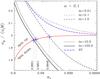 |
Fig. 7 Same as Fig. 6 but for α = 0.1. |
| In the text | |
|
Fig. 8 Radiation impact factor ξ (Eq. (46)) for different accretion rates and values of α. The dotted line corresponds to the thin-disk induced spin evolution. For ξ ≈ 1, spin evolution is unaffected by radiation. Stars denote the equilibrium states (compare Table 1). |
| In the text | |
Current usage metrics show cumulative count of Article Views (full-text article views including HTML views, PDF and ePub downloads, according to the available data) and Abstracts Views on Vision4Press platform.
Data correspond to usage on the plateform after 2015. The current usage metrics is available 48-96 hours after online publication and is updated daily on week days.
Initial download of the metrics may take a while.