| Issue |
A&A
Volume 531, July 2011
|
|
|---|---|---|
| Article Number | A83 | |
| Number of page(s) | 6 | |
| Section | Stellar atmospheres | |
| DOI | https://doi.org/10.1051/0004-6361/201116911 | |
| Published online | 16 June 2011 | |
The Hα Balmer line as an effective temperature criterion
I. Calibration using 1D model stellar atmospheres
1
Observatoire de Paris, GEPI, CNRS UMR 8111, Université Denis Diderot, 61 Av. de l’Observatoire, 75014 Paris, France
e-mail: roger.cayrel@obspm.fr
2
Observatoire de Paris, GEPI, CNRS UMR 8111, Université Denis Diderot, 5 place J. Janssen, 92195 Meudon Principal Cedex, France
3
Institut d’Astrophysique de Paris, UMR 7095, CNRS, Université Pierre et Marie Curie, 98bis boulevard Arago, 75014 Paris, France
4
Observatoire de Paris, LERMA, UMR 8112, Université Pierre et Marie Curie, CNRS, 5 place J. Janssen, 92195 Meudon Principal Cedex, France
Received: 17 March 2011
Accepted: 14 April 2011
Aims. We attempt to derive the true effective temperature of a star from the spectroscopic observation of its Hα Balmer line profile.
Methods. The method is possible thanks to advances in two respects. First there have been progresses in the theoretical treatment of the broadening mechanisms of Hα. Second, there has been a rapid increase in the number of stars with an apparent diameter measured with an accuracy of the order of 1 percent, enabling us to obtain an accurate effective temperature Teff for a dozen of stars using the direct method by means of combining the apparent diameter and the bolometric flux.
Results. For the eleven stars with an accurate effective temperature derived from their apparent angular diameter we determined the effective temperature of the Kurucz Atlas9 model that provides the best fit of the computed theoretical Hα profile (using the recent theoretical advances) with the corresponding observed profile, extracted from the S4N spectroscopic database. The two sets of effective temperatures have a significant offset, but are tightly correlated, with a correlation coefficient of 0.9976. The regression straight line of Teff(direct) versus Teff(Hα) enables us to reach the true effective temperature from the spectroscopic observation of the Hα profile, with an rms error of only 30 K. This provides a way of obtaining the true effective temperature of a reddened star.
Conclusions. We succeeded in obtaining empirically the true stellar effective temperature from Hα profile using Kurucz’s Atlas9 grid of 1D model atmospheres. Full understanding of the difference between Teff(direct) and Teff(Hα) would require a 3D approach, with radiative hydrodynamical models, which will be the subject of a future paper.
Key words: stars: atmospheres / stars: fundamental parameters / line: profiles
© ESO, 2011
1. Introduction
Many authors use the Hα Balmer line as an effective temperature criterion (Fuhrmann et al. 1993; 1997; Gehren et al. 2006; Gratton et al. 2001; Bonifacio et al. 2007). The advantage of Hα is its full independence of interstellar reddening, a significant advantage over photometric indices. However, two events justify a reconsideration of the determination of effective temperatures from Hα.
The first event has been recent progress in the physics of line formation. Barklem et al. (2000; 2002) achieved an important revision of the cross-section of the self-resonance broadening of Hα by collisions with neutral hydrogen atoms in the ground state, and significantly improved the accuracy of previous adopted values such as the one of Ali-Griem (1966). Allard et al. (2008) then improved the values of Barklem et al., taking into account the weaker transitions 3p-2s and 3s-2p, not included in Barklem et al. (2000), and using Spielfiedel et al. (2004) ab initio interaction potentials. This again increased the width of the Hα collisional profile exacerbating the difference between the observed profile of Hα in the Sun and the one computed with current 1D models, wich was not the expected result of an improved theoretical treatment. Using the so-called model microfield method (here MMM), from Brissaud & Frisch (1971), Stehlé & Hutcheon (1999) have put the calculation of the Stark broadening on a firmer foot.
The changes introduced by this approach (MMM), compared to VCS tables (Vidal, Cooper & Smith 1973), mainly concern the line center. Thus, their impact on the part of the Hα line profile that we use (3 to 15 Å from the line center) is less than the changes brought by the collisional broadening described above caused by neutral hydrogen atoms. However, MMM still improves the accuracy of the theoretical profile, placing a tighter constraint on the effective temperature. The details of the fitting process of the observed profile with the theoretical one, computed with the two recent improvements, are given in Sect. 2.
The second event has been the enormous gain in the accuracy of angular diameter measurements of stars by interferometric methods. This has made it possible to directly measure the stellar effective temperatures with the relation  (1)where fbol is the apparent bolometric flux of the object, θ its limb-darkened angular diameter, and σ the Stefan-Boltzmann constant, all in CGS units. This allows us to calibrate any effective temperature criterion with directly measured effective temperatures in the range 5000−7000 K, instead of using the infrared flux method, for which several discrepant scales are in use. Section 3 describes the implementation of the direct method. Section 4 calibrates the Hα effective temperatures with the help of the ones obtained with the direct method. Section 5 presents some considerations of the halo metal-poor stars that are absent from our calibration. Section 6 discusses the cause of the offset between the two temperatures. Section 7 presents the conclusions of our paper.
2. Effective temperatures from the Hα fitting procedure
2.1. Observations
The observation of Hα profiles is not straightforward. The main difficulty comes from most high-resolution observations being now done with cross-dispersed spectrographs, with a continuum modulated by the efficiency of the blaze of the orders, varying by 50 percent from one end to the other of each order. This modulation is theoretically corrected by flat-fields, although the path of the light generally differs between the two beams and order merging is always a problem. We decided, after several attempts, to use the homogeneous sample of the S4N library (Allende Prieto et al. 2004), which has an exceptional quality in this respect, and the signal-to-noise ratio required. The spectra have been taken at the McDonald Observatory of the University of Texas for the northern stars, and at ESO (FEROS spectrograph) for the southern stars. However, owing to instrumental difficulties1, we removed the southern stars from our program.
The Sun and the ten stars of the S4N catalogue with a measured angular diameter of accuracy higher than 2 percent, constitute our calibration sample for converting the Hα profile into true effective temperatures. They are listed in Table 2.
2.2. Model atmosphere
Our choice was to use Kurucz ATLAS9, BALMER9 codes2, mainly because they are the only ones that enable us to vary the sources, and introduce, for example, new broadening mechanisms for Hα or new convection treatments. We used the options of the mixing length theory (MLT) (Böhm-Vitense 1958), with l/Hp = 0.5, without overshooting, and y = 0.5. The parameter y is documented in Henyey et al. (1965) and characterizes the geometry and the transfer of radiation in convective bubbles. The choice of the MLT options is discussed in Heiter et al. (2002).
We modified BALMER9 incorporating the Stark broadening treatment of Stehlé & Hutcheon (1999), and the impact broadening of Allard et al. (2008) by neutral hydrogen collisions, which is found to be valid up to 20 Å from line center (cf. Fig. 11 in Allard et al.). The broadening mechanisms were quoted in the preceding section, and are now the most up to date.
2.3. The details of the fitting procedure and results
In the Hα profile, we select “windows” (as done in Barklem et al. 2002), where the Balmer line is not contaminated by other stellar lines. These windows are primarily selected in the Kurucz-Furenlid (2005) spectrum. The theoretical Hα profile computed with BALMER9, which treats only the hydrogen lines, can then be compared with the observed spectra within each window. We work with eight windows, four in the blue wing and four in the red wing visible in Figs. 1 and 2.
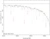 |
Fig. 1 Windows, delimitated by green vertical lines, and telluric lines, indicated by red arrows, on the blue wing of the observed solar Hα profile. |
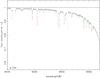 |
Fig. 3 Same as Fig. 1, but for the observed blue wing of Hα on the μ Cas spectrum. Clearly the bluest window (6549.50 Å) is entirely lost, because obliterated by a telluric line. |
In the solar spectrum, these windows are also free of telluric lines, which is obviously generally not true for stellar spectra, for which the radial velocity of the object with respect to Earth shifts the stellar lines with respect to the telluric lines. This obliges us to re-identify the telluric lines in the stellar spectra, and to check each window to verify whether it is still usable, or entirely lost by the contamination of the displaced telluric lines, as shown in Fig. 3.
For each star with a secure effective temperature from the direct method, we then extract from the literature, using the PASTEL data base (Soubiran et al. 2010), the physical atmospheric parameters of the star. We then compute the Hα profile for several effective temperatures of the model, keeping the other parameters log g, [M/H], and [ α/Fe ] at the values found in the most accurate recent determinations, given in PASTEL. The metallicity [M/H] is defined in the ATLAS code and is always equal to [Fe/H]3.
The next step is to find from the table of synthetic profiles the interpolated effective temperature providing the smallest departure from the observed points in the windows, usually eight, sometimes less. This is found by searching the least squares deviation between the observed and computed values, using the maximum likelihood algorithm.
A surprising result was the excellent quality of the fitting, with a mean rms (root mean square) deviation of 0.002 in units of the continuum level. We initially expected a higher rms than that, because of the difficulty in placing the continuum with spectra taken with cross-dispersed spectrographs.
For the northern stars, the rms of the best fit was obtained in dividing the variance by the number of points minus the number of degree of freedom (one), and taking the square root of the result. This rms is only slightly larger than the photon noise of the spectra, averaged over three or four physical pixels, as is often the case when the full width of our windows was unusable. Difficult to pretend to reach a better accuracy!
For the stellar spectra as well as for the solar spectrum, we checked the continuum placement by leaving the level of the continuum as a free parameter in the fitting. We found good agreement between the two levels, always better than 0.25 percent. In all cases, we kept the imposed continuum, which is a useful independent constraint. Figures 4 to 7 illustrate the results of our fittings.
The effective temperatures obtained from the Hα fittings are given in Table 2 and discussed in Sect. 4.
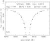 |
Fig. 4 Fitting of the computed to the observed fluxes of the solar Hα profile. Open circles are the theoretical profile, the red ones corresponding to the wavelength of the observed points represented by full black stars. |
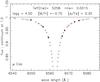 |
Fig. 5 Fitting of the computed to the observed fluxes on the Hα profile of μ Cas, same symbols as in Fig. 4. |
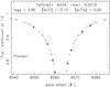 |
Fig. 6 Fitting of the computed to the observed fluxes on the Hα profile of Procyon. |
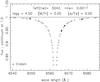 |
Fig. 7 Fitting of the computed to the observed fluxes on the Hα profile of ϵ Eridani. |
3. Effective temperatures from the direct method
3.1. The apparent diameters
The direct method could not be applied before a significant number of accurate apparent angular diameters were obtained by interferometric measurements. Thanks to continuous improvements in Mount Wilson interferometer MARKIII (Mozurkewich et al. 2003), now CHARA interferometer (Baines et al. 2008, and other references therein) and more recently to VLTI new determinations (Kervella & Fouqué 2008), ten unevolved stars have apparent diameters known with a relative accuracy of higher than 2 percent, contributing by less than 1 per cent to the accuracy of Teff obtained by Eq. (1). Each of the ten stars have an effective temperature derived from Hα (here after Teff(Hα) and another one derived from the direct method (here after Teff(direct). These ten stars, in addition to the Sun, are our calibrating objects for the relation Teff(Hα) versus Teff(direct).
3.2. The determination of bolometric fluxes
Although bolometric flux appears in Eq. (1) with the power 1/4, it is necessary to keep the relative error in fbol lower than 2 percent so as not to degrade the superb accuracy of the apparent diameters. Fortunately, the analysis presented by Casagrande et al. (2010) allows us to solve this problem. It contains a table allowing us to derive apparent bolometric fluxes from different photometric bands, as a function of various colour indices (their Table 5). We converted the J magnitudes into bolometric fluxes using the V − J index, and the Ks magnitudes into bolometric fluxes using the V − Ks index. The one sigma deviation of the fbol(J) is 0.8 percent for a sample of 300 stars, and 1.1 percent for the fbol(Ks). A slight difficulty is that all the calibration stars are too bright for the 2MASS survey. We were therefore obliged to use Johnsson J and K magnitudes, and convert them into J and Ks of the 2MASS system. To achieve this we used the transformation formulae given in the 2MASS Explanatory Supplement4 (2)and
  (3)We then averaged the two fbol(J) and fbol(Ks) as our own estimate. Independently, Casagrande et al. used the colours B, V, RCousins, and ICousins to obtain the bolometric fluxes. Table 1 shows the two determinations, which are in good agreement in spite of their being derived from two entirely different colour sets. We adopted the arithmetic mean of the Casagrande fbol1 and our fbol2 as the final estimate of the bolometric fluxes.
Effective temperatures from both Hα and the direct method.
4. The connection between the effective temperatures derived from Hα and the direct method
For each object, Table 2 contains the two effective temperatures and additional informations about the calibrating stars. We recall that Teff(direct) is assumed to represent the true effective temperature of the star, whereas Teff(Hα) represents the effective temperature of the model atmosphere that provides the closest fit of the Hα profile of the spectrum of the star. With perfect models, the two temperatures would be equal. As the effective temperature reflects a property of the full atmosphere, and Teff(Hα) a property of a rather limited portion of this atmosphere, it is understandable that some difference may exist. The question is of course whether there is a well defined relation between both determinations, or not. Figure 8 shows the linear regression between the two temperatures. The rms of Teff(direct) versus the regression line is only 30 K, which is a very small scatter. The correlation coefficient between the two sets of temperatures is 0.9976 which represents an extremely tight link. The equation of the regression line is  (4)This simple relation enables us to convert Teff(Hα) into Teff(direct), which was the aim of this paper. More accurately, it is useful to know the balance-sheet of the various sources of errors involved in the transformation of Teff(Hα) into Teff(direct). Table 3 gives the full set of the uncertainties, and the resulting total uncertainty induced in the derived Teff. The 0.1 uncertainties in log g, [M/H], and [Fe/H] are only examples, which must be adjusted to each particular case.
5. The case of metal-poor stars
In our sample, the most metal-poor star is μ Cas (not a halo star but rather a thick disk star) with [Fe/H] = −0.7. The model atmosphere of a real halo star, with a metallicity in the range from − 1.5 to − 3., has drastic structural differences in continuous opacity and blanketing effect with respect to the stars of our calibration. We cannot expect Eq. (4) to apply to them. There are presently only two stars with an accurately measured angular diameter i.e. HD 122563 (a giant) and HD 103095 (a cool dwarf), so the present sample is very small. There is a serious hope that in a few years the situation will improve, and that the direct method can then be used. For the moment, we have to use the second best method, the infrared flux method (IRFM), introduced by Blackwell & Shallis (1977), which is more model dependent than the direct method. Several implementations of the IRFM have been developed over the years. The first one applied to a sample rich in metal-poor stars was that of Alonso et al. (1996). Other implementations supported different effective temperature scales, with departures exceeding 200 K for very metal-poor stars (Ramirez & Melendez 2005). A detailed discussion of these differences is available in Casagrande et al. (2010). Fortunately, recent implementations of the IRFM, Gonzalez Hernandez & Bonifacio (2009) and Casagrande et al., both using the 2MASS photometric catalogue5, have been in much closer agreement, with a mean offset of 30 to 40 K between the two scales. Before more accurate angular diameter become available we recommend using these last two implementations to detemine the effective temperatures. If these stars are too bright for the 2MASS catalogue, a transformation of other colours to the 2MASS system may be necessary, as performed by ourselves.
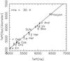 |
Fig. 8 Regression line between Teff(Hα) and Teff(direct), represented by Eq. (4), has an rms of 30 K. |
List of the errors induced by various sources.
6. Discussion
The improved accuracy of the broadening theories of the Balmer Hα line has allowed us to establish a solid empirical calibration of the observed profiles of the line into effective temperatures, in the ranges of Teff from 5000 K to 6600 K, of [Fe/H] from − 0.8 to 0.20, and of log (g) from 4.5 to 4.0, corresponding to a range from dwarf to subgiant stars. However, this calibration shows that the obtained effective temperatures are not equal to the effective temperatures of the models producing the best fit, but about 100 K higher. The origin of the discrepancy is likely that the region of formation of Hα is rather special, a narrow part of the radiative zone above the convective zone, whereas the effective temperature probes the whole atmosphere.
For the Sun, we have not only theoretical model atmospheres, but empirical models, such as the Harvard models (Fontenla et al. 1993). Figure 9 shows the observed and computed profiles of Hα for the Kurucz solar theoretical model and the empirical FAL93 model. Both models fail to reproduce the observations but produce significantly different profiles. Figure 10 shows the difference between stratification of the Kurucz and the FAL93 solar models. The two depart strongly above their crossing point, at the mass depth of 5.0 g/cm2, in the region of Hα line formation. It is not the role of 1D models to resolve this inconsistency, as it has already been shown that in 3D radiative hydrodynamical models horizontal temperature fluctuations play an important role in producing the Balmer line profiles (Ludwig et al. 2009). In this reference, we note that a 3D model supplying an Hα profile similar to that obtained with a 1D model (with our l/Hp = 0.5) has an effective temperature 34 K higher than the 1D model, for atmospheric parameters close to those of the Sun, and we refer to Behera et al. (2009). We are presently preparing a second paper re-investigating the same sample of stars with 3D models.
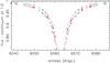 |
Fig. 9 Hα profiles. Red symbols correspond to the eight observed windows. Stars: observed profile points, circles: computed points from solar Kurucz’s model, squares: computed points from FAL93 empirical model. Both computed profiles fail to reproduce the observed profile. Kurucz profile fits the far wings, FAL93 fits the region 4 to 6 Å from the line center. |
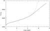 |
Fig. 10 The ATLAS9 solar model (dotted line) and the FAL93 empirical one (full line). The crossing point near mass depth = 5.0 has an optical depth τRoss = 2. |
7. Conclusions and future work
We present our main findings in this paper and plan for future work:
-
1.
Using up-to-date theories of the Hα broadening mechanisms, we have been able to obtain excellent fits of observed stellar Hα profiles with computed ones, using 1D Kurucz Atlas9 models, in the temperature range from 5000 K to 7000 K, the other parameters metallicity, [α/Fe] , and log g being fixed by a reliable detailed analysis of the atmosphere.
-
2.
However, the best fit is obtained for an effective temperature of the model that differs from the true effective temperature of the star, obtained with the fundamental method, using the apparent bolometric flux and the apparent angular diameter of the star.
-
3.
Fortunately, the two sets of effective temperatures are highly correlated. This enabled us to propose a simple linear relationship to transform the temperature derived from the Hα profile into the true effective temperature of a star, which is the essential result of this paper.
-
4.
The new values of the collisional self-broadening of Hα have raised a problem that had remained hidden for over 30 years, because of the far too small value of the cross-section proposed by Ali-Griem which had been largely used since 1966. The accuracy of the new values excludes the former agreement between observed and computed Hα profiles with 1D models. The comparison of the solar temperature stratification in both theoretical and empirical models leaves room for an uncertainty of the order of 100 K in the region of formation of the line, in layers just above the convective zone. Only 3D radiative hydrodynamical models, relying on fundamental physics are adequate to model the complex situation there. Former published works provided encouraging results. A forthcoming paper will reconsider our calibration with 3D models.
Available at http://www.ipac.caltech.edu/2mass
Acknowledgments
Many thanks to R. Kurucz for allowing the use of his ATLAS9 and BALMER9 codes and his opacity data. We are indebted to L. Casagrande for supplying us the bolometric fluxes used in Casagrande et al. (2010), and for several useful advices. We are indebted to P. Kervella for making available to us his expertise in the field of angular diameter measurements. We also thank D. Katz for making available his script for the exploitation of the ATLAS9 code, M. Steffen for helpful comments, and P. Bonifacio and E. Caffau for their continuous support during the course of this work.
References
- Ali, A. W., & Griem, H. R. 1966, Phys. Rev. A, 144, 366 [NASA ADS] [CrossRef] [Google Scholar]
- Allard, N. F., Kielkopf, J. F., Cayrel, R., & van ’t Veer-Menneret, C. 2008, A&A, 480, 581 [NASA ADS] [CrossRef] [EDP Sciences] [Google Scholar]
- Allen de Prieto, C., Barklem, P. S., Lambert, D. L., & Cunha, K. 2004, A&A, 420, 183 (S4N) [NASA ADS] [CrossRef] [EDP Sciences] [Google Scholar]
- Alonso, A., Arribas, S., & Martínez-Roger, C. 1996, A&AS, 117, 227 [NASA ADS] [CrossRef] [EDP Sciences] [Google Scholar]
- Baines, E. K., McAlister, H. A., ten Brummelaar, T. A., et al. 2008, ApJ, 680, 728 [NASA ADS] [CrossRef] [Google Scholar]
- Barklem, P. S., Piskunov, N., & O’Mara, B. J. 2000, A&A, 362, 1091 [NASA ADS] [Google Scholar]
- Barklem, P. S., Stempels, H. C., Allen de Prieto, C., et al. 2002, A&A, 385, 951 [NASA ADS] [CrossRef] [EDP Sciences] [Google Scholar]
- Behara, N. T., & Ludwig, H.-G. 2009, Cool Stars, stellar systems and the Sun, AIP Conf. Proc., 1094, 784 [Google Scholar]
- Blackwell, D. E., & Shallis, M. J. 1977, MNRAS, 180, 177 [NASA ADS] [CrossRef] [Google Scholar]
- Böhm-Vitense, E. 1958, ZAp, 46, 108 [NASA ADS] [Google Scholar]
- Boyajian, T. S., McAlister, H. A., Baines, E. K., et al. 2008, ApJ, 683, 424 [NASA ADS] [CrossRef] [Google Scholar]
- Bonifacio, P., Molaro, P., Sivarani, T., et al. 2007, A&A, 462, 851 [NASA ADS] [CrossRef] [EDP Sciences] [Google Scholar]
- Brissaud, A., & Frisch, U. 1971, JQRST, 11, 1767 [Google Scholar]
- Casagrande, L., Ramírez, I., Meléndez, J., et al. 2010, A&A, 512, A54 [NASA ADS] [CrossRef] [EDP Sciences] [Google Scholar]
- Fontenla, J. M., Avrett, E. H., & Loeser, R. 1993, ApJ, 406, 319 [NASA ADS] [CrossRef] [Google Scholar]
- Fuhrmann, K., Axer, M., & Gehren, T. 1993, A&A, 271, 451 [NASA ADS] [Google Scholar]
- Fuhrmann, K., Pfeiffer, M., Franck, C., Reetz, J., & Gehren, T. 1997, A&A, 323, 909 [NASA ADS] [Google Scholar]
- Gehren, T., Shi, G. R., Zhang, H. W., Zhao, G., & Korn, A. J. 2006, A&A, 451, 1065 [NASA ADS] [CrossRef] [EDP Sciences] [Google Scholar]
- González Hernández, J. I., & Bonifacio, P. 2009, A&A, 497, 497 [NASA ADS] [CrossRef] [EDP Sciences] [Google Scholar]
- Gratton, R., Bonifacio, P., Bragaglia, A., et al. 2001, A&A, 369, 87 [NASA ADS] [CrossRef] [EDP Sciences] [Google Scholar]
- Heiter, U., Kupka, F., van ’t Veer-Menneret, C., et al. 2002, A&A, 392, 619 [NASA ADS] [CrossRef] [EDP Sciences] [Google Scholar]
- Henyey, L., Vardya, M. S., & Bodenheimer, P. 1965, ApJ, 142, 841 [NASA ADS] [CrossRef] [Google Scholar]
- Holweger, H., & Müller, E. A. 1974, Sol. Phys., 39, 19 [NASA ADS] [CrossRef] [Google Scholar]
- Kervella, P., & Fouqué, P. 2008, A&A, 491, 855 [NASA ADS] [CrossRef] [EDP Sciences] [Google Scholar]
- Kurucz, R. L. 2OO5, http://kurucz.harvard.edu/sun [Google Scholar]
- Ludwig, H.-G., Behara, N. T., Steffen, M., & Bonifacio, P. 2009, A&A, 502, L1 [NASA ADS] [CrossRef] [EDP Sciences] [MathSciNet] [Google Scholar]
- Mashonkina, L., Zaho, G., Gehren, T., et al. 2008, A&A, 478, 529 [NASA ADS] [CrossRef] [EDP Sciences] [Google Scholar]
- Mozurkewich, D., Armstrong, J. T., Hinsley, R. B., et al. 2003, AJ, 126, 2502 [NASA ADS] [CrossRef] [Google Scholar]
- North, J. R., Davis, J., Robertson, J. G., et al. 2009, MNRAS, 393, 245 [NASA ADS] [CrossRef] [Google Scholar]
- Ramírez, I., & Meléndez, J. 2005, ApJ, 626, 446 [Google Scholar]
- Soubiran, C., Le Campion, J.-F., Cayrel de Strobel, G., & Caillo, A. 2010, A&A, 515, A111 [NASA ADS] [CrossRef] [EDP Sciences] [Google Scholar]
- Spielfiedel, A., Palmieri, P., & Mitrushenkov, A. O. 2004, Molec. Phys., 102, 2249 [NASA ADS] [CrossRef] [Google Scholar]
- Stehlé, C., & Hutcheon, R. 1999, A&AS, 140, 93 [NASA ADS] [CrossRef] [EDP Sciences] [Google Scholar]
- van Belle, G. T., Ciardi, D. R., & Boden, A. F. 2007, ApJ, 657, 1058 [NASA ADS] [CrossRef] [Google Scholar]
- Vidal, C. R., Cooper, J., & Smith, E. W. 1973, ApJS, 25, 37 [NASA ADS] [CrossRef] [Google Scholar]
All Tables
All Figures
|
Fig. 1 Windows, delimitated by green vertical lines, and telluric lines, indicated by red arrows, on the blue wing of the observed solar Hα profile. |
| In the text | |
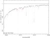 |
Fig. 2 Same as Fig. 1, except that it is for the red wing of Hα. |
| In the text | |
|
Fig. 3 Same as Fig. 1, but for the observed blue wing of Hα on the μ Cas spectrum. Clearly the bluest window (6549.50 Å) is entirely lost, because obliterated by a telluric line. |
| In the text | |
|
Fig. 4 Fitting of the computed to the observed fluxes of the solar Hα profile. Open circles are the theoretical profile, the red ones corresponding to the wavelength of the observed points represented by full black stars. |
| In the text | |
|
Fig. 5 Fitting of the computed to the observed fluxes on the Hα profile of μ Cas, same symbols as in Fig. 4. |
| In the text | |
|
Fig. 6 Fitting of the computed to the observed fluxes on the Hα profile of Procyon. |
| In the text | |
|
Fig. 7 Fitting of the computed to the observed fluxes on the Hα profile of ϵ Eridani. |
| In the text | |
|
Fig. 8 Regression line between Teff(Hα) and Teff(direct), represented by Eq. (4), has an rms of 30 K. |
| In the text | |
|
Fig. 9 Hα profiles. Red symbols correspond to the eight observed windows. Stars: observed profile points, circles: computed points from solar Kurucz’s model, squares: computed points from FAL93 empirical model. Both computed profiles fail to reproduce the observed profile. Kurucz profile fits the far wings, FAL93 fits the region 4 to 6 Å from the line center. |
| In the text | |
|
Fig. 10 The ATLAS9 solar model (dotted line) and the FAL93 empirical one (full line). The crossing point near mass depth = 5.0 has an optical depth τRoss = 2. |
| In the text | |
Current usage metrics show cumulative count of Article Views (full-text article views including HTML views, PDF and ePub downloads, according to the available data) and Abstracts Views on Vision4Press platform.
Data correspond to usage on the plateform after 2015. The current usage metrics is available 48-96 hours after online publication and is updated daily on week days.
Initial download of the metrics may take a while.