© ESO, 2011

1. Introduction

The mechanism responsible for the initiation of solar flares attracts attention in the context of the flare forecasting (e.g. Schrijver 2009) as well as of the understanding of quasi-periodic pulsations in flares (Nakariakov & Melnikov 2009) and the phenomenon of the sympathetic flares (Moon et al. 2002; Akimov et al. 2008). In particular, there is some observational evidence that the triggering of a flare can be associated with magnetohydrodynamic (MHD) waves and oscillations. Foullon et al. (2005) demonstrated that long-period pulsations of flaring emission can be associated with MHD oscillations of a large, trans-equatorial coronal loop. Sych et al. (2009) found that propagating slow magnetoacoustic waves could trigger flaring energy releases.

The specific mechanism for the triggering of magnetic reconnection by MHD waves has not been established yet, however, several possibilities have been identified. Chen & Priest (2006) proposed that slow magnetoacoustic waves can induce magnetic reconnection by modulating the density of the plasma in the vicinity of the reconnection site. Nakariakov et al. (2006) developed a model of the triggering of magnetic reconnection by fast magnetoacoustic waves. In this model, fast waves generate steep spikes of the electric current density in the vicinity of a magnetic null point, which drive plasma micro-instabilities and, hence, the anomalous resistivity.

Various models for the interaction of MHD waves with magnetic null points have been put forward. For example, Craig & McClymont (1991) considered a magnetoacoustic m = 0 mode disturbing an equilibrium 2D null-point. They took into account the magnetic diffusivity and showed that the decay of the m = 0 oscillations on the null-point is limited by the dissipation time-scale of the fundamental mode with no dependency on the number of radial nodes. The magnetic reconnection was found to show oscillatory dynamics. It was deduced that oscillatory reconnection was caused by the dissipation of free magnetic energy. Furthermore, waves in the neighborhood of a 2D null point have been investigated by Craig & Watson (1992). They considered the radial propagation of the m = 0 mode in the zero-β regime and stated that reconnection could only take place if the disturbances are purely radial. They also confirmed that the reconnection is oscillatory and fast with a logarithmic dependency on magnetic resistivity η.

McLaughlin & Hood (2004) considered the behaviour of a single 2D fast magnetoacoustic wave-pulse approaching a null point in the zero-β regime. The authors showed that the wave-pulse never exactly reaches the null point in this model, because the Alfvén wave looses the speed the closer it approaches the null point. Due to refraction, the wave-pulse bends around the null-point, creating a density spike. More recently, McLaughlin & Hood (2006) extended their model to the finite-β regime and noticed coupling between slow and fast magnetoacoustic waves and mode conversion at locations where the sound and Alfvén speeds are comparable. Similar effects were studied by Zhugzhda & Dzhalilov (1982) and Cally (2001) in the context of the wave energy transport in an isothermal magnetised atmosphere.

Longcope & Priest (2007) studied the resistive dissipation of a 2D current sheet above a null-point caused by anomalous resistivity. They used cartesian geometry to describe a planar equilibrium magnetic field for the null-point and a 2D current sheet that was placed in the equilibrium magnetic field. They deduced that owing to the disruption of the current sheet by diffusion, outgoing fast magnetoacoustic waves could be launched by null-point reconnection. The recent study of McLaughlin et al. (2009) extended their previous investigations by taking into account nonlinear effects, studying the formation of magnetoacoustic shocks in the vicinity of a null point.

The aim of this paper is to develop the work of McLaughlin et al. (2009), performing the parametric study of the nonlinear steepening of a fast magnetoacoustic wave near a null point. First, we re-examine and confirm the results of McLaughlin et al. (2009), and interprete it in terms of nonlinear MHD wave theory. Then, we study the departure from the linear solution of Craig & McClymont (1991) caused by the nonlinearity. We calculate the distance of magnetoacoustic shock formation from the null point as a function of initial wave-pulse length and amplitude. This clarifies what kind of pulses can reach the magnetic null point and create a spike of the current density close to the null point, initiating magnetic reconnection.

This paper is organized as follows. The analytical model is considered in Sect. 2. Numerical simulations are described in Sects. 3.1 and 3.2. Numerical results are presented and discussed in Sect. 3.4. This paper is concluded by a summary of the main results in Sect. 4.

2. Analytical description

2.1. Model and equilibrium conditions

Ideal MHD equations for typical coronal conditions in the low-β regime are considered using the cylindrical coordinate system (r,ϕ,z) 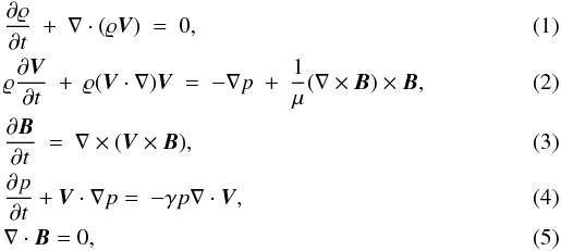where ϱ is the mass density, p is the gas pressure, B is the magnetic field, V is the flow velocity, μ is the magnetic permeability and γ = 5/3 is the ratio of specific heats. The equilibrium is considered identical to that described in McLaughlin et al. (2009)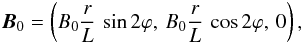(6)where L is a characteristic length scale, r is the radial distance from the null-point and ϕ is the azimuthal angle (Fig. 1). The characteristic length L is connected with the width of the wave-pulse or its initial position. We also consider the gas pressure, density and temperature to be constant everywhere. In this equilibrium, the radial dependence of the Alfvén speed is independent of the polar angle, 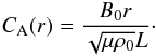(7)Linearising the MHD equations with respect to the equilibrium and considering no azimuthal dependency (∂/∂ϕ = 0) and also no dependency on the z coordinate perpendicular to the plane of the null-point (∂/∂z = 0), we obtain 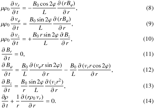Combining Eqs. (9) and (12) we get 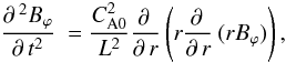(15)where C_A0 is the background Alfvén speed measured at r = L, C_A0 = C_A(r = L).

By defining 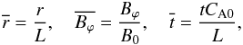(16)we have the normalised form of Eq. (15) as 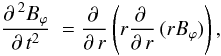(17)where we have omitted the overline. The solution for the perturbations of the azimuthal magnetic field is 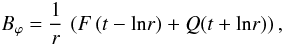(18)where functions F and Q describe the shape of the inwardly and outwardly propagating waves respectively, Craig & McClymont (1991). Because we are considering the magnetoacoustic wave propagating towards the null-point, we are only interested in the first term of expression (18) which shows the incoming wave. Because we work in the zero-β approximation, this model is applicable at some distance from the null-point only, far from the radius of β being a unity. Obviously, the perturbations of the magnetic field propagate independently of the polar angle ϕ. Combining Eqs. (8) and (18) and normalising the radial velocity as where we again omit the overtilde, we obtain the normalised radial velocity in the inwardly propagating wave, 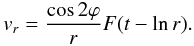(19)Below we compare this solution in Sect. 3.4 with the results of numerical simulations for different wave amplitudes, showing its time evolution as the wave approaches the null point.

2.2. Weakly nonlinear effects

Consider weakly-nonlinear fast waves approaching the null-point. Restricting ourselves to the analysis of the quadratically nonlinear effects only, and following the formalism developed in Nakariakov et al. (2000), we obtain 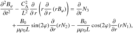(20)where N₁, N₂ and N₅ are the quadratically nonlinear terms on the right-hand sides of Eqs. (8), (9) and (12), respectively. The expressions for the nonlinear terms are 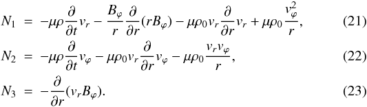We change the frame of reference using the linear solution (18) 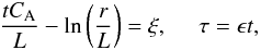(24)where ϵ is a small parameter that represents the smallness of the nonlinear terms in Eq. (20). Hence, τ is a “slow” time, representing the slow evolution of the linear solution because of the weak nonlinearity. Equation (20) in the new frame of reference becomes 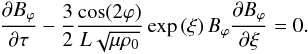(25)This equation is of the Burgers type, without the dissipative term. In general, it describes nonlinear acceleration and steepening of the wave-pulse because of the nonlinearity. In a uniform medium, steeper wave-pulses of higher amplitude are known to form shocks quicker. We observe that the coefficient in the second, nonlinear term of Eq. (25) depends on the azimuthal angle ϕ. This means that the nonlinear evolution of the initially axisymmetric pulse is different in different polar angle directions. The highest value of the nonlinear coefficient is for the angles, where the equilibrium magnetic field is perpendicular to the radial vectors. The coefficient becomes zero in the directions of the magnetic separatrices of the equilibrium. This is because in this directions the wave vector is parallel to the magnetic field, and the fast waves degenerate to the Alfvén waves. Alfvén waves are not subject to the quadratic nonlinearity (e.g., Nakariakov et al. 2000). The dependence of the nonlinear coefficient on the azimuthal angle makes further analytical treatment impossible, because Eq. (25) was derived under the assumption of the independence of the angle perturbations. However, Eq. (25) gives us the important qualitative information about the azimuthal dependence of the fast wave evolution, which can be used for the understanding of numerical results.

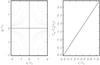Fig. 1 Null-point configuration showing the equilibrium magnetic field lines (curved lines) and the separatrices (red lines) that separate the configuration into four quarters (left panel). The Alfvén speed dependence on the distance to the null-point (right panel). The parameters are normalised by the distance of the initial pulse to the null-point (r1).

3. Numerical simulations

3.1. Numerical methods

Magnetohydrodynamic Eqs. (1)–(5) are solved numerically using the Lagrangian-remap code, Lare2d (Arber et al. 2001). Lare2d operates by taking a Lagrangian predictor-corrector time step, after each Lagrangian step all variables are conservatively re-mapped back onto the original Eulerian grid using Van Leer gradient limiters. The code was designed for the simulation of nonlinear dynamics of low β plasmas with steep gradients and accordingly, suits the problem of interest very well.

The magnetic field B is defined on cell faces and is updated with a constrained transport to keep ∇·B = 0 to machine precision. We simulated the plasma dynamics in a domain (0,10) × (0,10) Mm covered by 3000 × 3000 grid points. We performed grid convergence studies to check the numerical results. Zero gradient boundary conditions were set for all simulations. We observed little reflection from boundaries, but during our numerical studies we considered only the initial value problem, studying the evolution of the pulses that propagate towards the X-point. We stopped our simulations when the inwardly propagation pulse overturned. Our simulation region was large enough and our numerical results were not affected by reflection from the boundaries.

3.2. Initial setup

Our initial state is a simple 2D magnetic null-point with a fast magnetoacoustic pulse on the (x,y) plane initialised at some distance from the null-point. Our choice of the equilibrium magnetic field is (26)where B₀ is the strength of the magnetic field and L is a characteristic length scale. The configuration of the magnetic field lines is illustrated in Fig. 1. The initial fast magnetoacoustic pulse is circular with the centre at the origin, as in McLaughlin et al. (2009), and is initiated in the ring region 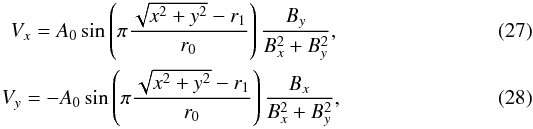where the amplitude was taken to be A₀. The specific quantitative values of the initial equilibrium are taken to be consistent with the typical parameters of the solar coronal plasma (see Table 1). In the following, the typical values of the initial pulse were r₁ = 5 Mm, r₀ = 1 Mm and A₀ = 10³ m/s.

This set-up of the numerical experiment is similar to the one of McLaughlin et al. (2009). Likewise, the development of the initial pulse observed in out study, is similar to the scenario described in McLaughlin et al. (2009). As time progresses, the initially axisymmetric and static pulse is observed to develop into two pulses, one propagating inwards and the other outwards. The inward pulse experiences numerical steepening and acceleration or deceleration. The segments of the inward pulse, propagating in different quadrangles of the coordinate system, are either accelerated or decelerated, and the shocks are formed at either front or back slopes.

3.3. Local phase relations in magnetoacoustic modes

For the interpretation of numerical results, it is instructive to consider fast magnetoacoustic waves propagating in a uniform medium penetrated by a straight and uniform magnetic field. Consider the equilibrium magnetic field in the z-direction B_z0 and a wave propagating in the x-direction with no dependencies on other components (∂/∂y = 0,∂/∂z = 0) in the zero-β limit. This coordinate system is different from the one used in Sect. 2, and can be considered as a local coordinate system where the magnetic field is locally perpendicular to the radial vector.

The linearised MHD equations around the equilibrium are Applying the Fourier decomposition (∂/∂x = ik,∂/∂t = iω) of the expressions in Eq. (29), we obtain (31)and (32)Equations (31) and (32) are the relations between the perturbations of different physical quantities, which show that the perturbations are related to each other by the phase speed (which in the considered case is the Alfvén speed C_A0, and can be positive or negative). Therefore the direction of the wave propagation would affect the phase relations between the perturbations of the density and velocity.

To illustrate this, it is worth discussing the results of McLaughlin et al. (2009), where a fast magnetoacoustic pulse was set to run towards the null-point. The results of the simulation are shown in Fig. 2. The top left and middle panels show the v_x and v_y profiles respectively, and the top right panel shows the initial density perturbation that is uniform at t = 0 s. The arrows show the direction of the initial velocity profile and the blue and red colours indicate the negative and positive signs, respectively. The opposite signs of the perturbations are showing their effects in the bottom row, each panel shows the ingoing and outgoing pulses at t = 8 s where the radial shape of the pulse and density perturbation has been deformed to an elliptical shape by the nonlinearity.

This behaviour can be explained with the use of the local approach described above. From the phase relations (31) and (32), which show the dependency of the density perturbation in the direction of the velocity, the density perturbation is anti-phase in quarters 1 and 3 compared to quarters 2 and 4. Hence, the density perturbation has an azimuthal dependency and is not propagating with the azimuthal wave number m = 0, which is a symmetric mode. Therefore, a nonlinear, initially symmetric wave-pulse shows the development of the asymmetry of the density perturbation. This asymmetry explains the front (compression pulse) and backward (rarefaction pulse) overturning of the wave-pulse, seen in McLaughlin et al. (2009) and in Fig. 2. Accordingly, an initially axisymmetric, m = 0 perturbation, in the nonlinear regime, becomes dependent on the polar angle, and departs from the m = 0 symmetry.

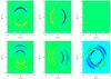Fig. 2 Top row, contours of the parameters vx, vy, and ρ at t = 0 s and bottom row, the corresponding parameters at t = 0.8 s. The arrows on the top left figure show the initial velocity profile. The red and blue colours indicate positive and negative signs respectively. In the bottom row the ingoing and outgoing pulses could be seen.

3.4. Parametric studies

3.4.1. Compression pulse

We performed a series of numerical experiments to study the generation of fast magnetoacoustic shocks in the vicinity of a null-point. First we investigated a compression pulse. Figure 3 shows contour plots of velocity at four different instants of time. We show only first quarter of simulation region (x > 0,   y > 0). The white curve shows the position of the linear solution. It is clearly visible and we illustrated in Sect. 3.3 that the pulse shape changes from circular to an elliptical-like shape, because of the dependence of the nonlinear coefficient upon the azimuthal angle.

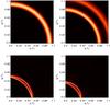Fig. 3 Two-dimensional plots of the absolute values of the radial velocity at t = 0 s (top left panel), t = 0.4 s, (top right panel), t = 1.6 s, (bottom left panel), and t = 2.4 s (bottom right panel). White curves show the linear solution. The spatial coordinates are measured in units of r1, which is the initial position of the fast wave-pulse.

Figure 4 demonstrates the consistency of the numerical results, because they reproduce the analytical solution given by Eq. (19). It also shows the departure of the nonlinear results from the linear solution, because the wave amplitude grows. This means that the pulse speed towards the null-point is proportional to the wave initial amplitude, with higher amplitude pulses having higher speeds. Clearly, our simulations are valid only before the shock is formed, because then the dissipative effects become decisive and must be taken into account.

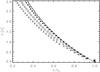Fig. 4 Comparison of numerical results simulating incoming fast magnetoacoustic pulses of different amplitude with the analytical solution of Eq. (19). The solid line (points) corresponds to the analytical (numerical) solution. The amplitude of the initial pulse was A0 for the triangles, 0.5A0 for the squares, 0.1A0 for the stars and 0.01A0 for the crosses. The spatial coordinate is measured in units of r1.

Figure 5 displays the radial velocity of the pulse measured for the azimuthal angle corresponding to the propagation perpendicular to magnetic filed lines, (33)versus the radius r at three instants of time. The blue and red profiles correspond to two different amplitudes. This considered pulse is the pulse of compression, therefore the radial velocity perturbation is directed inwards, in the same direction as the wave vector. In the polar frame of reference, this flow would be negative, hence we show its absolute value. Obviously the higher amplitude pulse “overturns” – forms the shock – faster than the smaller amplitude pulse. In addition, the radial velocity is accompanied by current density spikes (McLaughlin et al. 2004, 2006, 2009) as the wave amplitude increases in time, which gives rise to anomalous resistivity. This is shown in the three snapshots of Fig. 6.

Fig. 5 Perturbations of the absolute value of the radial velocity in the inwardly propagating pulse of compression, as a function of the radial position r. Different colours (thickness) correspond to two different initial amplitudes of the pulse. The red (thick) curves correspond to the instants of time t = 0.3 s (solid), t = 0.5 s (dotted), and t = 0.7 s (dashed). The blue (thin) curves correspond to t = 0.5 s (solid), t = 0.8 s (dotted), and t = 1.1 s (dashed). The spatial coordinate is measured in units of r1.

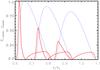Fig. 6 Generation of the electric current density spikes in a fast magnetoacoustic pulse. Perturbations of the absolute value of the radial velocity in the inwardly propagating pulse of compression, , are shown as a function of the radial coordinate r by the blue (thin) curves. The spikes of electric current density are shown by the red (thick) curves. The snapshots of the pulses (from right to left) correspond to the instants of time t = 0.5 s, t = 0.8 s and t = 1.1 s. The parameters are normalised by the maximum values at t = 1.4 s. The radial coordinate is measured in units of r1.

In order to estimate the position of the shock formation, we observed the shock’s evolution. When the amplitude of the pulse decrease, we assume that the shock appears. Because the gradient in a narrow pulse is higher than for a wider pulse, the shock should be created faster. In the astrophysical and geophysical literature, the effect of the generation of anomalous resistivity in the regions with the high current density has been studied in great detail (see, e.g. Büchner & Elkina 2005; Petkaki et al. 2006). We emphasise that the anomalous resistivity is generated before the fast wave pulse forms a shock, because the necessary condition for the onset of the current-driven instabilities is that the current density exceeds some certain (finite) threshold value (e.g., Yokoyama & Shibata 1994; Nakariakov et al. 2006, for the discussion of this effect in the solar flare context).

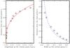Fig. 7 Distance from the null-point to the position of the fast shock formation as a function of the amplitude of initial pulse (left panel) and width of initial pulse (right panel). The solid curves show the best-fitting exponential functions. Spatial coordinates and amplitude are measured in units of r1 and Alfvén speed CA(r1).

Figure 7 illustrates the dependence of the shock formation distance from the null-point on the amplitude and the initial width of the pulse. The left panel shows the shock generation for different amplitudes of the initial pulse all other parameters of the run are fixed. The right panel shows the shock generation with respect to the initial width of the pulse. The spatial coordinates are normalised by the initial distance of the pulse from the null-point r₁, and the velocity amplitude is normalised by the local Alfvén speed. Evidently, higher amplitude pulses generate shocks further away from the null-point, while pulses with larger width form the shock closer to the null-point. In a uniform medium the distance of the shock formation depends on the wave length λ and an amplitude A as (34)where d is a distance from null point. In our studies we considered a non-uniform magnetic field and the above relation should be more complicated. Applying the least-squares approximation method, we determine the empirical dependence d ~ A^0.32/λ^0.46 (Fig. 7 red (solid) and blue (dashed) lines).

3.4.2. Rarefaction pulse

We now investigate the pulse of the rarefaction. As expected, this pulse is nonlinearly decelerated, in contrast with the compression pulse (McLaughlin et al. 2009). Figure 8 displays the profiles of the radial velocity v_r in the rarefaction pulse versus the radial coordinate r at three instants of time. The blue (thin) and red (thick) profiles correspond to two different initial amplitudes. Obviously, that the rarefaction pulse “overturns” at the back slope. Similar to the compression pulse, the higher amplitude pulse “overturns” faster than the smaller amplitude pulse (Fig. 8). From the three snapshots of Fig. 9 we can see that the current density spikes appear at the back slope of the pulse.

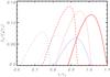Fig. 8 Snapshots of the radial velocity in the inwardly propagating pulse of rarefaction, as a function of the radial coordinate r. Different colours and thickness correspond to two different initial amplitudes of the pulse. Red (thick) line corresponds to the instants of time t = 0.3 s (solid), t = 0.5 s (dotted), t = 0.7 s (dashed), and blue (thin) to t = 0.5 s (solid), t = 0.8 s (dotted), and t = 1.1 s (dashed). The radial coordinate is measured in units of r1.

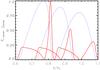Fig. 9 Perturbations of the radial velocity in the inwardly propagating pulse, as a function of the radial position r. The spikes (red thick spikes) correspond to the current density j and the blue thin curves correspond to vr at times t = 0.5 s, t = 0.8 s, t = 1.1 s. The parameters are normalised by the maximum values of vr and t at t = 1.4 s, and the radial coordinate is measured in units of r1.

4. Summary and discussion

We have performed an analytical study accompanied by numerical simulations of the behaviour of a fast magnetoacoustic pulse approaching a null-point. Using ideal MHD equations in the zero-β regime (hence, at some sufficiently large distance from the radius β = 1), we developed a 1D analytical model of an initially axisymmetric m = 0 fast pulse in the weakly nonlinear regime. We derived the evolutionary equations for the radial velocity of the pulse, and showed that the evolution of the pulse leads to a departure from the azimuthally symmetric m = 0 mode, but is rather of the symmetry of the m = 2 mode or higher. Consideration of the excitation conditions and of the phase relations in the numerical experiments of McLaughlin et al. (2009) supported that observation. Numerical simulations of the nonlinear development of an initially Gaussian pulse of a finite amplitude, confirmed the azimuthal dependency of the fast magnetoacoustic pulse for a quarter of a circle, justifying our analytical explanation for the pulse evolution. We also showed in our simulation that small amplitudes pulses coincide with the linear analytical solution of Craig & McClymont (1991).

We showed that the pulses of the plasma compression of higher initial amplitudes propagate faster. In contrast with that, pulses of rarefaction experience deceleration with the increase in the amplitude. Moreover, our numerical studies showed that similarly to the case of a uniform medium, the position and time of the pulse overturning is also determined by its initial steepness (connected with its initial width). Thus, initially lower amplitude and broader fast-wave pulses form fast shocks – “overturn” – closer to the null-point. Because the shock formation is accompanied by the generation of electric current density spikes, in the vicinity of the shock formation region we can expect the onset of plasma micro-turbulence, and hence the appearance of anomalous electrical resistivity.

Our finding has interesting implications on the problem of sympathetic flares. The possibility of the triggering of a solar flare by another flare is still not understood and lacks observational evidence. However, one can imagine that a fast wave generated by a flare can reach the site of another energy release and induce it, e.g. by seeding the anomalous resistivity. We showed that as the amplitude of the initial pulse increases, the overturning takes place farther away from the null-point, and as the width of the pulse increases, the overturning takes place at a closer distance to the null-point which has a greater effect. In other words, only wider and small amplitude pulses can reach a magnetic null-point before overturning and initiate magnetic reconnection. Narrower and high amplitude pulses overturn quicker and do not reach the null-point. Hence, they cannot initiate magnetic reconnection.

Without accounting for this effect, the physical picture of the phenomenon of sympathetic flares is incomplete. Indeed, for the effective initiation of a “daughter” flare by a “mother” flare, the triggering fast wave should be of the right initial amplitude and the width. Hence, more powerful “mother” flares do not necessarily have a higher probability to ignite a “daughter” flare. Similarly, the probability of the excitation of a “daughter” flare

is not inversely proportional to the distance between the sites of the “mother” and “daughter” flares.

Acknowledgments

M.G. is supported by the Newton International Fellowship NF090143.

References

All Tables

All Figures

	Fig. 1 Null-point configuration showing the equilibrium magnetic field lines (curved lines) and the separatrices (red lines) that separate the configuration into four quarters (left panel). The Alfvén speed dependence on the distance to the null-point (right panel). The parameters are normalised by the distance of the initial pulse to the null-point (r1).
In the text

	Fig. 2 Top row, contours of the parameters vx, vy, and ρ at t = 0 s and bottom row, the corresponding parameters at t = 0.8 s. The arrows on the top left figure show the initial velocity profile. The red and blue colours indicate positive and negative signs respectively. In the bottom row the ingoing and outgoing pulses could be seen.
In the text

	Fig. 3 Two-dimensional plots of the absolute values of the radial velocity at t = 0 s (top left panel), t = 0.4 s, (top right panel), t = 1.6 s, (bottom left panel), and t = 2.4 s (bottom right panel). White curves show the linear solution. The spatial coordinates are measured in units of r1, which is the initial position of the fast wave-pulse.
In the text

Fig. 4 Comparison of numerical results simulating incoming fast magnetoacoustic pulses of different amplitude with the analytical solution of Eq. (19). The solid line (points) corresponds to the analytical (numerical) solution. The amplitude of the initial pulse was A0 for the triangles, 0.5A0 for the squares, 0.1A0 for the stars and 0.01A0 for the crosses. The spatial coordinate is measured in units of r1.

In the text

Fig. 5 Perturbations of the absolute value of the radial velocity in the inwardly propagating pulse of compression, as a function of the radial position r. Different colours (thickness) correspond to two different initial amplitudes of the pulse. The red (thick) curves correspond to the instants of time t = 0.3 s (solid), t = 0.5 s (dotted), and t = 0.7 s (dashed). The blue (thin) curves correspond to t = 0.5 s (solid), t = 0.8 s (dotted), and t = 1.1 s (dashed). The spatial coordinate is measured in units of r1.

In the text

Fig. 6 Generation of the electric current density spikes in a fast magnetoacoustic pulse. Perturbations of the absolute value of the radial velocity in the inwardly propagating pulse of compression, , are shown as a function of the radial coordinate r by the blue (thin) curves. The spikes of electric current density are shown by the red (thick) curves. The snapshots of the pulses (from right to left) correspond to the instants of time t = 0.5 s, t = 0.8 s and t = 1.1 s. The parameters are normalised by the maximum values at t = 1.4 s. The radial coordinate is measured in units of r1.

In the text

	Fig. 7 Distance from the null-point to the position of the fast shock formation as a function of the amplitude of initial pulse (left panel) and width of initial pulse (right panel). The solid curves show the best-fitting exponential functions. Spatial coordinates and amplitude are measured in units of r1 and Alfvén speed CA(r1).
In the text

Fig. 8 Snapshots of the radial velocity in the inwardly propagating pulse of rarefaction, as a function of the radial coordinate r. Different colours and thickness correspond to two different initial amplitudes of the pulse. Red (thick) line corresponds to the instants of time t = 0.3 s (solid), t = 0.5 s (dotted), t = 0.7 s (dashed), and blue (thin) to t = 0.5 s (solid), t = 0.8 s (dotted), and t = 1.1 s (dashed). The radial coordinate is measured in units of r1.

In the text

Fig. 9 Perturbations of the radial velocity in the inwardly propagating pulse, as a function of the radial position r. The spikes (red thick spikes) correspond to the current density j and the blue thin curves correspond to vr at times t = 0.5 s, t = 0.8 s, t = 1.1 s. The parameters are normalised by the maximum values of vr and t at t = 1.4 s, and the radial coordinate is measured in units of r1.

In the text

References

- Akimov, L. A., Belkina, I. L., Kuzin, S. V., Pertsov, A. A., & Zhitnik, I. A. 2008, Astron. Lett., 34, 851 [NASA ADS] [CrossRef] [Google Scholar]
- Arber, T. D., Longbottom, A. W., Gerrard, C. L., & Milne, A. M. 2001, J. Comp. Phys., 171, 151 [Google Scholar]
- Büchner, J., & Elkina, N. 2005, Space Sci. Rev., 121, 237 [NASA ADS] [CrossRef] [Google Scholar]
- Cally, P. S. 2001, ApJ, 548, 473 [NASA ADS] [CrossRef] [Google Scholar]
- Craig, I. J., & Watson, P. G. 1992, ApJ, 393, 385 [NASA ADS] [CrossRef] [Google Scholar]
- Chen, P. F., & Priest, E. R. 2006, Sol. Phys., 238, 313 [NASA ADS] [CrossRef] [Google Scholar]
- Craig, I. J. D., & McClymont, A. N. 1991, ApJ, 371, L41 [NASA ADS] [CrossRef] [Google Scholar]
- Foullon, C., Verwichte, E., Nakariakov, V. M., & Fletcher, L. 2005, A&A, 440, L59 [NASA ADS] [CrossRef] [EDP Sciences] [Google Scholar]
- Longcope, D. W., & Priest, E. R. 2007, Phys. Plasmas, 14, 122905 [NASA ADS] [CrossRef] [Google Scholar]
- McLaughlin, J. A., & Hood, A. W. 2004, A&A, 420, 1129 [NASA ADS] [CrossRef] [EDP Sciences] [Google Scholar]
- McLaughlin, J. A., & Hood, A. W. 2006, A&A, 452, 603 [NASA ADS] [CrossRef] [EDP Sciences] [Google Scholar]
- McLaughlin, J. A., De Moortel, I., Hood, A. W., & Brady, C. S. 2009, A&A, 493, 227 [NASA ADS] [CrossRef] [EDP Sciences] [Google Scholar]
- Moon, Y., Choe, G. S., Park, Y. D., et al. 2002, ApJ, 574, 434 [Google Scholar]
- Nakariakov, V. M., & Melnikov, V. F. 2009, Space Sci. Rev., 149, 119 [NASA ADS] [CrossRef] [Google Scholar]
- Nakariakov, V. M., Ofman, L., & Arber, T. D. 2000, A&A, 353, 741 [NASA ADS] [Google Scholar]
- Nakariakov, V. M., Foullon, C., Verwichte, E., & Young, N. P. 2006, A&A, 452, 343 [NASA ADS] [CrossRef] [EDP Sciences] [Google Scholar]
- Petkaki, P., Freeman, M. P., Kirk, T., Watt, C. E. J., & Horne, R. B. 2006, J. Geophys. Res. (Space Phys.), 111, A01205 [NASA ADS] [CrossRef] [Google Scholar]
- Schrijver, C. J. 2009, Adv. Space Res., 43, 739 [NASA ADS] [CrossRef] [Google Scholar]
- Sych, R., Nakariakov, V. M., Karlicky, M., & Anfinogentov, S. 2009, A&A, 505, 791 [NASA ADS] [CrossRef] [EDP Sciences] [Google Scholar]
- Zhugzhda, I. D., & Dzhalilov, N. S. 1982, A&A, 112, 16 [NASA ADS] [Google Scholar]