| Issue |
A&A
Volume 531, July 2011
|
|
|---|---|---|
| Article Number | A33 | |
| Number of page(s) | 11 | |
| Section | Galactic structure, stellar clusters and populations | |
| DOI | https://doi.org/10.1051/0004-6361/201116523 | |
| Published online | 07 June 2011 | |
No substellar objects at the center of the Lupus 3 star-forming cloud⋆
ESO, Karl-Schwarzschild-Str. 2, 85748 Garching bei München, Germany
e-mail: This email address is being protected from spambots. You need JavaScript enabled to view it.
Received: 15 January 2011
Accepted: 7 April 2011
Abstract
Context. Current surveys of nearby star-forming regions and young aggregates that produce samples of objects spanning the entire mass range down to masses of a few Jupiter masses can address questions about differences in the substellar mass function among different regions and the lowest masses of objects that can form in isolation.
Aims. Deep imaging of a selected area in the Lupus 3 star-forming region, characterized by a large number of known young stellar objects, has been carried out with the goal of producing a complete sampling of the mass function down to sub-Jupiter masses.
Methods. ICJHKS imaging complemented with intermediate-band imaging sensitive to methane absorption has been obtained with the VLT. The observed area measures 7′3 × 7′4 (0.42 × 0.43 pc2 at 200 pc) and the background is obscured by AV < 5 mag in approximately 70% of it. Detection limits (3σ) are IC = 25.6, J = 23.1, H = 22.3, and KS = 21.3. Cool objects with temperatures below 3000 K are identified by means of reddening-free indices. Objects cooler than ~1300 K should also be detectable by comparing the flux in the H and methane-continuum bands.
Results. The luminosities of the 17 identified cool objects are too low in all cases to be consistent with membership in the star-forming region. Their number agrees with the statistical expectation for the background population of very low-mass stars. A reexamination of known candidate young stellar objects leads to excluding eight of them, reducing the number of bona fide members in the area to 15, of which ten lie in low extinction regions. The expectation based on the stars-to-brown dwarf ratios derived in other young aggregates is to find two or three new brown dwarfs, whereas none have been found. The low-mass young stellar object Par-Lup3-3 is found to consist of two close components of similar brightness separated by 0′′3. A very faint object is also detected 1′′2 from the jet-driving very low-mass star Par-Lup3-4 that, if confirmed as a physical companion, would have an estimated mass of 1−2 MJup.
Conclusions. The absence of brown dwarfs in one of the most crowded areas of the Lupus 3 clouds, although limited by small-number statistics, argues against a mass function rich in very low-mass objects, as might have been expected if the apparent overabundance of mid-M spectral types in Lupus extended toward later types. The results also stress the importance of critically examining the actual nature of previously identified candidate young stellar objects at the time of drawing statistical conclusions about the substellar population.
Key words: brown dwarfs / stars: formation / stars: luminosity function, mass function
Based on observations collected with the Very Large Telescope (VLT) at the European Southern Observatory, Paranal, Chile, under observing programme 081.C-0254(A,B,C).
Visiting astronomer at the Vatican Observatory.
© ESO, 2011
1. Introduction
Very young clusters and star-forming aggregates, where low-mass pre-main sequence objects are still bright and hot, are the only sites where the entire mass function is directly accessible to observation, from stars through brown dwarfs to freely floating giant planet mass objects. The identification and characterization of the lowest mass members of young star forming aggregates not only provide insight into the processes contributing to the buildup of the initial mass function (IMF) (Chabrier 2003; Elmegreen 2009). They are also important for observationally verifying aspects such as model predictions in the low surface gravity regime regarding the formation and sedimentation of dust in photospheres at the transition between L-type and T-types spectra (Kirkpatrick 1995), predicted properties at the lowest masses (e.g. Burrows et al. 2001; Chabrier & Baraffe 2000), the effects of accretion (Baraffe et al. 2009), or the possibility of ejecting members of very young planetary systems through gravitational interactions among them (Reipurth & Clarke 2001; Boudreault & Bailer-Jones 2009; see also Elmegreen 2009, for a review of arguments in favor of a common formation mechanism for stars and brown dwarfs).
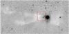 |
Fig. 1 Wide R-band view of the main concentration of dust in Lupus 3, from the images obtained by Comerón et al. (2009). The rectangle has dimensions of 7′3 × 7′4 and indicates the position of the field near the bright pair HR 5999/6000 investigated in this work. East is to the left and north to the top. |
The discovery of extremely low-mass objects in very young aggregates is complicated by the patchy extinction by foreground dust in the remnants of the parental molecular cloud, rapid evolution in the early phases, and possible distortions of the photospheric spectral energy distribution by accretion and circumstellar material emission. However, much progress has been made in the last decade with the discovery of ever fainter, less massive members now reaching down to a few Jupiter masses in some nearby star-forming regions (e.g. Luhman 2007; Luhman et al. 2009; Spezzi et al. 2008; Bihain et al. 2009; Boudreault & Bailer-Jones 2009; Scholz et al. 2009; Haisch et al. 2010; Geers et al. 2011; Lodieu et al. 2011, for some recent surveys). Much of the progress has come from dedicated surveys using wide-field instruments complemented by follow-up spectroscopy. However, reaching down to the very lowest masses of objects that may be formed out of molecular core contraction and fragmentation requires deep observations that currently fall within the domain of instrumentation at 8 m-class telescopes, even for the nearest star-forming regions.
The central parts of the Lupus 3 star-forming region (Comerón 2008) offer an interesting trade-off of factors in the search for extremely low-mass objects. Lupus 3 contains a very young aggregate that includes star formation activity going on even now (Tachihara et al. 2007) and is relatively nearby at ~200 pc from the Sun (see discussion on different distance determinations in Comerón 2008). Its relatively high galactic latitude (b ≃ 9°) implies a much lower density of background objects than in regions closer to the galactic plane, such as the Serpens clouds (Oliveira et al. 2009). The areal density of members near its center, dominated by the Herbig Ae/Be stars HR 5999 and HR 6000, is much higher than in other aggregates at a similar distance from the Sun, like Taurus and Chamaeleon I, and high densities of members are found even in regions of low extinction. Furthermore, hints of a mass function that is overabundant in very low-mass stars have been found in previous work (Hughes et al. 1994; López Martí et al. 2005). Given the large number of likely and confirmed members that can be found even in a relatively small field of view a few arcminutes across, deep imaging of the regions with the highest stellar densities thus appears a promising approach to searching for the faintest members of the aggregate.
This paper reports on a deep search for cool objects (Teff < 3000 K) carried out with the ESO Very Large Telescope (VLT) in a region located east of the HR 5999/HR 6000 pair. Its position has been chosen to encompass the greatest concentration of young stellar objects in the area, with over 20 confirmed or candidate members identified by previous studies. Photometric selection criteria are proposed based on imaging in the far red and near infrared, and the nature of the cool objects detected in this way is discussed. The results are examined in light of the statistical expectations derived from a standard form of the initial mass function in the field and in the aggregate. It is concluded that, although some objects with temperatures well below 3000 K are present in the imaged area, all of them are almost certainly unrelated, very low-mass stars in the field, and no Lupus 3 members with substellar mass are identified in this survey. It is also found that nearly half of the new young stellar objects in the field proposed by recent surveys are actually not confirmed as such and are most likely unrelated to the star-forming clouds. Although of limited significance owing to small number statistics, the results presented here argue against a high abundance of brown dwarfs in Lupus 3.
2. Observations
2.1. The target region
Star formation in Lupus 3 is concentrated in a dark cloud measuring approximately 0.7° × 0.3° elongated in the east-west direction, with the HR 5999/HR 6000 pair located roughly in its densest part. Using objective prism spectroscopy, a crowded group of T Tauri stars around the pair was first noticed by Thé (1962) and further expanded by Schwartz (1977). The vast majority of sources identified by Schwartz (1977) were confirmed as T Tauri stars by Hughes et al. (1994) using long-slit spectroscopy. Dedicated searches for fainter members in this region have been carried out by Nakajima et al. (2000) using near-infrared imaging, Comerón et al. (2003) using slitless spectroscopy, and López Martí et al. (2005) using narrow-band imaging through filters sensitive to Hα emission and temperature-sensitive continuum features. A highly complete census of young stellar objects with warm circumstellar dust has been provided by the Spitzer Legacy Program “From protostellar cores to planet-forming disks” (Evans et al. 2003; Merín et al. 2008). Several dense cores (Teixeira et al. 2005), the possible protostellar object Lupus 3 MMS (Tachihara et al. 2007), and several Herbig-Haro objects (Wang & Henning 2009) indicate that star formation has taken place in the region in the very recent past and will probably extend into the future.
The richest concentration of young stellar objects in the region is found due east of the HR 5999/HR 6000 pair, in the region that is the target of the survey presented here. An inventory of known sources in this area and a discussion of the actual membership of candidates is discussed below in Sect. 5.2, and Fig. 1 shows the area outlined against the larger scale structure of Lupus 3.
The southern and southeastern parts of the target field are partly covered by heavy dark nebulosity with associated dust column densities high enough to provide an opaque screen against background stars even in the KS band. While extinctions of up to AV ~ 20 mag have been reported by Nakajima et al. (2000) in this region, the colors of the reddest sources seen through the cloud in the deep images presented here indicate that the extinction reaches above AV ~ 50 in the most obscured areas. The protostellar source Lupus 3 MMS is embedded in this nebulosity. However, most of the imaged field has a much lower extinction, generally in the AV = 1−5 mag range.
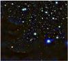 |
Fig. 2 Color composite of the 7′3 × 7′4 deep field observed with the VLT. Blue corresponds to the I band observed with FORS2, and green and red to the J and KS bands, respectively, observed with HAWK-I. The images used in this composite were obtained by stacking together the observations obtained through each filter on the different nights in which the observations were carried out. Heavy reddening is present only along the south and east edges of the field, covering approximately 30% of the area. The nebular object seen around mid height near the left edge of the field is the Herbig-Haro object HH 78, which has its origin at the embedded Class 0 source Lupus3 MMS (Tachihara et al. 2007). |
2.2. VLT observations
The observations presented in this paper were carried out using the FORS2 (far red) and HAWK-I (near infrared) imaging instruments at the VLT. Both instruments cover a similar field of view, 6′8 and 7′5 in side, respectively. The observations were carried out in service mode between April and July 2008. The precise coordinates of the center of the target region are α(2000) = 16h09m02s, δ(2000) = −39°04′49′′, and they were chosen so as to exclude bright stars in the field, which may produce heavy saturation or ghosts. It was, however, not possible to exclude stars bright enough in I to produce bleeding along detector rows, unless very short exposure times in that band were used, leading to prohibitively large detector readout overheads. The total area covered in all filters measures 7′4 × 7′3. An image of the field is shown in Fig. 2. Image processing was carried out using IRAF1-based scripts.
2.2.1. HAWK-I observations
The near-infrared broad-band observations were split into ten observing blocks (OBs), with a breakdown of four OBs in the J band (1.25 μm), four in the H band (1.65 μm), and two in the KS band (2.15 μm). Each OB in J consisted of 30 individual pointing positions of the telescope within a jitter box of 30′′ amplitude. On each position, two exposures of 50 s each were obtained and averaged on-detector. The respective numbers for the OBs in the H band are 60 pointing positions, nine exposures, and 10 s per exposure; and for the KS band, 30 pointing positions, nine exposures, and 10 s per exposure. The observations were affected by a problem of condensation in the entrance window of the instrument, solved only through an intervention that took place shortly after this program was completed. The problem had an almost negligible impact on the sensitivity of the observations, but it did produce a slowly rotating background pattern in the images. The rotation was slow enough for the pattern to effectively cancel out when subtracting two consecutive images from each other, but it prevented the use of the common “running sky” technique to subtract the background, in which a set (typically five or more) of images taken before and after the image to be background-subtracted, with telescope offsets in between, are median filtered and clipped. This would have involved the use of images taken over a time span in which the condensation pattern had rotated noticeably. For this reason, an alternative technique was employed by which only the combination of two images, taken immediately before and after the image to be background-subtracted, were used to construct the background. A crude removal of the stellar images in each of the two images to be used as background was performed by subtracting the other image from it, masking bright pixels with intensities more than 5σ above the standard deviation of the estimated background level, and then averaging the two masked images to form the background. The images in which the background had been subtracted in this way were then shifted to compensate for the telescope offsets, using the stellar positions as a reference to determine accurate shifts. Finally, the images shifted to a common reference frame were averaged, clipping off pixels deviating more than 5σ from the average. Given all of the telescope pointings in each OB the two-step clipping described above worked very well, even in the most crowded regions where the first clipping caused a large number of pixels to be masked. Flat field and dark frames obtained as part of the instrument calibration plan were used in the data reduction.
A first full set of near-infrared observations in the J, H and KS bands with HAWK-I was carried out on the night of 28/29 April 2008, in which half of the observing blocks in each band were executed, as listed in Table 1. The other half were executed on the night of 12/13 July 2008. In this way two complete sets of deep observations were obtained on or around two dates separated by over two months, thus giving the possibility of looking for variability. Finally, the observations in each filter obtained at all epochs were co-added into a single, deep image, with total exposure times of 3.3 h (J band), 3.0 h (H band), and 1.7 h (KS band).
As a complement to the broad-band observations, intermediate-band ones were also obtained through a methane filter centered on 1.575 μm and having a bandpass of 0.112 μm. This filter covers the approximate half of the H band not affected by the methane absorption feature that appears in the spectra of objects with temperatures below 1300 K. Very cool objects should thus stand out by appearing brighter in images taken using the methane filter than in the H band.
The methane filter observations were also composed of OBs each consisting of 35 telescope pointings and co-additions of four exposures of 20 s at each telescope pointing, thus totaling 0.78 h of exposure time per OB. The images were obtained over a period of three months as noted in Table 1, and the images produced by each individual OB were reduced with the same procedure as described for the broad-band images. All the methane-band images were then combined into a single deep one.
2.2.2. FORS2 observations
The I-band (0.768 μm) observations with FORS2 were carried out in five different epochs as noted in Table 1. Each observation was defined in an OB consisting of several exposures of 238 s each, with telescope offsets in between. Given the many pointings available within each OB, the processing of the I-band images was done using the same process as described above for the infrared images. Sky flat-field and bias frames obtained as part of the regular instrument calibration plan were used. Combined images for each night were produced, and then combined again to produce a single deep image with an equivalent exposure time of 5.75 h. The images resulting from each night of observation were also separately analyzed to enable the identification of variable objects.
2.2.3. Calibration
Log of observations.
The reduced images were registered and distortion-corrected with the IRAF GEOMAP and GEOTRANS tasks, using 2MASS Point Source Catalogue (Skrutskie et al. 2006) sources in the field of view for astrometric reference. Once placed on a common reference frame, the combined images in all filters were stacked to gain depth, and sources were automatically detected in them using DAOFIND (Stetson 1987). A master source list of 17 372 objects in the entire field of view was produced in this way.
Point spread function (PSF) photometry was carried out on the original images by automatically selecting a suitable set of PSF reference stars in each of them. To ensure that slightly saturated stars or stars with very close companions were excluded from the list of PSF reference stars, PSF photometry of the reference stars themselves was carried out and the χ2 statistics of the fit was used to identify stars with deviant PSF. To obtain the photometry of all the objects detected in the master source catalog, the PSF thus obtained was fitted to them using the ALLSTAR task in DAOPHOT (Stetson 1987). The fit was carried out by splitting the master source list into blocks of 100 sources, in descending order of brightness as estimated using approximate aperture photometry obtained with the PHOT task. The scaled PSFs fitted to each star in the block was subtracted from the image, and PSF photometry of the subsequent block of stars was then carried out with the images of the brighter stars largely removed, except in the cases of bright, saturated stars for which the subtraction of the fitted PSF left significant residuals. This greatly improved the accuracy of the fits for faint stars near brighter ones. Clearly extended sources, or sources for which a poor fit was obtained, were identified and excluded from further analysis in the relevant filter on the basis of the χ2 statistics and the source image parameters obtained from the fit.
Saturation and 5σ magnitude limits in the stacked images.
Photometric calibration was carried out by cross-matching the astrometric positions of the detected sources with the catalog of RCICzWFIJHKS photometry in Lupus of Comerón et al. (2009). The source of JHKS photometry in that work is the 2MASS Point Source Catalog, whereas IC photometry was obtained by Comerón et al. (2009) from the observation of standard star fields. The combination of the Bessell I filter used in the present observations and the detector throughput of FORS2 results in a response curve similar to that defining the IC band (Bessell 1990). The response curve of HAWK-I using the JHKS filters is very similar to that of the 2MASS photometric system. Therefore, no color terms were considered in any of the filters. The comparison between the instrumental magnitudes obtained here and the system magnitudes in Comerón et al. (2009) clearly shows the saturation level in each filter and field, as well as the limiting magnitudes, which are given in Table 2. For the sake of completeness in the catalog of point sources, the 2MASS JHKS magnitudes were used for bright stars above the saturation level in the J, H, and KS bands, whereas the IC magnitudes from Comerón et al. (2009) were used to replace the I magnitudes obtained for stars that appear saturated in that band in the present FORS2 observations. Finally, the instrumental zeropoint in the methane filter was derived by imposing the difference between the magnitude in that filter and the H magnitude to average to zero.
3. Selection criteria
The spectral energy distribution of stars and brown dwarfs at temperatures below ~3000 K makes their far red and near infrared colors markedly different from those of any other objects. The strength of molecular bands shortwards of 1 μm at temperatures between 2000 and 3000 K, the formation of dust in the atmosphere around 2000 K, and the onset of methane absorption near 1000 K produce very red I − J colors, while the JHKS colors become increasingly red as temperature decreases until the point where dust grains with sizes over ~1 μm sediment below the photosphere, marking the transition between the L and T spectral types (Kirkpatrick 1995) and the sudden bluing of the JHK colors.
Whereas current evolutionary models are able to reproduce the overall characteristics of the spectral energy distributions of very cool objects, significant differences exist between predicted and observed broad-band colors, particularly at visible wavelengths. Model uncertainties are expected to be greater in very young aggregates owing to the influence of the initial conditions (Baraffe et al. 2002), the large difference between the surface gravities of very young objects and of field objects at the same temperature, and other factors that may lead to significant mismatches between model predictions and observations at the youngest ages (Marley et al. 2007).
The identification of cool objects is made here not by relying on concrete model predictions of their colors, but rather by taking advantage of the spectral energy distribution of normal stars with temperatures above ~3000 K in the 0.7−2.3 μm region constraining the intrinsic colors to a relatively narrow range not accessible to cooler objects, regardless of the amount of extinction. The availability of photometry in four bands and the relationship among the values of extinction in each band, given by the interstellar extinction law, makes it possible to define two independent reddening-free indices, such as ![Mathematical equation: \begin{eqnarray} &[F]&\, = (I_{\rm C}-J) - 1.561 (J-K_{\rm S}) \\ &[G]&\, = (J-H) - 1.532 (H-K_{\rm S}), \arraycolsep1.75pt \end{eqnarray}](/articles/aa/full_html/2011/07/aa16523-11/aa16523-11-eq53.png) where the numerical coefficients on the right hand side are derived from the interstellar extinction law of Cardelli et al. (1989) using a total-to-selective extinction ratio RV = 5.5, which is more appropriate for dense clouds than the canonical RV = 3.1 of the general interstellar medium. The value RV = 3.1 may actually be more adequate for distant background sources seen through areas of low extinction of the cloud, because the extinction in their direction is probably dominated by smaller dust grains in the diffuse interstellar gas. However, the coefficients vary by less than 3% when either RV value is used, which makes the indices [F] and [G] defined above virtually reddening-free for any reasonable changes in the extinction law along the line of sight.
where the numerical coefficients on the right hand side are derived from the interstellar extinction law of Cardelli et al. (1989) using a total-to-selective extinction ratio RV = 5.5, which is more appropriate for dense clouds than the canonical RV = 3.1 of the general interstellar medium. The value RV = 3.1 may actually be more adequate for distant background sources seen through areas of low extinction of the cloud, because the extinction in their direction is probably dominated by smaller dust grains in the diffuse interstellar gas. However, the coefficients vary by less than 3% when either RV value is used, which makes the indices [F] and [G] defined above virtually reddening-free for any reasonable changes in the extinction law along the line of sight.
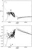 |
Fig. 3 Expected behavior of the [F] and [G] reddening-free indices defined in Sect. 3 as a function of the stellar and substellar effective temperature. The solid line corresponds to the models of Chabrier et al. (2000) that include dust formation in the atmosphere, whereas the dotted line reproduces the models of Baraffe et al. (2003) in which dust species can sediment below the photosphere. The latter should represent the behavior of objects with Teff < 1400 K. The actual indices of cool objects with spectral classifications are plotted. Filled circles are confirmed members of the Chamaeleon I star-forming region from Luhman (2007), with magnitudes from that work except for members identified previous to Luhman’s study, for which the magnitudes are from Lawson et al. (1996). Also plotted are field cool dwarfs from Leggett et al. (2000) (open triangles), Dahn et al. (2002) (open circles), and Liebert & Gizis (2006) (open squares). For higher temperatures, the average colors of stars with solar metallicity (filled squares) and [Fe/H] = −2.5 (filled triangles) from Alonso et al. (1996) are given. Stars hotter than Teff > 3000 K have their [F] and [G] indices confined to a narrow permitted range well separated from the values reached by cooler objects. |
ICJHKS photometry of cool objects in the field in the co-added images.
Figure 3 shows the behavior of [F] and [G] with temperature as predicted by the evolutionary models of Chabrier et al. (2000) and Baraffe et al. (2003) for an age of 5 Myr, extended for masses above 0.1 M⊙ with the models of Baraffe et al. (1998) at the same age, and with the colors of main sequence stars from Kenyon & Hartmann (1995) for temperatures above 4000 K. The variations predicted by models among objects of different masses and ages having the same effective temperature are small, and the plots in Fig. 3 depend little on the assumed age. Figure 3 also shows the actual indices of several samples of spectroscopically classified cool objects, both in the field and in a star forming region. Temperatures for the young members of the Chamaeleon I region are from Luhman (2007). For field objects, a linear dependence between spectral subtype and temperature that provides a good fit to the temperatures derived by Dahn et al. (2002) down to L8 (Teff = 1400 K) has been used. A similar linear dependence approximates the temperature-spectral type relationship derived from Golimowski et al. (2004) data for types later than T5. A constant temperature Teff = 1400 K has been assumed for objects with spectral types between L8 and T5; see also Kirkpatrick (1995) for a discussion on the temperature-spectral type relationship for cool dwarfs. In all cases, cool stars with temperatures below ~3000 K are characterized by nearly zero or negative values of [G] that are inaccessible to warmer photospheres, as well as by high positive values of [F] for Teff > 1700 K that are also unique. As the JHKS colors become intrinsically redder due to the formation of large dust grains, a narrow temperature interval is predicted by models around 1500 < Teff (K) < 1700 in which the [F] index covers the same values as those of normal stars, while [G] remains negative, although this rapid decline in [F] is not seen among the actual objects plotted in Fig. 3. Finally, at the coolest temperatures both [F] and [G] can attain extreme values, their behavior depending on the details of the grain sedimentation process below the photosphere. The dust sedimentation models of Baraffe et al. (2003) qualitatively reproduce this feature.
Candidate cool objects have thus been selected as those having either [F] > 0.6 or [F] < −0.5, or those having either [G] < 0.0 or [G] > 0.6, even after accounting for the estimated measurement uncertainties. This criterion may thus include objects undetected in the IC or J bands, for which only lower limits in [F] and [G] can be obtained. Such criteria are only intended to exclude those stars from the selection whose colors are consistent with reddened photospheres with Teff > 3000 K, which turn out to compose the vast majority of sources in the sample. It is thus not based on any actual fit to the spectral energy distributions of cool objects.
The observations presented here should be able to detect unreddened objects with effective temperatures that are cool enough to result in the condensation of large dust grains below the photosphere. At such temperatures molecular absorption by methane and H2 strongly reduces the emitted flux in the KS band. Given the depth in the different bands of the observations presented here, the detection limit for color-based recognition of such cool objects when lightly reddened is set in practice by the KS band flux. At the KS = 21.3 3σ detection limit, the corresponding absolute magnitude MKS = 14.8 is predicted by the evolutionary models of Baraffe et al. (2003) for objects of Teff < 900 K, virtually regardless of the age. The corresponding mass does depend on the age though, and it ranges from < 1 MJup for 1 Myr to 1.5 MJup for 5 Myr. These observations thus span a sizeable part of the range where methane absorption produces a prominent decrease of flux in the red part of the H band, making possible the independent detection of objects with Teff < 1300 K through the negative value of the [CH4] − H color.
4. Results
As expected, the vast majority of objects in the observed Lupus 3 field have [F] , [G] indices consistent with temperatures above Teff > 3000 K. Upon close inspection, most objects outside that range happen to be very close to brighter sources or to lie in the proximities of saturating stars, thus making the photometric measurements unreliable. A few others turn out to be marginally resolved faint galaxies as revealed by the residuals of their PSF fits. However, after close inspection of each candidate, a total of 17 relatively isolated point sources, listed in Table 3, are identified as sound candidate cool objects. Objects in Table 3 are named after their J2000 coordinates, and their photometry is performed on the images obtained by co-adding all the epochs in which observations through a given filter were obtained.
All sources in Table 3 are characterized by positive values of [F] and values of [G] that are either negative or very close to zero, in consistency with the behavior described above for cool objects with 1700 < Teff(K) < 3000. As noted above, the selection criteria require either of those indices to be outside the range covered by normal photospheres. That for all candidates selected both indices lie in the range expected for cool objects thus supports their character. All objects found to be outside the [F] range covered by hotter photospheres are faint but still detected at IC, thanks to the depth of the observations in that band, and their [F] values (as opposed to only lower limits) can thus be computed. No objects with the extreme values of [F] and [G] that would be expected from very cool photospheres depleted in small dust grains (Teff < 1000 K) are identified in the observed region, despite the deep detection limits discussed in Sect. 3.
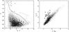 |
Fig. 4 Location of the cool stars identified in the observed Lupus 3 field (filled dots) in the (IC − J,J) and (J − KS),(IC − J) diagrams. The location of such cool objects above the main band defined by the photospheres of hotter stars reddened by various amounts in the right hand diagram is clear. Their position in the (IC − J,J) lies in all cases well below the 5 Myr isochrone from Chabrier et al. (2000), indicating that these objects are not members of the Lupus 3 star-forming region. For comparison, the location of known members of Lupus 3 (Sect. 5.2) is marked with empty circles in the color–magnitude diagram on the left. The dotted line in the (IC − J,J) diagram indicates an extinction vector corresponding to AV = 5 mag. |
The location of these objects in color–magnitude diagrams indicates that all of them are too faint to be members of the Lupus 3 region, as seen in the left panel of Fig. 4, where they lie far below the 5 Myr isochrone of Chabrier et al. (2000). Most of the known members of Lupus 3 in the same field (Sect. 5.2) lie above it, indicating younger ages and implying that the 5 Myr isochrone may be taken as the lower boundary of the region of the color–magnitude diagram accessible to young members of Lupus 3. Despite the uncertainties in evolutionary tracks and the non overlapping range of colors between the known members and the candidate cool objects, the conclusion that the new cool objects identified are actually evolved field sources appearing in the direction of Lupus 3, rather than young members of it, seems firmly established. No evidence of new members of Lupus 3 with temperatures below Teff ~ 3000 K, hence with masses below the substellar limit, is thus found in the observations presented here. The colors of the 17 objects in Table 3 all indicate of late-M or early-L spectral type photospheres with some amount of foreground reddening. The large scatter in intrinsic colors at very low temperatures, reflected in the scatter in [F] and [G] values at a given temperature in Fig. 3, prevents any accurate determination of the temperature and any estimate of the main-sequence mass, but the [F] , [G] limits chosen for the selection of cool objects guarantees Teff < 2800 K for all the objects listed in Table 3.
The absence of objects with very low temperatures in the Lupus 3 field is independently confirmed by the absence of any source with clearly negative [CH4] − H color, which would be distinctive of objects with Teff < 1300 K having a mid-T or later spectral type.
5. Discussion
5.1. Field population
As shown by Caballero et al. (2008), the field population of very cool stars at faint magnitudes can easily dominate the members of the same temperature in young aggregates. The estimate of the expected number of cool field objects in the images presented here is made somewhat difficult by the irregular extinction across the Lupus 3 field, which in turn makes the distance up to which objects would be detected dependent on the direction. Fortunately, as is apparent from Fig. 2, the imaged field can be roughly split into a “high extinction” region, corresponding to ~30% in area, where dense clouds render the vast majority of sources located behind undetectable at the shortest wavelengths, and the remaining ~70% of the area where the extinction is much lower, and where all the detected cool sources are located.
To estimate the number of objects at temperatures Teff < 2800 K that may be statistically expected in the low extinction portion of the Lupus 3 field, the present-day mass function in the local galactic disk in the form given by Chabrier (2005) has then been used to estimate the number of cool stars up to an unreddened magnitude Jlim = 20.7 ± 0.5, which is taken as a representative limit given the magnitudes of the objects listed in Table 3 and the typical value of the extinction, AJ ≃ 1 mag, as inferred from the color–color magnitude diagrams of the area, which are dominated by background sources. The quoted uncertainty in J accounts for a combination of the scatter in extinction and the faintest J magnitude for which a very red (I − J) color can be unambiguously identified given the JHKS colors, which is a function of the reddening of the object and of its intrinsic colors. Given the low galactic latitude (b = + 9°) of the Lupus 3 field and the relatively nearby horizon up to which such cool stars can be detected in these observations, departures in number density of stars from the local value due to the scale height or the radial scale length of the galactic disk can be neglected (a thorough general treatment of these effects can be found in Caballero et al. 2008). The expected numbers of very low-mass stars with temperatures Teff < 2800 K obtained in this way are  across the approximately 0.011 square arcminutes of lightly obscured area of the field, in good agreement with the number of cool stars actually found.
5.2. Known cloud members
Confirmed and excluded candidate young stellar objects in the target region.
Despite its limited extent (0.42 pc × 0.43 pc projected area at the distance of 200 pc) with respect to the overall size of the complex, the imaged field contains a high concentration of young stellar objects in Lupus 3. At least nine of the objects previously identified as young stellar objects can be reliably considered as members of the star forming region, and eight of those have published spectroscopic classifications and estimates of their mass. Most of the others have been previously classified as candidate members on the basis of their broad-band near- and mid-infrared photometry. For the latter, the bases on which the initial classification as candidates was produced can be reexamined now thanks to the higher angular resolution of the observations presented here, as well as to the improved photometry. In this way several previous candidates are excluded as possible members. The final census considered here is listed in Table 4, together with an estimate of the mass when available. Excluded candidates are also listed there, indicating the reasons for exclusion. From the list of 15 candidates considered to be true members of the star-forming region, ten are projected on the low extinction area, with the remaining five being significantly embedded in nebulosity of high column density.
Several binary stars among the members of Lupus 3 have been identified by Reipurth & Zinnecker (1993), none of which is in the field covered by the new observations. However, a detailed visual inspection of the images of the know members shows that Par-Lup3-3 is actually a close pair with two components of similar brightness separated by ≃ 0′′3 in the north-south direction.
A faint close companion is also detected in the KS-band images of the jet-driving, very low-mass star Par-Lup3-4 (Fernández & Comerón 2005; Huélamo et al. 2010; Comerón & Fernández 2011). The companion is located 1′′2 to the east-northeast of the central star, at a position angle roughly perpendicular to that of the jet axis. The proximity to Par-Lup3-4 and the brightness difference between both objects makes determining the magnitude of the companion very difficult, with a best estimate of KS = 20.4 ± 0.5. The object is not visible at shorter wavelengths. Assuming an age of 1 Myr, which seems plausible and even conservative given the signs of extreme youth of Par-Lup3-4, this magnitude implies a mass of only ~1−2 MJup. The crowding on the field leaves open the possibility that the apparent companion may actually be an unrelated background star, but the peculiar character of Par-Lup3-4 makes further observations aiming at confirming of the possible binarity of Par-Lup3-4 interesting. No other likely binary companions are identified for the other stars in Table 4.
5.3. Expected new members and the mass function
Although the accuracy of the mass estimates varies widely among the members of the cloud, the 15 young stellar objects listed in Table 4 clearly probe the Lupus 3 population down to a spectral type of about M6.5. The temperature corresponding to this spectral type is Teff ≃ 3000 K (Luhman et al. 2003), and the mass is near the substellar limit, M = 0.075 M⊙, almost independently of the age within the range found in star-forming regions due to the early evolution at nearly constant Teff for objects around this mass (Chabrier et al. 2000). Of those, ten are projected on low extinction (AV < 5 mag) areas where the present observations are sensitive to the extremely low masses discussed at the end of Sect. 3. Taking these ten members as a complete sampling of the stellar mass function down to the hydrogen-burning limit, the stars-to-brown dwarfs ratio derived from other star-forming regions should provide a direct estimate of the number of brown dwarf members expected in the observed area. The ratio has been found to be around 4–5 in regions such as Chamaeleon I (Luhman 2007, recently confirmed by Mužić 2011), ρ Ophiuchi (Geers et al. 2011), IC 348 (Luhman et al. 2003), or the Orion Nebula Cluster (Slesnick et al. 2004); see also Andersen et al. (2008). Based on this, the expected number of brown dwarf members in the observed Lupus 3 field is N ≃ 2 − 3. A somewhat lower ratio has been inferred for the outskirts of Chamaeleon I (Luhman 2007) and Taurus (Luhman et al. 2009), which if applied to Lupus 3 would reduce the expectation to 1–2 new members. Given the small number statistics, this expectation can be considered to be consistent with the finding that none of the cool objects identified in these observations is a member of the star-forming cloud. It does not necessarily imply a sharper drop in the mass function in Lupus or an anomalous lack of brown dwarfs, a possibility that could only be investigated through surveys of larger areas.
It may be noted that the tail in the distribution of late spectral types found by Hughes et al. (1994) in Lupus, as compared to other nearby star-forming regions and supported by further surveys (López Martí et al. 2005), could have hinted at an unusually low star-to-brown dwarf ratio that the present study should have been able to confirm. Indications of such a low ratio have been presented for NGC 1333 by Wilking et al. (2004) and Greissl et al. (2007), and supported by Scholz et al. (2009) using near-infrared spectroscopic classifications of new candidate members. The ratio derived in this way should be taken with caution given that the dividing line between stars and brown dwarfs lies near the peak of the mass function, thus making such a ratio particularly sensitive to systematic effects that may tend to move the estimated masses of low-mass members to either side of the boundary (Luhman 2007). The comparison between results based on visible and near-infrared spectroscopy may be affected by such biases, given the greater uncertainties in near-infrared spectral classifications. However, Lodieu et al. (2011) have recently used visible spectroscopy to derive a star-to-brown dwarf ratio of only 2.5 for the Upper Scorpius association, adjacent to the Lupus clouds, based on spectroscopy in the visible. The departure with respect to values found in other regions is mainly due to an overabundance of brown dwarfs with masses below ~ 0.04 M⊙ that includes a possible secondary peak of the mass function around 0.015 M⊙. Such a mass distribution in the Lupus 3 field would lead to the expectation of 4 ± 2 new cool brown dwarfs, which is somewhat harder to reconcile with the lack of new members found in the present study. An upturn in the mass function near the deuterium-burning limit has also been suggested by Muench et al. (2002) for the Trapezium cluster, but it was not confirmed by observations of a larger area by Robberto et al. (2010), although the existence of objects near or below the deuterium-burning limit is required to reproduce the overall shape of the luminosity function in that cluster (Weights et al. 2009).
The existence of even lower mass objects in star-forming regions and young aggregates appears to be well established, as is best illustrated by the numerous recent studies of the σ Orionis aggregate (e.g. Zapatero Osorio et al. 2002, 2008; Caballero et al. 2008; Lodieu et al. 2009; Bihain et al. 2009) and other regions (Weights et al. 2009; Marsh et al. 2010), where objects with T-dwarf-like spectra have been found. Despite the availability of deep H- and CH4-band imaging, no candidate T-like object is identified in the present study. The abundances of such objects in young aggregates are still controversial, and it cannot be ruled out that large variations in the populations exist among different regions. Bihain et al. (2009) argue that such objects, although present, are exceedingly rare in the σ Orionis aggregate, and Scholz et al. (2009) find that planetary-mass objects are altogether absent from NGC 1333, despite an apparent overabundance of higher mass brown dwarfs as noted above. On the other end, Haisch et al. (2010) report the identification of 22 candidate sources with evidence of methane absorption in their spectral energy distribution in an area of only 0.26 sq. degrees in the ρ Ophiuchi embedded cluster. While the implications for the general shape of the mass function are not clear from the results presented in that paper, and spectroscopic confirmation of the candidates is still needed, it appears at least qualitatively that such results, if confirmed, would argue against freely floating objects, with 1–2 MJup, being extremely rare. Still, even if their abundance were as high as suggested by the results of Haisch (2010), the area imaged in the present study would have made the finding of any objects rather serendipitous, and the fact that none is detected bears little if any significance on the statistics of such objects in Lupus 3.
6. Conclusions
This paper presents deep ICJHKS imaging with the VLT of a densely populated region of the Lupus 3 star-forming region. Its depth leads to detection limits well into the giant-planet-mass regime, probing down to sub-Jupiter masses if the age is below ~2 Myr and to ≃1.5 MJup for an age of 5 Myr. Although the detection limits are considerably fainter than those reached by other contemporary surveys of star-forming regions and young stellar aggregates at similar distances, its areal coverage is much smaller. However, this is partly compensated for by the large number of confirmed and candidate young stellar objects that have been identified in the field by previous studies, which leads to the a priori expectation of identifying a few new brown dwarfs. The survey also includes deep imaging through a “CH4” filter covering the H-band continuum to the blue of the broad methane absorption feature that characterizes the spectral energy distribution of T dwarfs, so that any possible objects with temperatures below Teff ≃ 1300 K can be identified through comparing of the H and CH4 magnitudes. The conclusions of this work can be summarized as follows.
-
A few candidate faint cool objects are identified by means of a combination of two reddening-free indices defined on the basis of the ICJHKS colors. The values of these indices are constrained to a narrow range in the case of normal stellar photospheres warmer than 3000 K. After careful examination of each of them, a final list of 17 objects with temperatures below 2800 K is obtained. All of them are characterized by very red IC − J colors that cannot be accounted for solely by extinction, given their spectral energy distribution at longer wavelengths.
-
All 17 objects detected in this way are significantly fainter than expected for actual members of the Lupus clouds, and are most likely background, evolved very low-mass stars rather than brown dwarf members of Lupus 3. Their number agrees with the statistical expectation of a background population down to the sensitivity limit of the observations presented here.
-
A reexamination of the known confirmed and candidate young stellar objects reported by previous studies leads to the conclusion that eight of them are not true members of Lupus 3 and should thus be excluded from the census. Two others are X-ray sources without any optical counterpart so are also discarded as likely background active galactic nuclei. The census of confirmed and likely young stellar objects in the surveyed area is thus reduced to 15. Of these, five are deeply embedded in the most obscured parts of the clouds.
-
Par-Lup3-3, a confirmed M4.5 member of the star-forming region, is found to be a close pair formed by members of similar brightness separated by ≃ 0′′3. Also Par-Lup3-4, an M5 object with prominent accretion and mass-loss signatures that drives a short jet, may be a binary, as suggested by a possible companion of KS ~ 20.4 at 1′′2 from the primary. If physically related to Par-Lup3-4, the companion would have an estimated mass of 1 − 2 MJup.
-
The non detection of any new substellar objects is somewhat surprising in view of the number of confirmed stellar members in the same observed area, which lead to an expectation of approximately two or three new brown dwarfs based on the stars-to-brown dwarfs ratios derived for other star-forming regions. Although of limited statistical significance given the small numbers involved, a mass function rich in substellar objects that may have been suggested by the previously reported abundance of mid M-type stars in Lupus 3 is not supported by these new observations. The lack of brown dwarfs in the surveyed area includes objects with indications of methane absorption in their spectral energy distribution.
The results found in this work concerning the detection of new brown dwarfs in Lupus 3 indicate that wider area surveys will be needed to characterize the bottom of the mass function in this region, whose potential for such studies continue to be extremely interesting. Despite its relative richness, the area targeted in this work only contains a minor fraction of the total confirmed population of stellar members of the star-forming region, which is in itself sufficiently abundant to provide a robust determination of the complete mass function and, perhaps, of the mass below which no isolated objects can form, if surveyed to an adequate extent with a depth comparable to that of the present work.
IRAF is distributed by NOAO, which is operated by the Association of Universities for Research in Astronomy, Inc., under contract to the National Science Foundation.
Acknowledgments
I am thankful to the Paranal Science Operations staff for executing of the observations reported in this paper, and to Dr. Monika Petr-Gotzens and Dr. Bodo Ziegler at the ESO User Support Department, within the Data Management and Operations Division, for their support with the Phase 2 preparation of these observations. Dr. Petr-Gotzens’ careful follow-up on the quality of the HAWK-I data is especially appreciated. I also express my gratitude to the staff of the Specola Vaticana, where most of the analysis presented in this paper was carried out, for their warm hospitality. The careful refereeing of this paper by Dr. Kevin Luhman led to substantial improvements.
References
- Allen, P. R., Luhman, K. L., Myers, P. C., et al. 2007, ApJ, 655, 1095 [NASA ADS] [CrossRef] [Google Scholar]
- Alonso, A., Arribas, S., & Martínez-Roger, C. 1996, A&A, 313, 873 [NASA ADS] [Google Scholar]
- Andersen, M., Meyer, M. R., Greissl, J., & Aversa, A. 2008, ApJ, 683, L183 [NASA ADS] [CrossRef] [Google Scholar]
- Baraffe, I., Chabrier, G., Allard, F., & Hauschildt, P. H. 1998, A&A, 337, 403 [NASA ADS] [Google Scholar]
- Baraffe, I., Chabrier, G., Allard, F., & Hauschildt, P. H. 2002, A&A, 382, 563 [NASA ADS] [CrossRef] [EDP Sciences] [Google Scholar]
- Baraffe, I., Chabrier, G., Barman, T. S., Allard, F., & Hauschildt, P. H. 2003, A&A, 402, 701 [NASA ADS] [CrossRef] [EDP Sciences] [Google Scholar]
- Baraffe, I., Chabrier, G., & Gallardo, J. 2009, ApJ, 702, L27 [NASA ADS] [CrossRef] [Google Scholar]
- Bessell, M. 1990, PASP, 102, 1181 [NASA ADS] [CrossRef] [Google Scholar]
- Bihain, G., Rebolo, R., Zapatero Osorio, M. R., et al. 2009, A&A, 506, 1169 [NASA ADS] [CrossRef] [EDP Sciences] [Google Scholar]
- Boudreault, S., & Bailer-Jones, C. A. L. 2009, ApJ, 706, 1484 [NASA ADS] [CrossRef] [Google Scholar]
- Burrows, A., Hubbard, W. B., Lunine, J. I., & Liebert, J. 2001, Rev. Mod. Phys., 73, 719 [Google Scholar]
- Caballero, J. A., Béjar, V. J. S., Rebolo, R., et al. 2007, A&A, 470, 903 [NASA ADS] [CrossRef] [EDP Sciences] [Google Scholar]
- Caballero, J. A., Burgasser, A. J., & Klement, R. 2008, A&A, 488, 181 [NASA ADS] [CrossRef] [EDP Sciences] [Google Scholar]
- Cardelli, J. A., Clayton, G. C., & Mathis, J. S. 1989, ApJ, 345, 245 [NASA ADS] [CrossRef] [Google Scholar]
- Chabrier, G. 2003, PASP, 115, 763 [NASA ADS] [CrossRef] [Google Scholar]
- Chabrier, G. 2005, in The initial mass function 50 years later, ed. E. Corbelli et al. (Springer) [Google Scholar]
- Chabrier, G., & Baraffe, I. 2000, ARA&A, 38, 337 [NASA ADS] [CrossRef] [Google Scholar]
- Chabrier, G., Baraffe, I., Allard, F., & Hauschildt, P. 2000, ApJ, 542, 464 [NASA ADS] [CrossRef] [Google Scholar]
- Cieza, L., Padgett, F. L., Stapelfeldt, K. R., et al. 2007, ApJ, 667, 308 [NASA ADS] [CrossRef] [Google Scholar]
- Comerón, F. 2008, The Lupus clouds, in Handbook of Star Forming regions, ed. B. Reipurth, ASP Mon., 2 [Google Scholar]
- Comerón, F., & Fernández, M. 2011, A&A, 528, 99 [Google Scholar]
- Comerón, F., Fernández, M., Baraffe, I., Neuhäuser, R., & Kaas, A. A. 2003, A&A, 406, 1001 [NASA ADS] [CrossRef] [EDP Sciences] [Google Scholar]
- Comerón, F., Spezzi, L., & López Martí, B. 2009, A&A, 500, 1045 [NASA ADS] [CrossRef] [EDP Sciences] [Google Scholar]
- Dahn, C. C., Harris, H. C., Vrba, F. J., et al. 2002, AJ, 124, 1170 [NASA ADS] [CrossRef] [Google Scholar]
- Elmegreen, B. G. 2009, in The evolving ISM in the Milky Way and nearby galaxies, ed. K. Sheth, A. Noriega-Crespo, J. Ingalls, & R. Paladini, ssc.spitzer.caltech.edu/mtgs/ismevol/ [Google Scholar]
- Evans, N. J., Allen, L. E., Blake, G. A., et al. 2003, PASP, 115, 965 [NASA ADS] [CrossRef] [Google Scholar]
- Fernández, M., & Comerón, F. 2005, A&A, 440, 1119 [NASA ADS] [CrossRef] [EDP Sciences] [Google Scholar]
- Geers, V., Scholz, A., Jayawardhana, R., et al. 2011, ApJ, 726, 23 [NASA ADS] [CrossRef] [Google Scholar]
- Golimowski, D. A., Leggett, S. K., Marley, M. S., et al. 2004, AJ, 127, 3516 [NASA ADS] [CrossRef] [Google Scholar]
- Gondoin, P. 2006, A&A, 454, 595 [NASA ADS] [CrossRef] [EDP Sciences] [Google Scholar]
- Greissl, J., Meyer, M. R., Wilking, B. A., et al. 2007, AJ, 133, 1321 [NASA ADS] [CrossRef] [Google Scholar]
- Haisch, K. E., Barsony, M., & Tinney, C. 2010, ApJ, 719, L90 [NASA ADS] [CrossRef] [Google Scholar]
- Huélamo, N., Bouy, H., Pinte, C., et al. 2010, A&A, 523, 42 [Google Scholar]
- Hughes, J. H., Hartigan, P., Krautter, J., & Kelemen, J. 1994, AJ, 108, 1071 [NASA ADS] [CrossRef] [Google Scholar]
- Kenyon, S. J., & Hartmann, L. 1995, ApJS, 101, 117 [NASA ADS] [CrossRef] [Google Scholar]
- Kirkpatrick, J. D. 2005, ARA&A, 43, 195 [NASA ADS] [CrossRef] [Google Scholar]
- Krautter, J., Wichmann, R., Schmitt, J. H. M. M., et al. 1997, A&AS, 123, 329 [NASA ADS] [CrossRef] [EDP Sciences] [Google Scholar]
- Lawson, W. A., Feigelson, E. D., & Huenemorder, D. P. 1996, MNRAS, 280, 1071 [NASA ADS] [Google Scholar]
- Leggett, S. K., Allard, F., Dahn, C., et al. 2000, ApJ, 535, 965 [NASA ADS] [CrossRef] [Google Scholar]
- Liebert, J., & Gizis, J. E. 2006, PASP, 118, 659 [NASA ADS] [CrossRef] [Google Scholar]
- Lodieu, N., Zapatero Osorio, M. R., Rebolo, R., Martín, E. L., & Hambly, N. C. 2009, A&A, 505, 1115 [NASA ADS] [CrossRef] [EDP Sciences] [Google Scholar]
- Lodieu, N., Dobbie, P. D., & Hambly, N. C. 2011, A&A, 527, A24 [NASA ADS] [CrossRef] [EDP Sciences] [Google Scholar]
- López Martí, B., Eislöffel, J., & Mundt, R. 2005, A&A, 440, 139 [NASA ADS] [CrossRef] [EDP Sciences] [Google Scholar]
- Luhman, K. L. 2007, ApJS, 173, 104 [NASA ADS] [CrossRef] [Google Scholar]
- Luhman, K. L., Stauffer, J. R., Muench, A. A., et al. 2003, ApJ, 593, 1093 [NASA ADS] [CrossRef] [Google Scholar]
- Luhman, K. L., Mamajek, E. E., Allen, P. R., & Cruz, K. L. 2009, ApJ, 703, 399 [NASA ADS] [CrossRef] [Google Scholar]
- Marley, M. S., Fortney, J. J., Hubickyj, O., Bodenheimer, P., & Lissauer, J. J. 2007, ApJ, 655, 541 [NASA ADS] [CrossRef] [Google Scholar]
- Marsh, K. A., Plavchan, P., Kirkpatrick, J. D., et al. 2010, ApJ, 719, 550 [NASA ADS] [CrossRef] [Google Scholar]
- Merín, B., Jørgensen, J., Spezzi, L., et al. 2008, ApJS, 177, 551 [NASA ADS] [CrossRef] [Google Scholar]
- Muench, A. A., Lada, E. A., Lada, C. J., & Alves, J. 2002, ApJ, 573, 366 [NASA ADS] [CrossRef] [Google Scholar]
- Mužić, K., Scholz, A., Geers, V., Fissel, L., & Jayawardhana, R. 2011, ApJ, 732, 86 [NASA ADS] [CrossRef] [Google Scholar]
- Nakajima, Y., Tamura, M., Oasa, Y., & Nakajima, T. 2000, AJ, 119, 873 [NASA ADS] [CrossRef] [Google Scholar]
- Oliveira, I., Merín, B., Pontoppidan, K. M., et al. 2009, ApJ, 691, 672 [NASA ADS] [CrossRef] [Google Scholar]
- Quanz, S. P., Goldman, B., Henning, T., et al. 2010, ApJ, 708, 770 [NASA ADS] [CrossRef] [Google Scholar]
- Reipurth, B., & Clarke, C. 2001, AJ, 122, 432 [NASA ADS] [CrossRef] [Google Scholar]
- Reipurth, B., & Zinnecker, H. 1993, A&A, 278, 81 [NASA ADS] [Google Scholar]
- Robberto, M., Soderblom, D. R., Scandariato, G., et al. 2010, AJ, 139, 950 [NASA ADS] [CrossRef] [Google Scholar]
- Scholz, A., & Eislöffel, J. 2004, A&A, 421, 259 [NASA ADS] [CrossRef] [EDP Sciences] [Google Scholar]
- Scholz, A., Geers, V., Jayawardhana, R., et al. 2009, ApJ, 702, 805 [NASA ADS] [CrossRef] [Google Scholar]
- Schwartz, R. D. 1977, ApJS, 35, 161 [Google Scholar]
- Skrutskie Cutri, R. M., Stiening, R., et al. 2006, AJ, 131, 1163 [NASA ADS] [CrossRef] [Google Scholar]
- Slesnick, C. L., Hillenbrand, L. A., & Carpenter, J. M. 2004, ApJ, 610, 1045 [NASA ADS] [CrossRef] [Google Scholar]
- Spezzi, L., Alcalá, J. M., Covino, E., et al. 2008, ApJ, 680, 1295 [NASA ADS] [CrossRef] [Google Scholar]
- Stetson, P. B. 1987, PASP, 99, 191 [NASA ADS] [CrossRef] [Google Scholar]
- Tachihara, K., Rengel, M., Nakajima, Y., et al. 2007, ApJ, 659, 1382 [NASA ADS] [CrossRef] [Google Scholar]
- Teixeira, P. S., Lada, C. J., & Alves, J. F. 2005, ApJ, 629, 276 [CrossRef] [Google Scholar]
- Thé, P. S. 1962, Contrib. Bosscha Obs., 15 [Google Scholar]
- Wang, H., & Henning, Th. 2009, AJ, 138, 1072 [NASA ADS] [CrossRef] [Google Scholar]
- Weights, D. J., Lucas, P. W., Roche, P. F., Pinfield, D. J., & Riddick, F. 2009, MNRAS, 392, 817 [NASA ADS] [CrossRef] [Google Scholar]
- Wilking, B. A., Meyer, M. R., Greene, T. P., Mikhail, A., & Carlson, G. 2004, AJ, 127, 1131 [NASA ADS] [CrossRef] [Google Scholar]
- Zapatero Osorio, M. R., Béjar, V. J. S., Martín, E. L., et al. 2002, ApJ, 578, 536 [NASA ADS] [CrossRef] [Google Scholar]
- Zapatero Osorio, M. R., Béjar, V. J. S., Bihain, G., et al. 2008, A&A, 477, 895 [NASA ADS] [CrossRef] [EDP Sciences] [Google Scholar]
All Tables
All Figures
|
Fig. 1 Wide R-band view of the main concentration of dust in Lupus 3, from the images obtained by Comerón et al. (2009). The rectangle has dimensions of 7′3 × 7′4 and indicates the position of the field near the bright pair HR 5999/6000 investigated in this work. East is to the left and north to the top. |
| In the text | |
|
Fig. 2 Color composite of the 7′3 × 7′4 deep field observed with the VLT. Blue corresponds to the I band observed with FORS2, and green and red to the J and KS bands, respectively, observed with HAWK-I. The images used in this composite were obtained by stacking together the observations obtained through each filter on the different nights in which the observations were carried out. Heavy reddening is present only along the south and east edges of the field, covering approximately 30% of the area. The nebular object seen around mid height near the left edge of the field is the Herbig-Haro object HH 78, which has its origin at the embedded Class 0 source Lupus3 MMS (Tachihara et al. 2007). |
| In the text | |
|
Fig. 3 Expected behavior of the [F] and [G] reddening-free indices defined in Sect. 3 as a function of the stellar and substellar effective temperature. The solid line corresponds to the models of Chabrier et al. (2000) that include dust formation in the atmosphere, whereas the dotted line reproduces the models of Baraffe et al. (2003) in which dust species can sediment below the photosphere. The latter should represent the behavior of objects with Teff < 1400 K. The actual indices of cool objects with spectral classifications are plotted. Filled circles are confirmed members of the Chamaeleon I star-forming region from Luhman (2007), with magnitudes from that work except for members identified previous to Luhman’s study, for which the magnitudes are from Lawson et al. (1996). Also plotted are field cool dwarfs from Leggett et al. (2000) (open triangles), Dahn et al. (2002) (open circles), and Liebert & Gizis (2006) (open squares). For higher temperatures, the average colors of stars with solar metallicity (filled squares) and [Fe/H] = −2.5 (filled triangles) from Alonso et al. (1996) are given. Stars hotter than Teff > 3000 K have their [F] and [G] indices confined to a narrow permitted range well separated from the values reached by cooler objects. |
| In the text | |
|
Fig. 4 Location of the cool stars identified in the observed Lupus 3 field (filled dots) in the (IC − J,J) and (J − KS),(IC − J) diagrams. The location of such cool objects above the main band defined by the photospheres of hotter stars reddened by various amounts in the right hand diagram is clear. Their position in the (IC − J,J) lies in all cases well below the 5 Myr isochrone from Chabrier et al. (2000), indicating that these objects are not members of the Lupus 3 star-forming region. For comparison, the location of known members of Lupus 3 (Sect. 5.2) is marked with empty circles in the color–magnitude diagram on the left. The dotted line in the (IC − J,J) diagram indicates an extinction vector corresponding to AV = 5 mag. |
| In the text | |
Current usage metrics show cumulative count of Article Views (full-text article views including HTML views, PDF and ePub downloads, according to the available data) and Abstracts Views on Vision4Press platform.
Data correspond to usage on the plateform after 2015. The current usage metrics is available 48-96 hours after online publication and is updated daily on week days.
Initial download of the metrics may take a while.