| Issue |
A&A
Volume 531, July 2011
|
|
|---|---|---|
| Article Number | A52 | |
| Number of page(s) | 11 | |
| Section | Interstellar and circumstellar matter | |
| DOI | https://doi.org/10.1051/0004-6361/201015988 | |
| Published online | 10 June 2011 | |
A model for the thermal radio-continuum emission from radiative shocks in colliding stellar winds
1 Instituto de Astrofísica de Andalucía (IAA), CSIC, Camino Bajo de Huetor 50, 18006 Granada, Spain
e-mail: This email address is being protected from spambots. You need JavaScript enabled to view it.
2 Centro de Radioastronomía y Astrofísica, UNAM, Mexico
e-mail: This email address is being protected from spambots. You need JavaScript enabled to view it.
3 Instituto de Astronomia (IA), UNAM, Mexico
Received: 24 October 2010
Accepted: 7 April 2011
Abstract
Context. In massive-star binary systems, the interaction of the strong stellar winds results in a wind collision region (WCR) between the stars, which is limited by two shock fronts. Besides the nonthermal emission resulting from the shock acceleration, these shocks emit thermal (free-free) radiation detectable at radio frequencies that increase the expected emission from the stellar winds. Observations and theoretical studies of these sources show that the shocked gas is an important, but not dominant, contributor to the total emission in wide binary systems, while it plays a very substantial role in close binaries.
Aims. The interaction of two isotropic stellar winds is studied in order to calculate the free-free emission from the WCR. The effects of the binary separation and the wind momentum ratio on the emission from the wind-wind interaction region are investigated.
Methods. We developed a semi-analytical model for calculating the thermal emission from colliding stellar winds. Assuming radiative shocks for the compressed layer, which are expected in close binaries, we obtained the emission measure of the thin shell. Then, we computed the total optical depth along each line of sight to obtain the emission from the whole configuration.
Results. Here, we present predictions of the free-free emission at radio frequencies from analytic, radiative shock models in colliding wind binaries. It is shown that the emission from the WCR mainly arises from the optically thick region of the compressed layer and scales as ~D4/5, where D is the binary separation. The predicted flux density Sν from the WCR becomes more important as the frequency ν increases, showing higher spectral indices than the expected 0.6 value (Sν ∝ να, where α = 0.6) from the unshocked winds. We also investigate the emission from short-period WR+O systems calculated with our analytic formulation. In particular, we apply the model to the binary systems WR 98 and WR 113 and compare our results with the observations. Our theoretical results are in good agreement with the observed thermal spectra from these sources.
Key words: radiation mechanisms: thermal / binaries: close / stars: Wolf-Rayet / radio continuum: stars
© ESO, 2011
1. Introduction
Stellar winds from hot massive stars, OB and Wolf-Rayet (WR) type stars, emit free-free thermal emission detectable at radio frequencies. Stars with spherically symmetric, isothermal, and stationary outflows are predicted to produce radio spectra with a characteristic frequency dependence of Sν ∝ ν0.6 (see, Panagia 1975; Wright & Barlow 1975). The spectral index α = 0.6 results from the radial dependence of the electron density, n ∝ r-2. These authors also show that variations in this electron density behavior results in free-free spectra with a frequency dependence different from the 0.6 value. Likewise, Leitherer & Robert (1991) discuss several mechanisms that may cause a deviation from a 0.6 spectral index focusing on changes in the ionization structure and velocity gradients in the wind. Such effects may be present and produce small variations in the observed slope of the radio spectrum (0.6 < α < 0.7). In addition, González & Cantó (2008) showed that variabilities in the wind parameters (such as velocity and mass loss rate) at injection produce internal shocks that generate thermal continuum radiation detectable at radio wavelengths. Their predicted spectral indices clearly deviate from the expected 0.6 value of the standard model.
In binary systems, the stellar winds of the components must collide, resulting in the formation of a two-shock wave structure between the stars (see, for instance, Eichler & Usov 1993). The wind collision region (WCR) emits both thermal and nonthermal radiation (e.g. Pittard et al. 2006). The thermal component is readily explained as free-free emission, while the nonthermal component is thought to be synchrotron radiation arising from electrons accelerated at the shocks bounding the WCR in the wind-wind interaction zone (see, for instance, Williams et al. 1990, 1997). In wide binaries, observations at radio frequencies show negative spectral indices that suggest that the contribution of nonthermal emission dominates the total spectrum. On the other hand, in close systems, the synchrotron radiation must be produced within the optically thick region of the unshocked stellar winds, and then it is expected to be highly attenuated by free-free absorption (e.g., Chapman et al. 1999; Monnier et al. 2002). The first quantitative investigation of the effect of binarity on thermal radio emission was performed by Stevens (1995), who shows that the presence of a companion with a strong wind increases the expected thermal radio emission as compared to a single star with the same wind parameters as the primary. In wide systems, the shocked gas is an important but not dominant contributor, while in close systems it plays a very substantial role in the excess radio emission. In addition, Kenny & Taylor (2005) present colliding wind models for symbiotic star systems by assuming good mixing of the shocked material from both winds. They performed three-dimensional simulations of bremsstrahlung radio images, and adopted fully ionized colliding winds. They found spectral differences associated with the viewing angle, which imply that the flux and spectral index vary with orbital phase.
Pittard et al. (2006) carried out numerical models for computing the radio continuum contribution from adiabatic shocks in a colliding wind binary, and showed that the WCR clearly impacts on the thermal spectrum. They also found that the hot gas within the WCR remains optically thin, with an intrinsic emission of spectral index αWCR ~ −0.1. These authors investigated how the thermal flux from the WCR varies with binary separation, and found that its free-free emission scales as D-1, where D is the binary separation. Consequently, they pointed out that a composite-like spectrum (which may suggest nonthermal emission) can result entirely from thermal processes. More recently, Pittard (2010) developed 3D hydrodynamical models for computing the thermal radio to submillimeter emission from radiatively colliding wind binaries (in O+O star systems; see also Pittard 2009). In these models, the flux density and the spectrum as a function of orbital phase and orientation to the observer are investigated. They computed flux variations with orbital phase, which are caused by changes in the relative position of the emitting components with the orbital motion. In particular, they investigated an eccentric system where the physical properties (such as density and temperature) of the WCR change along the orbit, which is optically thick (highly radiative) at periastron but optically thin (adiabatic) at apastron.
Observations of stellar winds at radio wavelengths from some hot stars (see, for instance, Leitherer & Robert 1991; Altenhoff et al. 1994; Nugis et al. 1998) show flux densities and spectral indices that differ from the expected value for the uniformly expanding wind model. On the other hand, Montes et al. (2009) presented multi-frequency radio observations of a sample of several WR stars, and discussed the possible scenarios to explain the nature of their emission. From these data, they found evidence for sources with thermal (free-free thermal emission), nonthermal (dominant synchrotron emission), and composite (thermal+nonthermal) spectra. Nevertheless, close binaries classified as thermal+nonthermal sources cannot be completely ruled out as thermal sources (as pointed out by Pittard et al. 2006), and theoretical models are required to determine whether a composite spectrum can be reproduced entirely by thermal emission.
Cantó et al. (1996) developed a formalism based on linear and angular momentum conservation for solving steady thin-shell problems, which is applicable to the interaction of non-accelerated flows. In particular, these authors found analytic solutions to the case of two colliding isotropic stellar winds. Assuming that the postshock fluid is well mixed across the contact discontinuity, they obtained the shape of the thin shell, its mass surface density, and the velocity along the layer. Cantó et al. (2005) also present a model for calculating the emission measure from thin-shell flow problems. In particular, these authors applied the results obtained by Wilkin (1996; 2000) and Cantó et al. (1996) for a stellar wind interacting with an impinging ambient flow with a density stratification. From their model, simple predictions of the free-free emission can be made.
In this work, we study the case of the interaction of two spherically symmetric stellar winds. We present a formulation for calculating the free-free emission from the wind-wind interaction region, with which the total thermal spectrum of colliding wind binaries can be obtained. This paper is organized as follows. In Sect. 2, we describe the model. In Sect. 3, we show the results of our model for the predicted thermal fluxes and the corresponding spectral indices for massive binary systems. A comparison with observations of this kind of sources are presented in Sect. 4. Finally, we give our conclusions in Sect. 5.
2. The analytical model
We consider a binary system that contains colliding isotropic stellar outflows. This situation is shown in a schematic way in Fig. 1. We assume two ionized winds that move radially away from the stars separated by a distance D. The stellar winds are generally accelerated to hypersonic speeds and reach a good fraction of their terminal velocities in a few stellar radii. In our model, we assume that the winds are ejected with terminal speeds. The interaction of these two outflows gives rise to the WCR that is, in principle, composed of two shocks separated by a contact discontinuity (Luo et al. 1990). If the shocks are radiative (post-shock cooling becomes very efficient leading to a large compression), the shock fronts collapse onto a thin shell and the width of the WCR can be neglected.
Let ṁ1 and v1 be the mass loss rate and the velocity of the wind source at the origin of the spherical coordinate system (R,θ,φ), and ṁ2 and v2 the corresponding quantities for the wind from the source located at a distance D. Using the geometric relation
 (1)where R(θ) is the radius of the layer, Cantó et al. (1996) obtained the exact (implicit) analytic solution
  (2)where the dimensionless parameter β = (ṁ1 v1)/(ṁ2 v2) is the wind momentum ratio. For a given θ, Eq. (2) can be solved numerically for θ1, and the radius is then obtained from Eq. (1). For the case of an isotropic stellar wind, the flow is axisymmetric, and therefore the spherical radius R does not depend on the azimuthal angle φ. In addition, the stagnation point radius, R0 = β1/2D/(1 + β1/2) is obtained from the ram-pressure balance condition (Cantó et al. 1996).
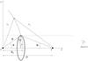 |
Fig. 1 Schematic diagram showing the interaction of two spherical winds that move radially away from the stars. Source 1 of the wind with velocity v1 is located at the origin of the coordinate system, and source 2 of the wind with velocity v2 at a distance D along the symmetry axis. The shape of the layer where the winds collide (at R0 along the symmetry axis) is given by the curve R(θ). The angles θ and θ1 are measured from the positions of the stars to the intersection point between a line of sight (with impact parameter r) and the layer. We assume azimuthal symmetry (no dependence on angle φ). The observer is located in the orbital plane along the z-axis of symmetry. |
The pressure within the shell just behind each shock can be written in terms of the preshock density, and the velocity component normal to the shell. The normal vector to the surface of the shell can be obtained from the gradient of the function F = r′ − R(θ), where r′ is the radial coordinate, and the bow shock is described by F = 0. In this way,  , where ∇ denotes the vector differential operator gradient in spherical coordinates (see Wilkin 1997). For isotropic outflows ∂R/∂φ = 0 (see Eq. (1)), and then
  (3)where
  and
and  are unit vectors measured along the directions R and θ, respectively.
On the other hand, the velocity vectors of the stellar winds are given by  (4)and
  (5)From Eqs. (3)–(5) it follows that the normal component at every point (R,θ,φ) of the pre-shock velocity of the stellar winds are obtained by
  As a result, the pressure within the thin shell just behind each shock front can be written as
  (8)and
 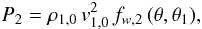 (9)where we have used the wind parameters ρ1,0 and
  at the stagnation point R0 to nondimensionalize the equations, and
 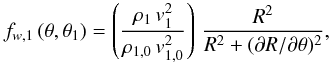 (10)and
 ![Mathematical equation: \begin{eqnarray} f_{w,2}\,(\theta,\theta_1)&=& \left({{\rho_{2}\, v_{2}^{2}} \over{\rho_{1,0}\, v_{1,0}^{2}}}\right)\, \nonumber \\ &&\quad \times {{{[R\,\mbox{cos}\,(\theta + \theta_1) + (\partial R/ \partial \theta)\, \mbox{sin}\,(\theta + \theta_1)]}^2} \over{R^2 + (\partial R/ \partial \theta)^2}}, \label{eq11} \end{eqnarray}](/articles/aa/full_html/2011/07/aa15988-10/aa15988-10-eq50.png) (11)where ρ1 and ρ2 are the preshock densities of the stellar winds.
(11)where ρ1 and ρ2 are the preshock densities of the stellar winds.
2.1. The emission measure of the thin shell
Let l be a longitude-coordinate measured inwards from the wind shock of source 2 and perpendicular to the thin shell (as shown in Fig. 2). Then, the shock fronts are located at l = 0 and l = h, where h is the position-dependent thickness of the shell. We assume that the post-shock gas is well mixed, so that it flows along the shell at a velocity v, which is independent of l. If the whole flow is photoionized and approximated as an isothermal flow, the pressure as a function of the parameter l can be calculated from the hydrostatic equation  (12)where
  (with cs being the isothermal sound speed), and the centrifugal acceleration g = v2/Rc, with Rc the radius of curvature of the thin shell. Integrating Eq. (12) with the boundary condition P2 = P(l = 0), we obtain
 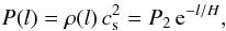 (13)where
  is the scale height parameter of pressure (or density). It follows from Eq. (13) that the surface density is given by
 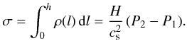 (14)Using Eqs. (13) and (14), we can now calculate the emission measure of the thin shell,
  (15)where
  is the average mass per particle of the photoionized gas, μ the mean atomic weight per electron, and mp the mass of the proton.
 |
Fig. 2 Schematic diagram showing a thin shell (limited by two shock fronts) resulting from the interaction of two stellar winds. The shocked gas flows along the shell at a velocity v and has a surface density σ. The coordinate l is measured inwards from the wind shock of source 2, normal to the locus of the thin shell. |
Equation (15) gives the emission measure of the thin shell in terms of its surface density. Next, we must obtain the surface density as a function of position on the shell. We first note that the shocked gas can be described as a flow of streamlines with constant azimuthal angle φ. The mixing of the two shocked winds is assumed to be instantaneous, so that the flow will have a unique velocity v at any location with in the shell. The mass (per unit time) ΔṀ flowing along a ring of radius r of the layer is then given by  (16)which must be equal to the mass injection rate (into the same solid angle) of the stellar winds, that is,
  (17)with
  (18)Based on considerations of linear momentum conservation, it can be shown that the velocity along the shell (see also Cantó et al. 1996; 2005) can be written as
  (19)where the functions fr (θ,θ1) and fz (θ,θ1) are deduced from r-momentum and z-momentum (being r and z the directions of the cylindrical radius and the symmetry axis, respectively), and are given by
 ![Mathematical equation: \begin{eqnarray} f_r(\theta, \theta_1)= {{1}\over{2}}\,\left[\theta - \mbox{sin}\,\theta\, \mbox{cos}\,\theta + {{1}\over{\beta}}\, (\theta_1 - \mbox{sin}\,\theta_1\,\mbox{cos}\,\theta_1)\right], \label{eq20} \end{eqnarray}](/articles/aa/full_html/2011/07/aa15988-10/aa15988-10-eq79.png) (20)and
(20)and ![Mathematical equation: \begin{eqnarray} f_z(\theta, \theta_1)= {{1}\over{2}}\,\left[ \mbox{sin}^2\,\theta\, - {{1}\over{\beta}}\,\mbox{sin}^2\,\theta_1\ \right]\,. \label{eq21} \end{eqnarray}](/articles/aa/full_html/2011/07/aa15988-10/aa15988-10-eq80.png) (21)Substitution of Eqs. (17) − (21) into Eq. (16) gives the surface density,
(21)Substitution of Eqs. (17) − (21) into Eq. (16) gives the surface density,  (22)where σ0 = ṁ1/(2πβDv1) and
  (23)Finally, it follows from Eq. (15) that the emission measure of the thin shell (as a function of position) is given by
 ![Mathematical equation: \begin{eqnarray} EM(\theta, \theta_1)= EM_0\,f_{\sigma}(\theta, \theta_1) \,[f_{w,1}\,(\theta,\theta_1) + f_{w,2}\,(\theta,\theta_1)], \label{eq24} \end{eqnarray}](/articles/aa/full_html/2011/07/aa15988-10/aa15988-10-eq85.png) (24)with
(24)with 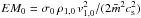 .
.
2.2. Predicted thermal radio emission from a binary system
To calculate the radio-continuum emission from the whole system, it is necessary to compute the total optical depth along each line of sight, which will have the contribution from the stellar winds and also from the thin shell. Then we estimate the intensity emerging from each direction and calculate the flux by integrating the intensity over the solid angle.
Given the emission measure EM(θ,θ1) of the shocked layer (Eq. (24)), the optical depth perpendicular to the WCR is calculated by τWCR, ⊥ (θ,θ1) = EM(θ,θ1) χ(ν), where χ(ν) = 8.436 × 10⁻⁷ ν-2.1 with the frequency ν in Hz (for an electron temperature Te = 104 K). By defining a critical frequency, such that 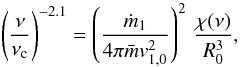 (25)it can be shown from Eq. (24) that
 ![Mathematical equation: \begin{eqnarray} \tau_{{\rm WCR},\perp}(\theta, \theta_1)&=& \left({{\nu}\over{\nu_{\rm c}}}\right)^{-2.1} \,\left({{v_{1,0}}\over{c_{\rm s}}}\right)^2 \nonumber \\ &&\quad\times\left(\,{{1}\over{\beta \tilde D}}\right)\, f_{\sigma}(\theta, \theta_1) \,[f_{w,1}\,(\theta,\theta_1) + f_{w,2}\,(\theta,\theta_1)], \label{eq26} \end{eqnarray}](/articles/aa/full_html/2011/07/aa15988-10/aa15988-10-eq92.png) (26)where
(26)where  . For a line of sight intersecting the thin shell at an angle
  from the normal (being
 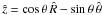 ), the optical depth is then given by
 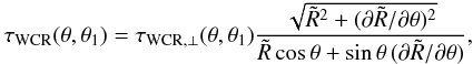 (27)where
  is in units of R0.
Let us now calculate the contribution of the unshocked stellar winds to the optical depth. Consider a line of sight that intersects the thin shell at a point  , as shown in Fig. 1. According to Panagia & Felli (1975) and Wright & Barlow (1975), the optical depth along the line of sight of the wind source located at z = 0 is obtained by
 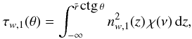 (28)where
  (29)where
  (=
(=  ) is the number density of the flow at the stagnation point. From Eqs. (25)–(29), it follows that
  (30)with
 ![Mathematical equation: \begin{eqnarray} I_{w,1}(\theta)= {{1}\over{2 \tilde{r}^3}}\, \left[{{\pi}\over{2}} + {{\mbox{ctg}\,\theta} \over{\mbox{ctg}^2\,\theta + 1}} + \theta\,\right]\,. \nonumber \end{eqnarray}](/articles/aa/full_html/2011/07/aa15988-10/aa15988-10-eq106.png) Analogously, the optical depth of the wind source located at z = D is calculated by
Analogously, the optical depth of the wind source located at z = D is calculated by  (31)where
 ![Mathematical equation: \begin{eqnarray} n_{w,2}(\tilde{z})= n_{2,0}\, {{1}\over{[\tilde{z}-\tilde{D}]^2 + \tilde{r}^2}}, \label{eq32} \end{eqnarray}](/articles/aa/full_html/2011/07/aa15988-10/aa15988-10-eq109.png) (32)where
(32)where  (=
(=  ) is the number density of the wind at the stagnation point. Substitution of (32) into Eq. (31) gives
 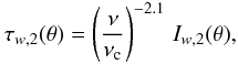 (33)with
 ![Mathematical equation: \begin{eqnarray} I_{w,2}(\theta)&=& \left({{\dot{m_2}\,v_1}\over{\dot{m_1}\,v_2}}\right)^2 {{1}\over{2 \tilde{r}^3}}\, \Bigg[{{\pi}\over{2}} - {{(\tilde{r}\,\mbox{ctg}\,\theta - \tilde{D})\,\tilde{r}} \over{\tilde{r}^2 + (\tilde{r}\,\mbox{ctg}\,\theta - \tilde{D})^2}} \nonumber \\ &&\quad- {\rm arctg}\,\left({{\tilde{r}\,\mbox{ctg}\,\theta - \tilde{D}}\over{\tilde{r}}}\right)\,\Bigg]. \nonumber \end{eqnarray}](/articles/aa/full_html/2011/07/aa15988-10/aa15988-10-eq113.png) We assumed that the system is far enough (D ≪ L, being L the distance to the observer) so that the lines of sight intersecting the central stars can be ignored. Then, the radio-continuum flux from the colliding wind binary can be calculated by
We assumed that the system is far enough (D ≪ L, being L the distance to the observer) so that the lines of sight intersecting the central stars can be ignored. Then, the radio-continuum flux from the colliding wind binary can be calculated by ![Mathematical equation: \begin{eqnarray} S_{\nu}= 2 \pi B_{\nu}\,\left({{R_0}\over{L}}\right)^2\, \int_{0}^{\tilde{r}(\theta_{\infty})} [1 - \mbox{e}^{-\tau(\theta,\theta_1)}]\, \tilde{r}\,{\rm d}\tilde{r}, \label{eq34} \end{eqnarray}](/articles/aa/full_html/2011/07/aa15988-10/aa15988-10-eq116.png) (34)where τ(θ,θ1) = τWCR(θ,θ1) + τw,1(θ) + τw,2(θ) is the total optical depth along the line of sight, Bν (= 2kTν2/c2 with k the Boltzmann’s constant, and c the light speed) is the Planck function in the Rayleigh-Jeans approximation, and
(34)where τ(θ,θ1) = τWCR(θ,θ1) + τw,1(θ) + τw,2(θ) is the total optical depth along the line of sight, Bν (= 2kTν2/c2 with k the Boltzmann’s constant, and c the light speed) is the Planck function in the Rayleigh-Jeans approximation, and  is the impact parameter at the asymptotic angle θ∞ (corresponding to R → ∞) of the thin shell, which can be found from
 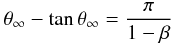 (see Cantó et al. 1996). Defining the parameter
 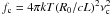 , we finally obtain
 ![Mathematical equation: \begin{eqnarray} S_{\nu}&= &f_{\rm c} \,\left({{\nu}\over{\nu_{\rm c}}}\right)^{2}\Bigg[ \int_{0}^{\theta_{\infty}} [1 - \mbox{e}^{-\tau(\theta,\theta_1)}]\, \tilde{R}^2(\theta)\,\mbox{sin}\,\theta\,\mbox{cos}\,\theta\,{\rm d}\theta \nonumber \\ &&\quad + \int_{0}^{\theta_{\infty}} [1 - \mbox{e}^{-\tau(\theta)}]\, \tilde{R}(\theta)\,\mbox{sin}^2\,\theta\, (\partial \tilde{R}/ \partial \theta)\,{\rm d}\theta\, \Bigg]\,. \label{eq35} \end{eqnarray}](/articles/aa/full_html/2011/07/aa15988-10/aa15988-10-eq127.png) (35)Equation (35) represents an self-similar solution for the free-free radiation from colliding stellar winds from massive binary systems.
(35)Equation (35) represents an self-similar solution for the free-free radiation from colliding stellar winds from massive binary systems.
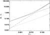 |
Fig. 3 Predicted free-free emission from a colliding wind binary. We have adopted the parameters v1 = 103 km s-1, ṁ1 = 1.25 × 10⁻⁵ M⊙ yr-1, and v2 = 103 km s-1, ṁ2 = 5 × 10⁻⁵ M⊙ yr-1 for the wind sources. The binary separation is set to D = 4 AU. The dotted and dashed lines represent the fluxes (∝ ν0.6) from the wind sources 1 and 2 (see also Fig. 1), respectively. The intrinsic thermal emission from the WCR (dot-dashed line) and the total emission (solid line) from the binary system are also shown. The behavior of the curves is described in the main text. |
We apply the model for computing the emission from a colliding wind binary using stellar wind parameters similar to those from a typical WR+O binary system. That is, we have adopted v1 = 103 km s-1, ṁ1 = 1.25 × 10⁻⁵ M⊙ yr-1 for the O type star, and for the WR component, v2 = 103 km s-1, ṁ2 = 5 × 10⁻⁵ M⊙ yr-1. In addition, we have assumed a separation D = 4 AU between the stars (so that the WCR is radiative; see Sect. 3). The result is shown in Fig. 3. It shows the contribution to the total radio emission of the unshocked stellar winds and the WCR. As expected for ionized stellar envelopes (see Sect. 1), the flux densities from the stellar winds increases as ~ν0.6. However, deviation from the expected 0.6 value of the spectral index at high frequencies is observed from the emission of the wind source 1. This is probably due to the presence of the WCR inside the optically thick region of the wind. We note that as ν increases the emission from the WCR becomes more important. The intrinsic flux density from the WCR shows a spectral index of ~1.1, consistent with the numerical models (in massive O+O type binary stars) developed by Pittard (2010). At low frequencies, the total flux density grows as Sν ~ ν0.6 approaching the emission from the stronger wind. On the other hand, at higher frequencies, the radio spectrum from the system approaches the flux density from the WCR (Sν ~ ν1.1).
3. Thermal radio-continuum emission from colliding wind binaries
As mentioned in Sect. 1, radio observations (e.g. Moran et al. 1989; Dougherty et al. 2000; Montes et al. 2009) and theoretical models (see, for instance, Dougherty et al. 2003; Pittard et al. 2006; Pittard 2000) of massive binary stars have revealed strong shocks formed in the wind-wind interaction zone. These shocks emit radio-continuum radiation consistent with thermal emission that may produce variations in the expected flux densities and spectral indices from ionized stellar winds. In this section, we apply the model of colliding-wind binary systems developed in Sect. 2 by adopting different wind parameters of the components. Our model assumes strong radiative shocks which collapse onto a thin shell, so that the width of the WCR can be neglected. We investigate the contribution of the WCR to the thermal radiation from colliding-wind binaries, and the effect of the binary separation on the radio spectrum.
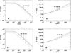 |
Fig. 4 Optical depth τWCR(43 GHz) of the WCR as a function of impact parameter r (left panels), and the predicted flux density Sν at radio frequencies (right panels) for the models of Table 1. In top panels, the dot-dashed, solid and dotted lines represent the optical depth and the radio spectrum from the models B1, B2, and B3, respectively. In bottom panels, the corresponding values of models B2, B4, and B5 are shown by the solid, dot-dashed, and dotted lines, respectively. The physical description of the plots are given in the text. |
Stevens et al. (1992) investigated the collision of stellar winds in early-type binary systems. They studied the role of radiative cooling in the structure and dynamics of colliding wind binaries. In this work, the importance of cooling in a particular system is quantified using the cooling parameter χ (≈  , where v3 the wind velocity in units of 103 km s-1, dAU the distance to the contact discontinuity in units of AU, and Ṁ5 is the mass loss rate in units of 10-5 M⊙ yr-1), defined as the ratio of the cooling time of the shocked gas to the escape time from the intershock region. For models with χ ≥ 1, the postshock flow can be assumed to be adiabatic, while it is roughly isothermal for models with χ ≪ 1. Numerical simulations by these authors show that the cooling result in the formation of a thin dense shell, confined by isothermal shocks, as χ drops below unity. Antokhin et al. (2004) have also investigated the narrowness of the cooling layer using the ratio l0/R (where l0 is the cooling length and R the radius from the star source), which is closely related to the above parameter χ. These authors show that the ratio l0/R can serve as well to distinguish between adiabatic and radiative shocks, with l0/R > 1 implying an adiabatic shock and l0/R < 1 a radiative one.
Nonetheless, radiative pressure that moderates the wind-wind collision may be important in close hot-star binaries. An initial analysis was developed by Stevens & Pollock (1994), who investigated the dynamics of colliding winds in massive binary systems. They show that, in close binaries, the radiation of a luminous star inhibits the initial acceleration of the companion’s wind towards the stagnation point. These radiative forces result in lower velocities than those expected in single-star models moderating the wind collision. In other work, Gayley et al. (1997) investigated the potential role of the radiative braking effect, whereby the primary wind is decelerated by radiation pressure as it approaches the surface of the companion star. These authors conclud that radiative braking must have a significant effect for wind-wind collision in WR+O binaries with medium separations (D < 0.5 AU). Furthermore, Parkin & Pittard (2008) carried out 3D hydrodynamical simulations of colliding winds in binary systems. They shows that the shape of the WCR is deformed by Coriolis forces into spiral structures by the motion of the stars. The shape of the shock layer is more deformed in systems with eccentric orbits. In addition, Pittard (2010) developed 3D hydrodynamical models of massive O+O star binaries for computing the thermal radio to submillimeter emission. In this work, flux and spectral index variations with orbital phase and orientation of the observer (from radiative and adiabatic systems) are investigated. These authors found strong variations in eccentric systems caused by dramatic changes to the physical properties (density and temperature) of the WCR, which is radiative (optically thick) at periastron, but adiabatic (optically thin) at apastron.
3.1. The predicted radio emission from radiative shocks in colliding wind binaries
Here, we present analytic predictions of the thermal spectra at radio frequencies from different radiative models, which satisfy the condition of radiative shocks (χ < 1) for the WCR. We have estimated the value of χ for each shock of the WCR. In Table 1, we list the different scenarios of colliding wind binaries that we have studied in this paper. In models B1 − B3, we have assumed identical wind sources (β = 1) in order to investigate the effect of the binary separation. On the other hand, in models B2, B4, and B5, we have assumed different wind momentum ratios for the binary systems, while the distance between the components is unchanged. In models B4 and B5, we indicate the highest value of χ for each system. These models for the radio emission from colliding wind binaries are presented in Fig. 4. We show the optical depth of the WCR as functions of the impact parameter r (left panels) and the predicted flux density at radio frequencies (right panels). Top panels show the results of our Models B1 − B3, while the models B2, B4, and B5 are shown in the bottom panels. All models are calculated for an observer located in the orbital plane along the symmetry axis (which corresponds to a system with an inclination angle i = 90° with the most powerful stellar wind in front, as shown in Fig. 1).
First, we observe that, for low-impact parameters (r/R0 ≤ 1), the optical depth τWCR(43 GHz) of the WCR (Fig. 4a) does not depend on the value of r and scales as D-3. On the other hand, for higher impact parameters (r/R0 ≫ 1), τWCR(43 GHz) ∝ r-5 in all models. At a given line of sight, we also note that, in this limit, the optical depth increases as D2. The transition impact parameter is r ∝ R0 (see, also, Appendix A). This behavior of the optical depth (and therefore of the emission measure of the thin shell) can be explained as follows (see Figs. A.1 and A.2). We consider a given impact parameter r and vary the binary separation. For systems with r/R0 ≫ 1 (τs ∝ r-5), as the binary separation (and therefore R0) increases, the ratio r/R0 decreases. The normal components of the shock velocities (for the two shock fronts that bound the WCR) increase for higher values of R0, which result in higher pressures within the shocked layer (Eqs. (8) and (9)). Thus, both the emission measure (Eq. (15)) and the optical depth (Eq. (27)) of the thin shell increase. On the other hand, for systems with r/R0 ≪ 1 (τs ≠ τs [r/R0 ] ), as R0 increases the preshock densities (for the two shock fronts of the WCR) decreases, which result in lower pressures within the shocked layer. Consequently, the emission measure and the optical depth of the WCR diminish.
Parameters of the colliding winds.
Second, we show the predicted flux density at radio frequencies for models B1 − B3 (Fig. 4b). We note that, at frequencies ν > 1 GHz, as the binary separation increases, the emission from the binary becomes more important. In order to explain this behavior of the spectrum, we investigated the emission from the shocked layer as a function of the impact parameter r (see Sect. A.3 of Appendix A). Our results are presented in Fig. A.3. We show that the main contribution to the flux comes from the optically thick region of the shell, so the emission from the optically thin region can be neglected. In addition, our model predicts that the emission from an optically thick WCR (which is bounded by radiative shocks) scales as Sν ∝ D4/5 (see Fig. A.4). This result contrasts with the inverse dependence with the binary separation described by Pittard et al. (2006) for an adiabatic and optically thin WCR, where the emission is expected to scale as D-1.
Finally, as mentioned above, the effect of varying the wind momentum ratio β on the value of τWCR(43 GHz), and the total spectrum, is investigated from models B2, B4, and B5 (bottom panels of Fig. 4). As we expected from Eqs. (26) − (27), it can be observed that the optical depth of the WCR increases with the mass loss rate ṁ1 of the secondary component (Fig. 4c). In addition, Fig. 4d shows the predicted thermal radio spectra from these models. The plots show how sensitive our analytic model is to the wind momentum radio, β. We note that, at high frequencies, the total flux density Sν increases with the parameter β.
4. Comparison with observations
As we mention in previous sections, the model presented in this paper assumes a thin shell approximation for the colliding wind region. In the presence of efficient cooling (χ < 1), the WCR is confined by radiative shocks, which are expected in close binaries. Consequently, we investigate the emission from short period (< 1 yr) WR+O systems calculated with the analytic model developed in Sect. 2. Besides, radiative breaking can be important for binaries with a medium separation D < 100 R⊙ (orbital periods ~15 days), which prevents the applicability of our model for systems with shorter periods.
Recently, Montes et al. (2009) have reported observations of the flux density and spectral indices for the close systems WR 98 113, 138, and 141. In this section, we apply the analytical model to the binaries WR 98 and WR 113 and compare them with observations. Table 2 lists the adopted stellar parameters of these sources in our colliding wind model, which suggest the presence of radiative shocks in the wind-wind interaction zone. We indicate the highest value of χ for each binary system. We indicate the highest value of χ for each binary system. We show that the contribution of the WCR to the total emission gives a possible explanation to the observations.
Wind parameters of colliding wind models.
WR 98. This close binary has been identified as a double line binary (WN7o/WC+O8-9) with an orbital period, P = 47.8 days (Gamen & Niemela 2002). Abbott et al. (1986) classified WR 98 as a nonthermal radio source. Recently, multi-wavelength observations (from 5 to 23 GHz) of this source have revealed that the spectral index changed from ~0.26 to ~0.64 in a period of time of ~15 days (Montes et al. 2009). This behavior was interpreted as indicating a binary influence over the radio spectrum, possibly from a variable nonthermal contribution that is absorbed at certain orbital phases, turning the spectrum into a “thermal state”. The stellar parameters of this binary indicate that a radiative WCR (χ ~ 0.6) is formed within this system.
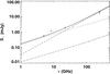 |
Fig. 5 Comparison between our model and the flux densities at 5, 8.4, 23 and 250 GHz (“+” sign; uncertainty in the flux measurements are given by the length of the bars) of the binary system WR 98 obtained by Montes et al. (2009) and Altenhoff et al. (1991), respectively. We have assumed the stellar wind parameters ṀWR = 3.0 × 10⁻⁵ M⊙ yr-1, vWR = 1200 km s-1, ṀO = 4.0 × 10⁻⁶ M⊙ yr-1, and vO = 1800 km s-1. The stars are separated by a distance D ~ 0.5 AU. The dotted and dashed lines represent the fluxes (∝ ν0.6) from the winds of the WR and O type stars, respectively. The radiation from the WCR (dot-dashed line) and the total flux density (solid line) from the binary source are also shown. The physical description of the plot is given in the text. |
We applied the model to the binary system WR 98 to investigate if a thermal component of emission from the WCR is able to contribute significantly to the total spectrum. Our results from the model are compared with the observations at the thermal state (α ~ 0.64) reported by Montes et al. (2009). We assumed for the WR star a mass loss rate ṀWR = 3.0 × 10⁻⁵ M⊙ yr-1 (upper limit derived from radio observations at the thermal phase at 8.4 GHz when α ~ 0.64; Montes et al. 2009), and an ejection velocity vWR = 1200 km s-1 (Eenens & Williams 1994). The best fit to the observations was found from the O star parameters ṀO = 4.0 × 10⁻⁶ M⊙ yr-1 and vO = 1800 km s-1. We have assumed a mean atomic weight per electron μ = 4.2 and an average ionic charge Z = 1.1 for the WR wind, and μ = 1.5 and Z = 1 for the O star (which are typical values for O-type stars; see Bieging et al. 1989). Using Eq. (19) in Cantó et al. (1996) and considering that most of the emission from the WCR arise from impact parameters, r, such that θ < θ∞ (see Table 2), we can estimate the ratio of mass entering into the WCR from the WR stellar wind, to that from the O star, ΔMWR/ΔMO > 0.75. Thus, we assume that the material within the shock is mainly composed of what comes from the strongest wind, assuming the same values of μ and Z for the shocked material as those used for the WR wind. From the value of asini ~ 100 R⊙, (where a is the semi-major axis and i is the inclination angle of the orbit) determined by Gamen & Niemela (2002), we assume D ~ 0.5 AU for the binary separation, which is the maximum value for a (when i ~ 90°). Since this value represents an upper limit for D and because the geometric configuration represents the WR stellar wind in front of the O star, we are determining the minimum expected for the WCR thermal contribution.
In Fig. 5, we show the predicted spectrum from WR 98 system. Observational data (S5 GHz = 0.58 ± 0.06 mJy, S8.4 GHz = 1.18 ± 0.05 mJy, and S23 GHz = 1.94 ± 0.15 mJy) by Montes et al. (2009) are also plotted. It can be seen that our model predicts an increase in the flux density at high frequencies, which results in steeper spectral indices than the expected 0.6 value of the stellar winds. Also the WCR emission becomes comparable to that from the WR wind at ~70 GHz, and at a frequency of 250 GHz, the shock layer produces an excess of emission of a factor >2 over the value expected for the WR wind (8 mJy). To test this prediction of the model at higher frequencies, we included the flux density S250 GHz = 19 ± 5 mJy measured by Altenhoff et al. (1991), which seems to agree with the 22 mJy predicted for the total flux density at 250 GHz. Furthermore, the spectral index of the WCR emission, αWCR ~ 1.2, is similar to what is derived from the observations at this frequency range, α22.5 − 250 GHz ~ 0.95.
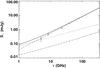 |
Fig. 6 Comparison between our model and the flux densities at 5, 8.4, 23 GHz (“+” sign; uncertainty in the flux measurements are given by the length of the bars) of the binary system WR 113 obtained by Montes et al. (2009). We have assumed the stellar wind parameters ṀWR = 2.0 × 10⁻⁵ M⊙ yr-1, vWR = 1700 km s-1, ṀO = 0.4 × 10⁻⁵ M⊙ yr-1, and vO = 1800 km s-1. The stars are separated by a distance D ~ 0.6 AU. The dotted and dashed lines represent the fluxes (∝ ν0.6) from the winds of the WR and O type stars, respectively. The radiation from the WCR (dot-dashed line) and the total flux density (solid line) from the binary source are also shown. The physical description of the plot is given in the text. |
WR 113. This source was detected at radio frequencies (8.4 GHz) for first time by Cappa et al. (2004). The period of this spectroscopic binary (WC8+O8-9) is P = 29.7 days (Niemela et al. 1996). Recently, simultaneous multifrequency observations (from 5 to 23 GHz) of WR 113 by Montes et al. (2009) showed an spectral index α ~ 1.06. We have modeled this binary adopting the wind parameters ṀWR = 2.0 × 10⁻⁵ M⊙ yr-1 (Lamontagne et al. 1996) and vWR = 1700 km s-1 (van der Hucht et al. 2001) for the WR star, and ṀO = 0.4 × 10⁻⁵ M⊙ yr-1 and v0 = 1800 km s-1 for the O type component, separated by a distance D = 0.6 AU (from the value asini = 129 R⊙, and i ~ 70 determined by Lamontagne et al. 1996). We assume a mean atomic weight per electron μ = 4.7 and an average ionic charge Z = 1.1 for the stellar wind of the WR wind (from Cappa et al. 2004), and μ = 1.2 and Z = 1 for the O star. As in the case of WR 98, we assumed that the shock is mainly composed of material from the WR wind (ΔMWR/ΔMO > 0.65), and the same μ and Z values were used. Figure 6 shows the predicted spectrum by the model, as well as observational data (S5 GHz = 0.22 ± 0.03 mJy, S8.4 GHz = 0.47 ± 0.04 mJy, and S23 GHz = 1.27 ± 0.07 mJy) from the WR 113 system by Montes et al. (2009). We note from the figure that the contribution of the WCR starts to dominate the emission from the system at a lower frequency (ν ~ 9 GHz) than in the case of WR 98, mainly because the flux density from the WR star is ~3 times lower than for WR 98. At a frequency of 250 GHz, the flux density from the thin shell becomes a factor of ~6 greater that the expected value from the unshocked winds. Observations at such high frequencies are required in order to verify the high spectral indices predicted by our model.
From our model, we have shown that a thermal contribution from the WCR in WR 98 and WR 113 is likely to be detected at high frequencies. However, as we pointed out, we can only present a lower limit for this contribution, owing to the uncertainty of parameters such as the binary separation, D. On the other hand, Pittard (2010) have investigated the variability in the flux density (from radiative systems) due to the orbital motion of the stars and orientation of the observer. The configuration adopted in our model (with an inclination angle of 90° and orbital phase ~0) corresponds to the minimum contribution to the total thermal emission expected from radiative shocks in binary systems with an inclination angle ~90°. In this way, the excess of emission predicted here is expected to be variable and modulated by the orbit motion. WR 98 was reported as a variable source by Montes et al. (2009), changing its spectral index from ~0.26 to ~0.64 in a period of ~15 days. Although the flat spectral index (~0.26) resembles the one predicted by Pittard et al. (2006) for an adiabatic shock, this close system is likely to be radiative, and such behavior was explained as result of a nonthermal contribution escaping the absorption. On the other hand, for WR 113 there are no observations at high frequencies or clear evidence of variability to support the contribution predicted here; therefore, high-frequency observations are required to confirm it.
5. Summary and conclusions
In this paper, we have presented an analytical model for calculating the thermal contribution at radio frequencies from the WCR in massive binary systems. The strong stellar winds of both components collide and form the WCR (bounded by two shock fronts) between the stars, which emits both thermal (free-free) and nonthermal (synchrotron) radiation. In particular, the nonthermal component is expected to be highly absorbed in close binaries, so the thermal flux must be the dominant contributor. In addition, particle acceleration should not occur if the shocks are collisional such as in short period systems where the gas density is high.
Based on considerations of linear and angular momentum conservation, we developed a formulation for calculating the emission measure of the WCR, from which simple predictions of the thermal emission can be made. We assumed that the WCR is bounded by radiative shocks, so that the width of the WCR can be neglected and the wind-wind interaction zone can be approximated as a thin shell. Since highly radiative shocks are expected to occur in short period systems, we assumed different scenarios of colliding wind close binaries. Using typical parameters of massive WR+O binaries, we showed that the compressed layer emits free-free radiation that plays a very substantial role in the emission from the whole system. The radio-continuum spectrum obtained by our model clearly deviates from the behavior Sν ∝ ν0.6 predicted by the standard stellar wind model.
In previous models (Pittard et al. 2006), the expected thermal emission from binary systems where the WCR remains optically thin (confined by adiabatic shocks) was investigated. In this case, the flux density scales as D-1; consequently, the emission from the WCR increases as the binary separation decreases. In this work, we study the thermal radiation from systems where the WCR is highly radiative. The effects of the binary separation and the wind momentum ratio on the total spectrum are investigated. Our model’s results show that the relative contribution of the WCR to the total emission mainly arises from the optically thick region of the layer, which flux density scales as D2 (where D is the stellar separation). Thus, the impact of the WCR to the total spectrum (in contrast to the optically thin case) becomes more important as the binary separation increases (until the WCR becomes optically thin).
Finally, we applied the analytical model to massive binaries, and calculated the thermal radio-continuum emission from the short-period WR+O systems, WR 98 and WR 113. Assuming a set of wind parameters consistent with observations of these sources, we find that the WCR must be confined by radiative shocks, and so the thin shell approximation can be applied. In both sources, the compressed layer generates thermal radiation that produces (at high frequencies) an excess of emission over the expected values from the stellar winds. Comparison with recent observations (by Montes et al. 2009) from these sources showed that our model can satisfactorily reproduce the flux densities and spectral indices.
Acknowledgments
G.M. acknowledges financial support from a CSIC JAE-PREDOC fellowship. R.F.G. has been partially supported by DGAPA (UNAM) grant IN117708. J.C. acknowledges support from CONACyT grant 61547. This research was partially supported by the Spanish MICINN through grant AYA2009-13036-CO2-01. The authors acknowledge the anonymous referee for the helpful comments that improved the content and presentation of the paper.
References
- Abbott, D. C., Beiging, J. H., Churchwell, E., & Torres, A. V. 1986, ApJ, 303, 239 [NASA ADS] [CrossRef] [Google Scholar]
- Altenhoff, W. J., Thum, C., & Wendker, H. J. 1994, A&A, 281, 161 [NASA ADS] [Google Scholar]
- Antokhin, I. I., Owocki, S. P., & Brown, J. C. 2004, ApJ, 611, 434 [NASA ADS] [CrossRef] [Google Scholar]
- Bieging, J. H., Abbott, D. C., & Churchwell, E. B. 1989, ApJ, 340, 518 [NASA ADS] [CrossRef] [Google Scholar]
- Cantó, J., Raga, A. C., & Wilkin, F. P. 1996, ApJ, 469, 729 [NASA ADS] [CrossRef] [Google Scholar]
- Cantó, J., Raga, A. C., & González, R. 2005, Rev. Mex. Astron. Astrofis., 41, 101 [Google Scholar]
- Cappa, C., Goss, W. M., & van der Hucht, K. A. 2004, AJ, 127, 2885 [NASA ADS] [CrossRef] [Google Scholar]
- Dougherty, S. M., & Williams, P. M. 2000, MNRAS, 319, 1005 [NASA ADS] [CrossRef] [Google Scholar]
- Dougherty, S. M., Williams, P. M., & Pollacco, D. L. 2000, MNRAS, 316, 143 [NASA ADS] [CrossRef] [Google Scholar]
- Dougherty, S. M., Pittard, J. M., Kasian, L., et al. 2003, A&A, 409, 217 [NASA ADS] [CrossRef] [EDP Sciences] [Google Scholar]
- Eenens, P. R. J., & Williams, P. M. 1994, MNRAS, 269, 1082 [NASA ADS] [Google Scholar]
- Eichler, D., & Usov, V. 1993, ApJ, 402, 271 [NASA ADS] [CrossRef] [Google Scholar]
- Gamen, R. C., & Niemela, V. S. 2002, New Astron., 7, 511 [NASA ADS] [CrossRef] [Google Scholar]
- Gayley, K. G., Owocki, S. P., & Cranmer, S. R. 1997, ApJ, 475, 786 [NASA ADS] [CrossRef] [Google Scholar]
- González, R. F., & Cantó, J. 2008, A&A, 477, 373 [NASA ADS] [CrossRef] [EDP Sciences] [Google Scholar]
- Kenny, H. T., & Taylor, A. R. 2005, ApJ, 619, 527 [NASA ADS] [CrossRef] [Google Scholar]
- Lamontagne, R., Moffat, A. F. J., Drissen, L., Robert, C., & Matthews, J. M. 1996, AJ, 112, 2227 [NASA ADS] [CrossRef] [Google Scholar]
- Leitherer, C., & Robert, C. 1991, ApJ, 377, 629 [NASA ADS] [CrossRef] [Google Scholar]
- Luo, D., McCray, R., & Mac Low, M.-M. 1990, ApJ, 362, 267 [NASA ADS] [CrossRef] [Google Scholar]
- Niemela, V. S., Morrell, N. I., Barba, R. H., & Bosch, G. L. 1996, Rev. Mex. Astron. Astrofis. Conf. Ser., 5, 100 [NASA ADS] [Google Scholar]
- Nugis, T., Crowther, P. A., & Willis, A. J. 1998, A&A, 333, 956 [NASA ADS] [Google Scholar]
- Monnier, J. D., Greenhill, L. J., Tuthill, P. G., & Danchi, W. C. 2002, ApJ, 566, 399 [NASA ADS] [CrossRef] [Google Scholar]
- Montes, G., Pérez-Torres, M. A., Alberdi, A., & González, R. F. 2009, ApJ, 705, 899 [NASA ADS] [CrossRef] [Google Scholar]
- Moran, J. P., Davis, R. J., Spencer, R. E., Bode, M. F., & Taylor, A. R. 1989, Nature, 340, 449 [NASA ADS] [CrossRef] [Google Scholar]
- Panagia, N., & Felli, M. 1975, A&A, 39, 1 [NASA ADS] [Google Scholar]
- Parkin, E. R., & Pittard, J. M. 2008, MNRAS, 388, 1047 [NASA ADS] [CrossRef] [Google Scholar]
- Pittard, J. M. 2009, MNRAS, 396, 1743 [NASA ADS] [CrossRef] [Google Scholar]
- Pittard, J. M. 2010, MNRAS, 403, 1633 [NASA ADS] [CrossRef] [Google Scholar]
- Pittard, J. M., Stevens, I. R., Corcoran, M. F., et al. 2000, MNRAS, 319, 137 [NASA ADS] [CrossRef] [Google Scholar]
- Pittard, J. M., Dougherty, S. M., Coker, R. F., O’Connor, E., & Bolingbroke, N. J. 2006, A&A, 446, 1001 [NASA ADS] [CrossRef] [EDP Sciences] [Google Scholar]
- Stevens, I. R. 1995, MNRAS, 277, 163 [NASA ADS] [Google Scholar]
- Stevens, I. R., & Pollock, A. M. T. 1994, MNRAS, 269, 226 [NASA ADS] [CrossRef] [Google Scholar]
- Stevens, I. R., Blondin, J. M., & Pollock, A. M. T. 1992, ApJ, 386, 265 [NASA ADS] [CrossRef] [Google Scholar]
- Williams, P. M., van der Hucht, K. A., Pollock, A. M. T., et al. 1990, MNRAS, 243, 662 [NASA ADS] [Google Scholar]
- Williams, P. M., Dougherty, S. M., Davis, R. J., et al. 1997, MNRAS, 289, 10 [NASA ADS] [Google Scholar]
- Wilkin, F. P. 1996, ApJ, 459, L31 [NASA ADS] [CrossRef] [Google Scholar]
- Wilkin, F. P. 1997, Ph.D. Thesis [Google Scholar]
- Wilkin, F. P. 2000, ApJ, 532, 400 [NASA ADS] [CrossRef] [Google Scholar]
- Wright, A. E., & Barlow, M. J. 1975, MNRAS, 170, 41 [NASA ADS] [CrossRef] [Google Scholar]
Appendix A: Emission from a binary system with identical stellar winds
We consider two stars with identical winds. The stellar winds are ionized and isotropically ejected with terminal velocity v (= v1 = v2) and mass loss rate ṁ (ṁ1 = ṁ2). In this particular case, the wind momentum ratio of the interacting winds β = 1, the stagnation point radius R0 = D/2, and the angle θ = θ1 (see Fig. 1).
First, we estimate the emission measure of the shocked layer as follows. From Eqs. (18), (20), and (21), one obtains  \arraycolsep1.75ptand,
  (A.3)Substitution of Eqs. (A.1) − (A.3) into Eq. (19) gives the velocity along the shell,
  (A.4)On the other hand, the surface density of the layer is calculated as follows. First, we obtain the mass injection rate ΔṀ (into a solid angle defined by an impact parameter r) of the stellar winds,
 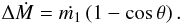 (A.5)Next, we combine Eqs. (16) and (A.5) in order to find the surface density,
 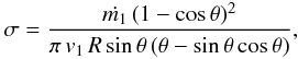 (A.6)where we have used the velocity v given by Eq. (A.4).
In this simple case R = R0/cos θ, and the normal component of the preshock velocity of the stellar wind v1,n = v1 cos θ (see Eq. (6)). Therefore, the pressure  within the thin shell just behind the shock front can be written as
 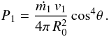 (A.7)Note from Eqs. (7) and (9) that P1 = P2, as expected. From Eq. (15), it follows that the emission measure of the shell is
  . Using Eqs. (A.6) and (A.7), it can be shown that,
 ![Mathematical equation: \appendix \setcounter{section}{1} \begin{eqnarray} EM_{\rm s}= {{ \dot m^2_1 } \over{4\pi^2 \bar{m}^2 c^2_{\rm s} R^3_0}} \left[{{\mbox{cos}^5\theta\,(1 - \mbox{cos}\,\theta)^2} \over{\mbox{sin}\,\theta\,(\theta - \mbox{sin}\,\theta\, \mbox{cos}\,\theta)}}\right]\cdot \label{a8} \end{eqnarray}](/articles/aa/full_html/2011/07/aa15988-10/aa15988-10-eq261.png) (A.8)Let us now calculate the emission measure of the stellar winds. Since we assume the same flow parameters of both components of the binary system, then the emission measure of the winds is given by
(A.8)Let us now calculate the emission measure of the stellar winds. Since we assume the same flow parameters of both components of the binary system, then the emission measure of the winds is given by 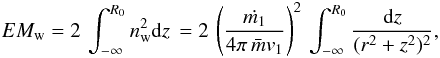 (A.9)and integrating one obtains
 ![Mathematical equation: \appendix \setcounter{section}{1} \begin{eqnarray} EM_{\rm w}= {{\dot m^2_1}\over{16 \pi^2\,\bar{m}^2 v^2_1 r^3}} \left [{{\pi}\over{2}} + {{(r/R_0)}\over{1 + (r/R_0)^2}} + \mbox{arctg}\left({{R_0}\over{r}}\right) \right]\cdot \label{a10} \end{eqnarray}](/articles/aa/full_html/2011/07/aa15988-10/aa15988-10-eq263.png) (A.10)Thus, the total emission measure is given by EM = EMs + EMw.
(A.10)Thus, the total emission measure is given by EM = EMs + EMw.
A.1. The emission measure EM as function of the stagnation point radius R0
Let us now fix the impact parameter r, and investigate the behavior of the emission measure EM as function of the stagnation point radius R0. The total emission measure along a given line of sight can be written as 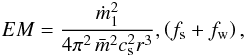 (A.11)where
 ![Mathematical equation: \appendix \setcounter{section}{1} \begin{eqnarray} f_{\rm s}= \left ({{r}\over{R_0}}\right)^3 \, \left[{{\mbox{cos}^5\theta\,(1 - \mbox{cos}\,\theta)^2} \over{\mbox{sin}\,\theta\,(\theta - \mbox{sin}\,\theta\, \mbox{cos}\,\theta)}}\right], \label{a12} \end{eqnarray}](/articles/aa/full_html/2011/07/aa15988-10/aa15988-10-eq269.png) (A.12)and
(A.12)and ![Mathematical equation: \appendix \setcounter{section}{1} \begin{eqnarray} f_{\rm w}= {{1}\over{4}}\, \left ({{c_{\rm s}}\over{v_1}}\right)^2 \, \left [{{\pi}\over{2}} + {{r/R_0}\over{1 + (r/R_0)^2}} + \mbox{arctg}\left({{R_0}\over{r}}\right) \right]\cdot \label{a13} \end{eqnarray}](/articles/aa/full_html/2011/07/aa15988-10/aa15988-10-eq270.png) (A.13)It is also possible to give the emission measure EMs (Eq. (A.8)) in terms of r and R0 by substituting the trigonometric functions
(A.13)It is also possible to give the emission measure EMs (Eq. (A.8)) in terms of r and R0 by substituting the trigonometric functions 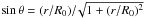 ,
, 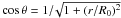 , and θ = arctg(r/R0) into Eq. (A.12).
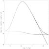 |
Fig. A.1 Nondimension emission measure as function of r/R0. The dotted and dashed lines represent the functions fs of the shocked layer, and fw of the stellar winds, respectively. The total emission measure fs + fw is also shown (solid line). The physical description of the plot is given in the text. |
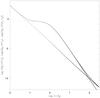 |
Fig. A.2 Nondimension emission measure as function of r/R0. The function (r/R0)-3 fs (dotted line) of the shocked layer, and (r/R0)-3 fw (dashed line) of the stellar winds are presented. The solid line represents the total emission measure (r/R0)-3 (fs + fw). The physical description of the plot is given in the text. |
In Fig. A.1, we present fs and fw as functions of r/R0. We fix the impact parameter r and vary the stagnation point radius R0. We note from the figure that, initially as r/R0 increases (which means closer binary systems), the emission measure from the shell increases. While r/R0 is still growing, the emission measure reaches a maximum value (fs ≃ 1 at r/R0 ≃ 1.3) and then it steadily decreases. In addition, it can be observed from the figure that fs ≫ fw at r/R0 ≃ 1, and fs ≪ fw at very large (r/R0 ≪ 1) or very small (r/R0 ≫ 1) stagnation point radii.
A.2. The emission measure EM as function of the impact parameter r
We now fix the stagnation point radius R0 and investigate the variation of the total emission measure with the impact parameter r. In this case, it is useful to write the total emission measure EM (= EMs + EMw) as  (A.14)In Fig. A.2, we show the contribution of the shell EMs, the contribution of the winds EMw, and the total emission measure EM as functions of the nondimensional impact parameter (r/R0). We note from the figure that the emission measure is dominated by the shell (EMs ≫ EMw) at impact parameters (r/R0) ≃ 1. However, at very low (r/R0 ≪ 1) or very high (r/R0 ≫ 1) values of the impact parameter, the contribution of the stellar winds to the total emission measure is more important (EMs ≪ EMw).
Given the emission measure EMs of the shocked layer, the optical depth τs can be obtained by  (A.15)where
  .
.
For lines of sight with impact parameters r/R0 ≪ 1, it can be shown that fs ≃ 3/8 (r/R0)3, and  (A.16)Consequently, with in this limit the optical depth of the shell τs does not depend on the value of r and scales as D-3 (being D the binary separation).
On the other hand, for higher impact parameters (r/R0 ≫ 1) fs ≃ 2/π (R0/r)2 and  (A.17)Thus, in this limit (τs ∝ r-5), the optical depth of the shell (for a given line of sight) scales as τs ∝ D2.
A.3. Flux density Sν as function of the binary separation D
In this section, we investigate the dependence of the flux density Sν with the binary separation D. Figure A.3 shows the flux density S43 GHz of the shocked layer as function of the nondimensional impact parameter r/R0. We have adopted the wind parameters of Model B2 (see Table 2). It can be seen from the figure that at the beginning the flux grows as r2, which suggests that the emission comes from an optical thick disk. Eventually (at r/R0 ≃ 40), however, the shell becomes optically thin and the flux tends to a constant value. The main contribution to the flux comes from the optically thick region of the shell, and therefore the emission from the optically thin region can be neglected.
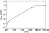 |
Fig. A.3 Integrated flux density at 43 GHz of the shocked layer over the nondimensional impact parameter r/R0. In this example, we have assumed the parameters of the colliding winds of Model B2 (see Table 2). The behavior of the plot is described in the text. |
Let rm be the transition impact parameter at which τs(rm) = 1. Since EMs ≫ EMw for lines of sight with impact parameters r ≤ rm, we assume that the optical depth is dominated by the shell. (For simplicity, we are not considering those impact parameters r ≪ R0 for which EMs ≪ EMw; see Fig. A.1.) It follows that the optical depth 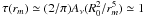 (Eq. (A.16)), and then the size of the optically thick region increases as
  . Finally, since the total flux is dominated by the emission from the optically thick region (r ≤ rm), one can assume that the flux
  . Consequently, we predict from our model that the emission from the shocked layer scales as Sν ∝ D4/5. Detailed calculations (as in the example shown in Fig. A.4), which consider both the contribution of the optically thin region to the emission from the shell and the contribution by the stellar winds to the total optical depth, give a small deviation from this prediction, that is, Sν ∝ D0.79.
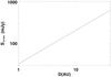 |
Fig. A.4 Predicted flux density at S43 GHz from a binary system as function of the binary separation D. We have adopted the stellar wind parameters of Model B2 (see Table 2). From this example, we found that the flux scales as D0.79. |
All Tables
All Figures
|
Fig. 1 Schematic diagram showing the interaction of two spherical winds that move radially away from the stars. Source 1 of the wind with velocity v1 is located at the origin of the coordinate system, and source 2 of the wind with velocity v2 at a distance D along the symmetry axis. The shape of the layer where the winds collide (at R0 along the symmetry axis) is given by the curve R(θ). The angles θ and θ1 are measured from the positions of the stars to the intersection point between a line of sight (with impact parameter r) and the layer. We assume azimuthal symmetry (no dependence on angle φ). The observer is located in the orbital plane along the z-axis of symmetry. |
| In the text | |
|
Fig. 2 Schematic diagram showing a thin shell (limited by two shock fronts) resulting from the interaction of two stellar winds. The shocked gas flows along the shell at a velocity v and has a surface density σ. The coordinate l is measured inwards from the wind shock of source 2, normal to the locus of the thin shell. |
| In the text | |
|
Fig. 3 Predicted free-free emission from a colliding wind binary. We have adopted the parameters v1 = 103 km s-1, ṁ1 = 1.25 × 10⁻⁵ M⊙ yr-1, and v2 = 103 km s-1, ṁ2 = 5 × 10⁻⁵ M⊙ yr-1 for the wind sources. The binary separation is set to D = 4 AU. The dotted and dashed lines represent the fluxes (∝ ν0.6) from the wind sources 1 and 2 (see also Fig. 1), respectively. The intrinsic thermal emission from the WCR (dot-dashed line) and the total emission (solid line) from the binary system are also shown. The behavior of the curves is described in the main text. |
| In the text | |
|
Fig. 4 Optical depth τWCR(43 GHz) of the WCR as a function of impact parameter r (left panels), and the predicted flux density Sν at radio frequencies (right panels) for the models of Table 1. In top panels, the dot-dashed, solid and dotted lines represent the optical depth and the radio spectrum from the models B1, B2, and B3, respectively. In bottom panels, the corresponding values of models B2, B4, and B5 are shown by the solid, dot-dashed, and dotted lines, respectively. The physical description of the plots are given in the text. |
| In the text | |
|
Fig. 5 Comparison between our model and the flux densities at 5, 8.4, 23 and 250 GHz (“+” sign; uncertainty in the flux measurements are given by the length of the bars) of the binary system WR 98 obtained by Montes et al. (2009) and Altenhoff et al. (1991), respectively. We have assumed the stellar wind parameters ṀWR = 3.0 × 10⁻⁵ M⊙ yr-1, vWR = 1200 km s-1, ṀO = 4.0 × 10⁻⁶ M⊙ yr-1, and vO = 1800 km s-1. The stars are separated by a distance D ~ 0.5 AU. The dotted and dashed lines represent the fluxes (∝ ν0.6) from the winds of the WR and O type stars, respectively. The radiation from the WCR (dot-dashed line) and the total flux density (solid line) from the binary source are also shown. The physical description of the plot is given in the text. |
| In the text | |
|
Fig. 6 Comparison between our model and the flux densities at 5, 8.4, 23 GHz (“+” sign; uncertainty in the flux measurements are given by the length of the bars) of the binary system WR 113 obtained by Montes et al. (2009). We have assumed the stellar wind parameters ṀWR = 2.0 × 10⁻⁵ M⊙ yr-1, vWR = 1700 km s-1, ṀO = 0.4 × 10⁻⁵ M⊙ yr-1, and vO = 1800 km s-1. The stars are separated by a distance D ~ 0.6 AU. The dotted and dashed lines represent the fluxes (∝ ν0.6) from the winds of the WR and O type stars, respectively. The radiation from the WCR (dot-dashed line) and the total flux density (solid line) from the binary source are also shown. The physical description of the plot is given in the text. |
| In the text | |
|
Fig. A.1 Nondimension emission measure as function of r/R0. The dotted and dashed lines represent the functions fs of the shocked layer, and fw of the stellar winds, respectively. The total emission measure fs + fw is also shown (solid line). The physical description of the plot is given in the text. |
| In the text | |
|
Fig. A.2 Nondimension emission measure as function of r/R0. The function (r/R0)-3 fs (dotted line) of the shocked layer, and (r/R0)-3 fw (dashed line) of the stellar winds are presented. The solid line represents the total emission measure (r/R0)-3 (fs + fw). The physical description of the plot is given in the text. |
| In the text | |
|
Fig. A.3 Integrated flux density at 43 GHz of the shocked layer over the nondimensional impact parameter r/R0. In this example, we have assumed the parameters of the colliding winds of Model B2 (see Table 2). The behavior of the plot is described in the text. |
| In the text | |
|
Fig. A.4 Predicted flux density at S43 GHz from a binary system as function of the binary separation D. We have adopted the stellar wind parameters of Model B2 (see Table 2). From this example, we found that the flux scales as D0.79. |
| In the text | |
Current usage metrics show cumulative count of Article Views (full-text article views including HTML views, PDF and ePub downloads, according to the available data) and Abstracts Views on Vision4Press platform.
Data correspond to usage on the plateform after 2015. The current usage metrics is available 48-96 hours after online publication and is updated daily on week days.
Initial download of the metrics may take a while.