| Issue |
A&A
Volume 530, June 2011
|
|
|---|---|---|
| Article Number | A69 | |
| Number of page(s) | 14 | |
| Section | Planets and planetary systems | |
| DOI | https://doi.org/10.1051/0004-6361/201116449 | |
| Published online | 11 May 2011 | |
Flux and polarisation spectra of water clouds on exoplanets
1
SRON – Netherlands Institute for Space Research, Sorbonnelaan 2, 3584 CA Utrecht, The Netherlands
e-mail This email address is being protected from spambots. You need JavaScript enabled to view it.
2
Astronomical Institute “Anton Pannekoek”, University of Amsterdam, Science Park 904, 1098 XH Amsterdam, The Netherlands
3
Astronomical Institute, Utrecht University, Princetonplein 5, 3584 CC Utrecht, The Netherlands
Received: 6 January 2011
Accepted: 7 April 2011
Abstract
Context. A crucial factor for a planet’s habitability is its climate. Clouds play an important role in planetary climates. Detecting and characterising clouds on an exoplanet is therefore crucial when addressing this planet’s habitability.
Aims. We present calculated flux and polarisation spectra of starlight that is reflected by planets covered by liquid water clouds with different optical thicknesses, altitudes, and particle sizes, as functions of the phase angle α. We discuss the retrieval of these cloud properties from observed flux and polarisation spectra.
Methods. Our model planets have black surfaces and atmospheres with Earth-like temperature and pressure profiles. We calculate the spectra from 0.3 to 1.0 μm, using an adding-doubling radiative transfer code with integration over the planetary disk. The cloud particles’ scattering properties are calculated using a Mie-algorithm.
Results. Both flux and polarisation spectra are sensitive to the cloud optical thickness, altitude and particle sizes, depending on the wavelength and phase angle α.
Conclusions. Reflected fluxes are sensitive to cloud optical thicknesses up to ~40, and the polarisation to thicknesses up to ~20. The shapes of polarisation features as functions of α are relatively independent of the cloud optical thickness. Instead, they depend strongly on the cloud particles’ size and shape, and can thus be used for particle characterisation. In particular, a rainbow strongly indicates the presence of liquid water droplets. Single scattering features such as rainbows, which can be observed in polarisation, are virtually unobservable in reflected fluxes, and fluxes are thus less useful for cloud particle characterisation. Fluxes are sensitive to cloud top altitudes mostly for α < 60° and wavelengths <0.4 μm, and the polarisation for α around 90° and wavelengths between 0.4 and 0.6 μm.
Key words: polarization / methods: numerical / radiative transfer / planets and satellites: atmospheres / Earth
© ESO, 2011
1. Introduction
Since the discovery of the first exoplanet orbiting a solar–type star more than a decade ago (Mayor & Queloz 1995), the quest for signs of habitable exoplanets has started. And while many scientists intertwine habitability with the existence of liquid water on the planetary surface, another key factor for habitability is the planetary climate (Kasting et al. 1993). Clouds are among the major factors that affect a planetary climate.
Regarding the Earth, Goloub et al. (2000) presented an extended series of studies of the Earth’s climate both at an observational as well as at a modelling level, which clearly indicates the crucial and diverse roles of clouds. In particular, clouds are responsible for the modulation of both the shortwave radiation (from the sun) as well as the long-wave radiation (from the planet) budgets of the Earth (Kim & Ramanathan 2008; Ramanathan et al. 1989; Cess et al. 1992; Malek 2007; and others). Additionally, by modulating the solar radiation clouds affect the atmospheric photolysis rates, which change the atmospheric photochemistry and chemical composition (Pour Biazar et al. 2007). And clouds are responsible for the storage of atmospheric volatiles, such as the organic volatiles that are indicators of the existence of bio and fossil–masses, which can damage the soil and groundwater and can react with sunlight to create tropospheric O3 (Klouda et al. 1996). Because of their roles in the climate, clouds on Earth have been subjected to intense study for the past five decades, both from a theoretical/modelling point of view, as well as from an observational point of view (from the ground as well as from space). The effects of clouds on the Earth’s climate have been shown to depend on the sizes and shapes (i.e. thermodynamical phase) of the cloud particles, and on the optical thickness and vertical extension of a cloud.
In this paper, we present results of numerical simulations of flux and especially polarisation spectra of starlight that is reflected by cloudy exoplanets, and discuss the sensitivity of these spectra to the size of the cloud particles, the cloud optical thickness and the cloud top altitude. In general, the composition of a cloud or cloud layer in a planetary atmosphere will depend on the ambient chemical composition, and the pressure and temperature profiles (the latter themselves will of course also be influenced by the presence of clouds). It is well known that clouds have strong effects on flux spectra of planets in the Solar System and beyond. Examples of simulated flux spectra of exoplanets with water clouds can be found in Marley et al. (1999); Tinetti et al. (2006); Kaltenegger et al. (2007). Far less work has been done regarding polarisation spectra of cloudy planets. Examples of simulated polarisation spectra of exoplanets with liquid water clouds can be found in Stam (2008). In this paper we extend this work to different types of clouds, at various altitudes.
Terrestrial liquid water clouds are in general comprised of particles with radii ranging from ~5 μm to ~30 μm (Han et al. 1994), and their optical thickness varies typically from b ~ 1 to b ~ 40 or more (van Deelen et al. 2008). There appears to be a correlation between the cloud particle sizes and the cloud optical thickness (Han et al. 1994, and references therein), that could originate in the properties of the condensation nuclei that the cloud partices condense on, but it is not a strong one (Stephens et al. 2008). Knowing the sizes of cloud particles is important for understanding a cloud’s influence on a planetary climate, because it determines how a cloud particle scatters and absorbs incident light and thermal radiation (see e.g. Chapman et al. 2009, and references therein). How a particle scatters the light depends in particular on the size parameter, i.e. the ratio of 2π times the particle radius to the wavelength (see Eq. (9)). We will consider size parameters ranging from less than 1 up to ~120, covering the so-called Rayleigh regime, where the scattering particles are much smaller than the wavelength, to the geometric optics regime, where particles are large with respect to the wavelength. The cloud’s optical thickness (which, when assuming spherical particles, is the product of the column number density and the extinction cross-section of the cloud particles) depends on the cloud particles’ sizes, shapes, and composition, and hence also on the wavelength of the radiation. We will use cloud optical thicknesses ranging from 0.5 to 60 (at 0.55 μm) and spherical water particles.
Another cloud parameter that is not only important for the radiation field, but also for the thermo- and hydro-dynamical processes that take place in planetary atmospheres is the altitude or pressure of the top of the cloud. Cloud top altitudes and pressures are routinely determined in Earth remote-sensing and regularly in planetary observations (e.g. Wark & Mercer 1965; Weigelt et al. 2009; Peralta et al. 2007; Garay et al. 2008; Matcheva et al. 2005). In Earth and planetary observations, knowledge of cloud top altitudes is also essential for accurate derivations of mixing ratios of atmospheric trace gases from the depths of gaseous absorption bands in planetary spectra, since clouds will change the band depths. For example, in Earth observation, cloud top altitudes are used in the retrieval of the trace gas ozone (O3). These cloud top altitudes are usually derived from the depth of the so-called A absorption band of the well–mixed gas oxygen (the O2 A band is located around 0.76 μm) (e.g. Yamamoto & Wark 1961 and Fischer & Grassl 1991). Note that in case an absorbing gas is not well-mixed and its vertical distribution is not known, its absorption bands cannot be used to provide absolute cloud tops.
Clouds on Earth are found at a wide range of altitudes. Most clouds are located in the troposphere, the lowest portion of the atmosphere, where the temperature generally decreases with altitude. On average, the top of the troposphere decreases with increasing latitude, and with that the maximum cloud top altitude, from about 20 km in the tropics, to about 10 km in the polar regions. The tops of the highest clouds will usually contain ice particles. The thin, whisphy clouds commonly known as cirrus clouds, are composed entirely of water ice crystals. Since above the tropopause, the atmosphere contains relatively little water vapour, most types of clouds are confined to the troposphere. The few cloud types that can be found above the tropopause are thin ice clouds, such as polar stratospheric clouds and noctilucent clouds.
We will limit ourselves to clouds that are composed entirely of liquid water droplets, and hence limit the cloud top altitudes in our model atmospheres to about 4 km (where the temperatures are still high enough to exclude the presence of ice particles). Our main reason to exclude clouds with ice particles is that the single scattering properties of ice (crystal) particles are usually very different from those of liquid (spherical) particles (see e.g. Goloub et al. 2000), and as a result, their presence will influence the light that is reflected by a cloud (in particular the polarised signal). Modelling and analysing this influence (which will depend on absolute and relative ice particle number densities, ice particle sizes and shapes, and orientation) will be the subject of further research.
In this paper, we present not only numerically simulated flux spectra, but especially polarisation spectra. Polarimetry, i.e. measuring the direction and degree of polarisation of light, is considered to be a powerful tool for the direct detection of exoplanets (Keller 2006; Keller et al. 2010; Stam et al. 2004). The reason for this is that, when integrated over the stellar disk, starlight of solar type stars will be virtually unpolarised (Kemp et al. 1987), while starlight that has been reflected by an exoplanet will generally be polarised, due to scattering and reflection processes in the planetary atmosphere and on the surface (if present). Polarimetry can thus enhance the contrast between a planet and its star by a factor of ~104 − ~ 105 (Keller et al. 2010), and thus facilitate the direct detection of an exoplanet. Another advantage of polarimetry for exoplanet detection is that it enables the direct confirmation of a detection, since the degree and direction of polarisation of a detected object will exclude it being a background star.
The real strength of polarimetry for exoplanet research is, however, that it cannot only be used for the direct detection of exoplanets, but also for the characterisation of the physical properties of these planets. The reason is that the state of polarisation of starlight that is reflected by a planet is very sensitive to the composition and structure of the planetary atmosphere and surface (if present) (see Hansen & Travis 1974; Hovenier et al. 2004; Mishchenko et al. 2010, and references therein). An early example of this application of polarimetry is the derivation of the composition and size distribution of the droplets forming the upper Venusian clouds as well as the cloud top altitudes from Earth-based, disk-integrated Venus observations by Hansen & Hovenier (1974).
The application of polarisation for the detection and characterisation of exoplanets has been shown for gaseous exoplanets by e.g. Seager et al. (2000); Saar & Seager (2003); Stam (2003); Stam et al. (2004) and for terrestrial planets by Stam (2008). Note that in the first two papers, planets are considered that are too close to their star to be spatially resolved. The observable degree of polarisation for these systems is thus the ratio of the polarised flux of the planet to the total flux of the star (plus that of the planet), and consequently, very small. In the latter three papers, the planet is assumed to be spatially resolvable from its star. In that case, the observable degree of polarisation is thus the degree of polarisation of the planet itself (apart from a contribution of unpolarized background starlight), which can be several tens of percents. In this paper, we will consider spatially resolvable planets. Our results can straightforwardly be applied to spatially unresolvable planets by scaling them with the stellar flux.
The simulations we present in this paper are useful for the design, development, and optimisation of instruments for the direct detection of exoplanets. Since the presence of water-clouds is not restricted to terrestrial planets, these can be instruments for the detection of gaseous planets and/or terrestrial planets, and both for ground- and space-based telescopes. An example of such an instrument is SPHERE (Spectro-Polarimetric High-contrast Exoplanet Research), a second generation planetfinder instrument for the European Southern Observatory’s (ESO) Very Large Telescope (VLT). For SPHERE, first light is expected in 2012. SPHERE has broadband polarimetric capabilities in the I-band (0.6 − 0.9 μm). EPICS (ExoPlanets Imaging Camera and Spectrograph) has been proposed as the planetfinder instrument for ESO’s Extremely Large Telescope (ELT), and will also have a polarimeter to detect and characterise exoplanets. EPICS is still in its design and optimisation phase, and first light is expected not earlier than 2020. An example of a space telescope concept for exoplanet research that would be ideally suited to observe both the flux and the state of polarisation of starlight that is reflected by exoplanets is the New Worlds Observer (NWO) that has been and will be proposed to NASA (Oakley & Cash 2009; Cash & New Worlds Study Team 2010). An example of a space-telescope with polarimetric capabilities for exoplanet research that has been proposed to the European Space Agency in response to its Cosmic Vision 2015 − 2020 call for a medium sized mission (M3), is Spectro-Polarimetric Imaging and Characterization of Exo-planetary Systems, or SPICES.
This paper is organised as follows. In Sect. 2, we give a general description of light, including polarisation, and present the radiative transfer algorithm we use for our numerical simulations of starlight that is reflected by planets. In Sect. 3, we describe our model atmospheres and in Sect. 4 the flux and degree of polarisation of light that has been singly scattered by the model cloud particles. In Sects. 5.1 and 5.2, we show the results of our numerical simulations of the flux and degree of polarisation of reflected starlight for different cloud particle microphysical properties, and in Sect. 5.3, for different cloud top pressures. Finally, in Sects. 6 and 7 we summarise and discuss our results and future work.
2. Description of starlight that is reflected by an exoplanet
Light that has been reflected by an exoplanet can be fully described by a flux vector πF, as follows: ![Mathematical equation: \begin{equation} \label{eq:first} \pi\vec{F} = \pi\left[\begin{array}{c} F \\ Q \\ U \\ V \end{array}\right]\!, \end{equation}](/articles/aa/full_html/2011/06/aa16449-11/aa16449-11-eq20.png) (1)where parameter πF is the total reflected flux, parameters πQ and πU describe the linearly polarised flux and parameter πV the circularly polarised flux (see e.g. Hansen & Travis 1974; Hovenier et al. 2004; Stam 2008). All four parameters are wavelength dependent and their dimensions are W m-2 m-1. Parameters πQ and πU are defined with respect to the so-called planetary scattering plane, i.e. the plane through the centers of the planet, the host star and the observer (see Stam 2008).
(1)where parameter πF is the total reflected flux, parameters πQ and πU describe the linearly polarised flux and parameter πV the circularly polarised flux (see e.g. Hansen & Travis 1974; Hovenier et al. 2004; Stam 2008). All four parameters are wavelength dependent and their dimensions are W m-2 m-1. Parameters πQ and πU are defined with respect to the so-called planetary scattering plane, i.e. the plane through the centers of the planet, the host star and the observer (see Stam 2008).
The degree of polarisation P is defined as the ratio of the polarised flux to the total flux, as follows:  (2)In case a planet is mirror–symmetric with respect to the planetary scattering plane, and for unpolarised incoming stellar light, the disk integrated fluxes πU and πV of the reflected light will equal zero due to symmetry (see Hovenier 1970) and we can use the following, alternative, definition of the degree of polarisation that includes the direction of polarisation
  (3)For Ps > 0 (i.e. Q < 0), the light is polarised perpendicular to the reference plane, while for Ps < 0 (i.e. Q > 0) the light is polarised parallel to the reference plane.
The flux vector πF of stellar light that has been reflected by a spherical planet with radius r at a distance d from the observer (d ≫ r) is given by (Stam et al. 2006)  (4)Here, λ is the wavelength of the light and α the planetary phase angle, i.e. the angle between the star and the observer as seen from the center of the planet. Furthermore, S is the 4 × 4 planetary scattering matrix (Stam et al. 2006) and πF0 is the flux vector of the incident stellar light. For a solar type star, the stellar flux can be considered to be unpolarised when integrated over the stellar disk (Kemp et al. 1987). Further assuming that the stellar light is unidirectional, we can thus describe πF0 as (see Eq. (1))
  (5)with πF0 the flux of the stellar light that is incident on the planet measured perpendicular to the direction of incidence, and 1 the unit column vector.
For unpolarised incident stellar light (see Eq. (5)) and for a planet that is mirror–symmetric with respect to the planetary scattering plane, the degree of polarisation Ps (Eq. (3)) of the light that is reflected by the planet depends on only two elements of the scattering matrix, as follows  (6)(for a derivation see Stam 2008). Since the degree of polarisation is a relative measure, it has no dependence on planetary and stellar radii, distances, nor on the incident stellar flux.
In this paper, we present numerically simulated flux and polarisation spectra of planets that are completely covered by water clouds as functions of the planetary phase angle α. Even though such a model is probably not very realistic, in this first study we will use it in order to limit the number of parameters we need to study in our models, and to get some first idea on the important features we need to investigate in planetary signals. We assume that the ratio of the planetary radius r and the distance to the observer d is equal to one, and that the incident stellar flux πF0 is equal to 1 W m-2 m-1. The hence normalised flux πFn that is reflected by a planet is thus given by  (7)(see Stam 2008), and corresponds to the planet’s geometric albedo AG if α = 0° (AG is defined as the ratio of the total flux πF that is reflected by the planet at α = 0°, to the flux πFL that is reflected by a Lambertian surface subtending the same solid angle on the sky). Our normalised fluxes πFn can straightforwardly be scaled for any given planetary system using Eq. (4) and inserting the appropriate values for r, d and πF0. As mentioned above, the degree of polarisation Ps is independent of r, d and πF0, and will thus not require any scaling.
To calculate the planetary scattering matrix elements a1 and b1 of the reflected stellar light, we employ the algorithm described in Stam et al. (2004), which consists of an efficient and accurate adding-doubling algorithm (de Haan et al. 1987) in combination with a fast, numerical, disk integration algorithm, to calculate the radiative transfer in the locally plane-parallel planetary atmosphere, and to integrate the reflected light across the illuminated and visible part of the planetary disk.
3. Our model atmospheres
The model planetary atmospheres we use in our numerical simulations are composed of stacks of horizontally homogeneous and locally plane-parallel layers, which contain gas molecules and, optionally, cloud particles. We create vertically inhomogeneous atmospheres simply by stacking different, homogeneous layers. Each atmosphere is bounded below by a flat, homogeneous surface. We base our atmospheric temperature and pressure profiles on representative ones of the Earth’s atmosphere (McClatchey et al. 1972). Here, we use only four atmospheric layers (see Table 1 for the pressures and temperatures at the tops of these layers) and a black planetary surface. The molecular or Rayleigh scattering optical thickness, of each atmospheric layer and its spectral variation is calculated as described in Stam (2008) assuming an atmospheric gas composition of the model atmospheres that is similar to that of the Earth. For our simulations of the flux and polarisation spectra, we focus on the continuum, and we ignore absorption by atmospheric gases (such as O2, H2O and O3). Even though we use pressure and temperature profiles and a gas composition that are typical for an Earth-like planet, most of our results are also applicable to other planets, e.g. gas giants with high altitude water clouds.
The altitude (in km), pressure (in bar), and temperature (in K) at the bottom and top of each layer of our model atmosphere (McClatchey et al. 1972).
We will use a clear model atmosphere, i.e. without clouds, and cloudy model atmospheres. In the latter, one of the atmospheric layers contains cloud particles in addition to the gas molecules. To study the dependence of the flux and degree of polarisation of the starlight that is reflected by the model planet on the altitude of the top of the cloud layer, we will use the following three cases: a low cloud layer, with its top at an ambient pressure of 0.802 bar (corresponding to an altitude of 2 km on Earth), a middle cloud layer, with its top at 0.710 bar (3 km on Earth), and a high cloud layer, with its top at 0.628 bar (4 km on Earth). Unless stated otherwise the geometrical thickness of the cloud layer is 1 km.
Optical thicknesses of clouds on Earth show a huge variation on daily and monthly timescales and from place to place. In particular, the optical thickness in completely cloudy cases can reach values up to 40 (van Deelen et al. 2008) or more. The optical thickness b of our cloud layers is chosen to range between 0.5 and 60 (at λ = 0.55 μm). Our standard cloud layer has an optical thickness of 10 (at λ = 0.55 μm), which appears to be an average value. The spectral variation of the cloud layer’s optical thickness depends on the microphysical properties of the cloud particles, such as their composition, shape and size (see below).
Our model cloud layers are composed of liquid, spherical water particles. Water cloud observations on Earth show a large variation in droplet sizes that is attributed to, amongst others, a variation in the number density and composition of cloud condensation nuclei (Han et al. 1994; Martin et al. 1994; Segal & Khain 2006). In particular, typical cloud particle radii range from about 5 μm to 15 μm, with a global mean value of about 8.5 μm above continental areas, and 11.8 μm above maritime areas (Han et al. 1994). On the lower limit, sizes down to 2 μm have been reported from satellite measurements (Minnis et al. 1992), and on the upper limit, sizes up to 25 μm (Goloub et al. 2000).
We describe the sizes of our cloud particles by a standard size distribution (Hansen & Travis 1974), as follows  (8)where C is a normalisation constant, n(r)dr is the number of particles with radii between r and r + dr per unit volume, and reff and veff are the effective radius and variance, respectively (see Hansen & Travis 1974). The units of reff are [μm], while veff is dimensionless.
The scattering properties of particles often depend strongly on the ratio of the radius of the particles to the wavelength of the light. This so-called effective size parameter, xeff, that will be used later in this paper, is defined as  (9)(see Hansen & Travis 1974). For xeff ≪ 1, the scattering is usually referred to as Rayleigh scattering, and for xeff ≫ 1, we get into the regime where light scattering can be described with geometrical optics.
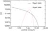 |
Fig. 1 Particle size distributions (see Eq. (8)) for model A particles (reff = 2.0 μm, veff = 0.1; red, dashed line) and model B particles (reff = 6.0 μm, veff = 0.4; black, solid line). Each size distribution has been normalised such that the integral over all sizes equals 1. |
Our cloud layers are composed of either small model A particles with reff = 2.0 μm and veff = 0.1 (Stam 2008), or larger model B particles with reff = 6.0 μm and veff = 0.4. The latter are similar to those used by van Diedenhoven et al. (2007), who consider this to represent an average terrestrial water cloud. Figure 1 shows the size distributions of the particles of the two standard models used further in this paper (A and B particles). To study the influence of a size distribution’s effective variance veff on the reflected light, we will also use model A2 particles with reff = 2.0 μm and veff = 0.4, and model B2 particles with reff = 6.0 μm and veff = 0.1 (see Table 2).
The effective radius reff (in μm) and variance veff of the standard size distributions (see Hansen & Travis 1974, and Eq. (15)) that describe our model cloud particles.
The real part of the refractive index of water in the wavelength region of our interest is slightly wavelength dependent. It varies from 1.344 at λ = 0.4 μm, to 1.320 at 1.0 μm (Daimon & Masumura 2007; van Diedenhoven et al. 2007). The imaginary part of the refractive index is small but varies strongly (Pope & Fry 1997), from about 10-8 at 0.3 μm, to about 10-5 at 1.0 μm, with a minimum of 8 × 10⁻¹⁰ at 0.5 μm. We use a constant refractive index that is equal to 1.335 ± 0.00001i. We checked that our results are virtually insensitive to the assumption of a constant value of the refractive index.
Given the wavelength, refractive index, effective radius reff and variance veff, we calculate the cloud particles’ extinction cross-section, single scattering albedo, and the expansion coefficients of the single scattering matrix in generalised spherical functions (see Hovenier et al. 2004) using Mie theory (van de Hulst 1957; de Rooij & van der Stap 1984). With the hence obtained extinction cross-sections, we calculate the cloud layer’s optical thickness at wavelengths other than 0.55 μm. Figure 2 shows the spectral variation of the absorption and scattering optical thicknesses of four cloud layers, each with a total optical thickness of 2.0 at λ = 0.55 μm, that are composed of the model A, A2, B and B2 particles, respectively. As can be seen in the figure, the effective variance veff plays only a minor role in determining the cloud’s scattering and absorption optical thicknesses.
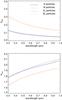 |
Fig. 2 Spectral variation of the absorption (upper panel) and scattering (lower panel) optical thicknesses, babs and bsca, of cloud layers composed of the following model particles (see Table 2): A (reff = 2.0 μm, veff = 0.1; black, solid line), A2 (reff = 2.0 μm, veff = 0.4; blue, dashed–dotted line), B (reff = 6.0 μm, veff = 0.4; red, dashed line), and B2 (reff = 6.0 μm, veff = 0.1; orange, dashed–tripple–dotted line). The total optical thickness (b = bsca + babs) of each cloud layer is 2.0 at λ = 0.55 μm. |
4. Single scattering properties of water cloud particles
The degree of polarisation of the starlight that is reflected by a planet is very sensitive to the single scattering properties of the atmospheric particles (see e.g. Hansen & Travis 1974). The reason for this is that due to the generally low degree of polarisation of multiple-scattered light, the main angular features observed in a polarised planetary signal will be due to single scattered light. The contribution of the multiple scattered light to the signal is mostly to decrease the overall degree of polarisation, not to change the shape or angular distribution of the features. Thus, in order to understand the features observed in starlight that is reflected by a planet, as presented in Sect. 5, knowledge of the single scattered light is essential.
In this section, we therefore present and discuss the flux and degree of polarisation of incident unpolarized light Ps that is singly scattered by our model liquid water cloud particles as functions of the single scattering angle Θ and the wavelength λ. The flux as a function of Θ is usually referred to as the (flux) phase function, and we will refer to Ps as a function of Θ as the polarised phase function.
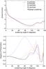 |
Fig. 3 Phase function on a logarithmic scale (upper panel) and degree of polarisation Ps (lower panel) for incident unpolarised light at λ = 0.55 μm that is singly scattered by our model water cloud particles (see Table 2) as functions of the scattering angle Θ: model A (black, solid lines), model B (red, dashed lines), model A2 (blue, dashed-dotted lines) and model B2 (orange, dashed-triple-dotted lines). For comparison, the phase function and Ps are also shown for gas molecules (i.e. Rayleigh scattering) (purple, long-dashed lines). |
Figure 3 shows the flux and Ps of the four model cloud particles A, B, A2 and B2 (see Table 2 for their sizes) as functions of the scattering angle Θ at λ = 0.55 μm. For comparison, we have also added the phase function of the gas molecules (Rayleigh scattering) using an Earth-like depolarization factor, i.e. 0.028 (Bates 1984). The flux phase functions are normalised such that their average over all scattering directions equals unity; they thus do not include the particles’ single scattering albedo.
As can be seen in Fig. 3, Ps of light that is singly scattered by the gas molecules and by the model cloud particles equals zero at Θ = 0° (forward scattering) and 180° (backward scattering). The reason for this is that the incoming light is unpolarised and that at these scattering angles, the scattering process is symmetric with respect to the incoming and the scattered light. The phase function and Ps of Rayleigh scattered light is smooth and symmetric around Θ = 90°. The maximum value of Ps of this light is 0.94 (i.e. 94%).
The flux phase functions of all four types of cloud particles have a strong peak in the forward scattering direction due to light that is diffracted by the particles and the so-called glory in the backscattering direction (cf. Hansen & Travis 1974). The polarisation phase functions of the cloud particles have several interesting features. In particular, for each particle type, Ps changes sign (thus direction), several times between Θ = 0° and 180°. For Θ ≲ 50°, the angular features of Ps appear to be insensitive to the particle size, while for larger scattering angles, the features depend clearly on reff and veff.
Between Θ = 135° and 150°, the phase functions of all four types of cloud particles show a local maximum that is usually referred to as the (primary) rainbow, which is formed by light that has been reflected once inside the particles (see van de Hulst 1957; Hansen & Travis 1974). These rainbows are clear indicators of the spherical shape of the scattering particles, and their angular position depends strongly on the composition (refractive index) of the scattering particles (see Hansen & Travis 1974) and slightly on reff of the particles (see below). While especially for the small cloud particles (models A and A2), the primary rainbow is hardly visible in the flux phase function (see Fig. 3), in Ps it is the strongest and most prominent angular feature for each of the four cloud particle types. Note that the rainbows that are seen in the Earth’s sky during showers are not formed in cloud particles, but in raindrops. On Earth, raindrops have radii on the order of millimeters, corresponding to xeff ≫ 1000 at visible wavelengths.
For reff = 2 μm (particles A and A2), the rainbow is located at Θ ≈ 148°. For reff = 6 μm (particles B and B2), the rainbow is more pronounced and shifted to slightly smaller scattering angles, i.e. to Θ ≈ 143°. The strength of the primary rainbow in Ps depends on reff and on veff; the smaller reff, the smaller the maximum value of Ps in the primary rainbow, and the smaller veff, the larger this maximum value. In particular, for reff = 2.0 μm and veff = 0.1 (model A), Ps of the primary rainbow is 0.58 (58%), while for reff = 2.0 μm and veff = 0.4 (A2), it is 0.50. For reff = 6.0 μm and veff = 0.1 (B), Ps of the primary rainbow is 0.80, and for reff = 6.0 μm and veff = 0.4 (B2), Ps = 0.69. The scattering angle of the primary rainbow (Θ where Ps is maximum) depends mostly on reff: at λ = 0.55 μm, the angle is 150° for reff = 2.0 μm (A and A2) and 143° for reff = 6.0 μm (B and B2).
For the large particles, a secondary peak in the flux phase function is visible around Θ ≈ 120°. This peak is the secondary rainbow, which is formed by light that has been reflected twice inside the particles. While in the phase function this rainbow is hardly visible, and only for the largest particles, Ps clearly shows the secondary rainbow for all four cloud particle types: for reff = 6.0 μm (B and B2) around Θ = 120°, and for the smaller particles at slightly smaller angles. Noteworthy is the minor peak around 155° in Ps of the large B2 particles; this is a supernumerary arc (see e.g. Dave 1969). For the same particles we see a peak around Θ ~ 100°, which could also be a supernumerary arc. Supernumerary arcs are interference features, which explains their washing out with increasing veff.
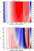 |
Fig. 4 Phase function on a logarithmic scale (upper panel) and degree of polarisation Ps (lower panel) for incident unpolarised, singly scattered light as functions of the scattering angle Θ and the effective size parameter xeff = 2πreff/λ for model cloud particles with veff = 0.1, i.e. models A and B2. For model A (with reff = 2.0 μm), the curves shown in Fig. 3 correspond to xeff = 23, while for model B2 (with reff = 6.0 μm), they correspond to xeff = 69. |
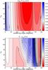 |
Fig. 5 Similar to Fig. 4, except for particles with veff = 0.4, i.e. models A2 and B. For model A2 (with reff = 2.0 μm), the curves shown in Fig. 3 correspond to xeff = 23, while for model B (with reff = 6.0 μm), they correspond to xeff = 69. |
The effects of reff and veff on the singly scattered light are even more clear from Figs. 4 and 5, which show the scattered flux and Ps as functions of Θ and the effective size parameter xeff (cf. Eq. (9)) for veff = 0.1 (A and B2) and veff = 0.4 (A2 and B), respectively. Similar graphs for other size distributions and refractive indices can be found in, for example, Hansen & Travis (1974) and Hansen & Hovenier (1974). The curves shown in Fig. 3 correspond to horizontal cuts in Figs. 4 and 5, at xeff = 23 (reff = 2 μm and λ = 0.55 μm; particles A and A2) and xeff = 69 (reff = 6 μm and λ = 0.55 μm; particles B and B2), respectively.
Comparing the graphs of the flux phase functions in Figs. 4 and 5, it is clear that the phase function depends mostly on xeff, thus on the ratio 2πreff/λ, and that it is not very sensitive to veff, which mostly determines the smoothness of the phase function, i.e. the larger veff, the more subdued the angular variation in the phase function (for a given reff) (see Hansen & Travis 1974). Additionally, we see that Ps appears to be somewhat more sensitive to veff than the flux phase function, but the overall appearance of Ps is the same for the two values of veff. In particular, for Θ < 20°, both figures show a peninsula with small values of Ps. As can also be seen in Hansen & Travis (1974) and Hansen & Hovenier (1974) the shape of this peninsula is sensitive to veff for small values of xeff.
In both Figs. 4 and 5, the primary rainbow (just below Θ = 150°) is only a slight crest in the flux phase functions, but by far the strongest feature in the polarisation phase functions. The strength of the polarised primary rainbow increases with increasing xeff. In other words, for particles with a given reff, the strength of the rainbow increases towards the blue, and/or at a given wavelength, the strength of the rainbow increases with increasing reff. Interesting to note is that for small values of xeff (i.e. ≤ 60), the primary rainbow shifts to larger values of Θ with decreasing xeff, i.e. for a given effective particle radius reff, the rainbow shifts to larger values of Θ towards the red. Consequently, when observed with polarimetry, the rainbow in visible light that is scattered by small water cloud particles should be inverted in colour, compared to the rainbow of light that is scattered by water raindrops (this can not be observed in the flux since the rainbow is virtually unobservable in the flux of light scattered by small cloud particles).
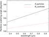 |
Fig. 6 Scattering angle Θ where the primary rainbow in Ps occurs as a function of the wavelength for the model A (reff = 2.0 μm) and B2 (reff = 6.0 μm) particles. |
This colour inversion is shown more clearly in Fig. 6, where the scattering angle of the primary rainbow in Ps is plotted as a function of λ for the model A and B2 particles. For the smallest particles, the rainbow angle increases from 147° at λ = 0.3 μm, to 157° at λ = 1.0 μm. From these and other numerical simulations (not shown) it appears that dΘ/dλ decreases with increasing reff until reff ≈ 20 μm. Indeed, for particles with xeff ~ 100 whitish rainbows (so-called fogbows), are observed in flux (Adam 2002). For much larger particles, such as rain drops, dΘ/dλ becomes negative and decreases further with increasing reff. We checked that the behavior of dΘ/dλ that we calculated is not affected by our choice of using a wavelength independent refractive index, nor by our choice of the particle size distribution.
Our single scattering results suggest that in particular observing the dispersion of the primary rainbow in polarisation would be a useful tool in the retrieval of cloud particle shapes and sizes in exoplanetary atmospheres. To evaluate the usefulness of this tool, numerical simulations of multiple scattered light are required. Results of such simulations are presented and discussed in Sect. 5.
5. Light that is reflected by planets
In the previous section we have presented the single scattering phase functions of our model cloud particles. Here, we present the normalised flux πFn and the degree of polarisation Ps of (single and multiple scattered) starlight that is reflected by a planet as a whole, thus integrated over the illuminated and visible part of the planetary disk. We show the dependence of πFn and Ps on the cloud optical thickness in Sect. 5.1, on the size of the cloud particles in Sect. 5.2, and on the cloud top pressure in Sect. 5.3. We show πFn and Pn as functions of the planetary phase angle α, which equals 180°−Θ, with Θ the single scattering angle.
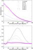 |
Fig. 7 Normalised flux πFn (upper panel) and Ps (lower panel) at λ = 0.55 μm, as functions of the planetary phase angle α for model planets with a cloudfree atmosphere (black solid line) and with atmospheres containing a cloud layer ranging from 3 to 4 km, composed of model A cloud particles, with the following cloud optical thicknesses b (at λ = 0.55 μm): 0.5 (red, dashed lines), 1.0 (green, dash-dotted lines), 10.0 (blue, dash-triple-dotted lines), 20.0 (orange, long-dashed lines), 40.0 (pink, diamond lines), and 60.0 (purple, cross lines). |
5.1. The effects of the cloud optical thickness
Figure 7 shows πFn and Ps of light reflected by cloudy planets as functions of the phase angle α. At α = 0°, the planet’s illuminated side is fully visible, and at α = 180°, we see the planet’s night side. The cloud layer on each planet is composed of model A particles (see Table 2), and the cloud top pressure is 0.628 bar (on Earth this would correspond to a cloud top altitude of 4 km, see Table 1). At 0.55 μm, the molecular scattering optical thickness of the whole model atmosphere is 0.098, and that of the gaseous atmosphere above the cloud 0.06. In the figure, the cloud optical thickness varies from 0 (i.e. no cloud at all) to 60 (at λ = 0.55 μm). Note that a cloud optical thickness of 60 appears to be very large for a 1 km thick cloud. We have included this large value in our simulations for the purpose of comparison.
As can be seen in Fig. 7, the quasi-monochromatic geometric albedo AG the cloudfree planet is as small as 0.063, which is due to the black surface and the small atmospheric (molecular) scattering optical thickness. The normalised flux πFn decreases smoothly with α. The degree of polarisation Ps of the cloudfree planet is zero at α = 0° (due to symmetry) and 180° (due to first order scattering, see Hovenier & Stam 2007) (cf. Fig. 3). In between these phase angles, Ps varies smoothly with α, and is positive except for α ≳ 168°. These negative values, which indicate that the light is polarised parallel instead of perpendicular to the reference plane (as it is at the smaller phase angles), are due to second order scattered light. The maximum degree of polarisation of the cloudfree planet is 0.87 (87%) and occurs at α = 90°.
Figure 7 also shows that πFn generally increases with increasing cloud optical thickness, and converges rapidly for b ≳ 40. With such large optical thicknesses, the cloud layer appears to be semi-infinite, making πFn insensitive to further increases of b. The sensitivity of πFn to b decreases with increasing phase angle, and in particular for α > 150°, πFn hardly changes with b, since in this limb viewing geometry most of the reflected starlight has been scattered in the layers above the cloud layer or by the highest cloud particles and did not penetrate deep into the layer.
The normalised flux πFn shows a few angular features. At α ~ 30° (Θ ~ 150°), the primary rainbow (cf. Fig. 3) is slightly visible, and the local maximum in πFn at α ~ 8° can be traced back to the cloud particles’ single scattering feature at Θ ≈ 170° in Fig. 3.
The degree of polarisation Ps of the cloudy planets is a mixture of the degree of polarisation of light that is scattered by the atmospheric gases and of light that is scattered by the cloud particles (and includes, of course, light that has been scattered by both). In particular, for an atmosphere with a cloud with a total optical thickness b of only 0.5 (at λ = 0.55 μm), the maximum Ps still clearly shows the angular features of a Rayleigh scattering atmosphere, with a maximum of 0.46 around α ≈ 78°. At most phase angles, | Ps | decreases with increasing value of b due to the increasing contribution of light with a low degree of polarisation that has been multiple scattered within the cloud layer. The degree of polarisation converges rapidly for b ≳ 20. It does not necessarily converge to zero, because even for the thickest cloud, Ps is determined by the degree of polarisation of light that has been singly scattered within the upper parts of the cloud and the nearly unpolarised flux from the deeper parts, which converges for large values of b.
Indeed, even for optically thick clouds, Ps of the planet shows the traces of the degree of polarisation of the singly scattered light. For example, the negative values of Ps of the cloudy planets around α ≈ 10° can be traced back to the single scattering feature of the cloud particles at Θ ≈ 170° (see Fig. 3). The maximum in Ps around α ≈ 30° is the primary rainbow. Increasing b decreases Ps of this rainbow because multiple scattering increases the unpolarised total flux: for b = 0.5, Ps = 0.24 (24%), while for b = 20, Ps = 0.06 (6%). The detection of the primary rainbow in starlight that is reflected by an exoplanet would indicate that the cloud particles are made of liquid water (this was also pointed out by e.g. Hansen & Travis 1974; Liou & Takano 2002, except for individual clouds not for whole planets), and if the phase angle of the rainbow could be determined accurately, it would hold information on the particle sizes. For cloudy exoplanets (with a disk integrated signal), this rainbow was also discussed by Bailey (2007) (whose radiative transfer calculations do not include multiple scattering), and clearly shows up in the numerical simulations (that do include multiple scattering) by Stam (2008). The latter uses only the smallest of our cloud particle sizes (i.e. with reff = 2 μm) and a relatively thick cloud layer (b = 10 at λ = 0.55 μm), which results in a rather subdued rainbow (Ps = 0.10 at λ = 0.44 μm). The secondary rainbow that was seen in Fig. 3, does not show up in Fig. 7, because for small cloud optical thicknesses b, it vanishes in the contribution of the Rayleigh scattered light, while for large values of b, it is suppressed by nearly unpolarised, multiple scattered light.
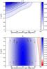 |
Fig. 8 Normalised flux πFn (upper panel) and Ps (lower panel) as functions of the planetary phase angle α and wavelength λ for the cloudfree model planet. |
The normalised flux and degree of polarisation of the reflected starlight depend not only on phase angle α, but also on wavelength λ. In Fig. 8 we show πFn and Ps of light that is reflected by a cloudfree (b = 0) planet as functions of α and λ. The atmospheric molecular scattering optical thickness ranges from 1.1 at λ = 0.3 μm to 0.009 at λ = 1.0 μm. Clearly, πFn is largest at the smallest values of λ and α, where the atmospheric optical thickness is largest and where most of the illuminated hemisphere of the planet is visible, and decreases smoothly with increasing λ and α. The degree of polarisation Ps shows the strong maximum around α = 90° that is due to Rayleigh scattering. The general increase of Ps with λ is due to the decrease of the atmospheric optical thickness, and hence the multiple scattering which usually decreases Ps, with λ. The decrease of the atmospheric optical thickness also explains why the phase angle region where Ps is negative narrows with increasing λ: the smaller the optical thickness, the longer the path through the atmosphere, and hence the larger the phase angle required to have enough second order scattered light to change the sign of Ps.
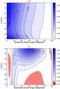 |
Fig. 9 Similar to Fig. 8, except for a model planet with a cloud layer with b = 10.0 (at λ = 0.55 μm) with its top at 0.628 bar that is composed of model A particles (reff = 2.0 μm). |
Figure 9 is similar to Fig. 8 except for an atmosphere that contains a cloud layer composed of model A particles, with b = 10.0 (at λ = 0.55 μm), and with its top at 0.628 bar. The cloud layer strongly increases πFn, except at large values of α, where the observed light has not penetrated deep enough into the atmosphere to encounter the cloud. The features seen at α ≈ 10° were also seen in Fig. 7, and trace back to the single scattering features at Θ ≈ 170° in Fig. 3. Like in Fig. 7, the primary rainbow is hardly visible in the fluxes shown in Fig. 9.
Adding a cloud layer to the model atmosphere strongly decreases Ps, especially at longer wavelengths, as can be seen from comparing Figs. 9 and 8. At the shortest wavelengths, the Rayleigh scattering maximum of Ps (around α = 90°) is still visible, because there, the molecular scattering optical thickness above the cloud layer is still significant. With increasing λ, this optical thickness decreases, and the contribution of light that is reflected by the cloud layer increases. In particular, the ridge in Ps near α = 35° at 0.5 μm and extending towards α = 25° at 1.0 μm, is the primary rainbow. The strength of this rainbow decreases with increasing λ, from about 0.15 (15%) at λ = 0.3 μm to about 0.07 (7%) at λ = 1.0 μm.
The branch of negative values of Ps in Fig. 9 that appears from λ = 0.4 to 0.85 μm for α ≲ 20°, corresponds to the branch of negative values of Ps for light that has been single scattered by the model A cloud particles for 150° < Θ < 180° (see Fig. 4). The negative values of Ps in Fig. 9 that appear for λ > 0.7 μm and for intermediate phase angles are related to the band of negative values of the single scattering Ps for Θ < 90° (see Fig. 4).
5.2. The effects of the cloud particle sizes
To study the effects of the cloud particle sizes on πFn and Ps of the reflected starlight, we replace the model A particles in our cloud layer with model B particles, while keeping the cloud top pressure at 0.628 bar and its optical thickness b equal to 10 (at λ = 0.55 μm). The resulting πFn and Ps are shown in Fig. 10. For comparison, Fig. 11 shows a cross-section of Figs. 9 and 10 at a phase angle of 90°, and includes lines for clouds composed of model A2 particles.
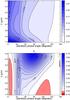 |
Fig. 10 Similar to Fig. 9, except for a cloud layer that is composed of model B particles (reff = 6.0 μm). |
Comparing Figs. 10 and 9, we can see that the introduction of the larger cloud particles in our model atmosphere leaves clear traces in the reflected πFn and Ps. Figure 11 shows, for α = 90°, that the effect of the cloud particle variance on πFn and Ps is negligibly small. Indeed, the particle effective radius appears to be the parameter that influences the reflected signals most.
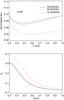 |
Fig. 11 Cross-sections through Figs. 9 and 10 at α = 90° to show the spectral effects of the particle size on the reflected normalised flux and degree of polarisation: model A particles (black, solid line; Fig. 9), and model B particles (red, dot-dashed line; Fig. 10). Also included: model A2 particles (blue, triple-dot-dashed line). |
In Figs. 10 and 9, normalised flux πFn is significantly lower with the larger particles except for the largest values of λ and α. The lower values of πFn are explained by the smaller single scattering albedo of the model B cloud particles (see Fig. 2). Indeed, while the albedo of the model A particles equals ~1 across the wavelength range under consideration, the albedo of the model B particles varies from 0.84 at 0.3 μm, to 0.90 at 0.55 μm, and 0.94 at 1.0 μm. The differences between the reflected normalised fluxes at the largest phase angles are relatively small, because there, most of the reflected starlight has been scattered in the layers above the cloud.
With the model B cloud particles, πFn of the light that is reflected by the planet shows a somewhat stronger primary rainbow than with the smaller model A particles (Fig. 9). This is explained by the difference in strength of the primary rainbow in the single scattering phase functions of both particle types (Fig. 3).
With the model B cloud particles (Fig. 10), Ps shows stronger angular features than with the smaller model A particles (Fig. 9). In particular, the maximum around α = 90° is higher, which is due to the lower single scattering albedo of the model B particles: because more light is absorbed within the cloud layer, there is less multiple scattering, and less (little polarised) light is scattered upward by the cloud layer. With increasing λ, the maximum in Ps shifts towards smaller phase angles, because there the Rayleigh scattering feature blends with the strong features in the single scattering Ps of the model B particles that can be seen for Θ > 100° in Figs. 3 and 5.
Furthermore, as expected from the single scattering polarisation phase function (Fig. 3), and as in the case of πFn, the primary rainbow is a much more prominent feature in Ps of the reflected starlight with the model B particles, than with the model A particles. In particular, at λ = 0.55 μm, with the model A particles, Ps in the rainbow is about 0.12, while with the model B particles, Ps in the rainbow reaches a value as high as 0.26. The latter value is comparable to the case in which the atmosphere contains a cloud layer of model A particles with an optical thickness of only b = 0.5 (see Fig. 7). In observations, the two cases should be separable because with the model B particles, the primary rainbow peak is the global maximum across the entire α regime, while in the case of the thinner cloud made out of model A particles, it is just a local maximum, since Ps in the Rayleigh scattering peak is as large as 0.44.
5.3. The effects of the cloud top pressure
To study the effects of the cloud top pressure on πFn and Ps, we use a cloud composed of model A particles, with b = 10 (at λ = 0.55 μm), and place it with its top at three different pressures ptop in the model atmosphere. The geometrical thickness of each cloud is 1 km. We use a low cloud, with ptop = 0.802 bar (corresponding to 2 km on Earth), a middle cloud, with ptop = 0.710 bar (3 km on Earth), and a high cloud, with ptop = 0.628 bar (4 km on Earth). The corresponding cloud top temperatures on Earth are 285, 279, and 273 K, respectively (see Table 1). These cloud top pressures are chosen to correspond with terrestrial liquid water clouds.
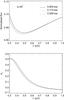 |
Fig. 12 Normalised flux πFn (upper panel) and Ps (lower panel) as functions of the wavelength λ for model planets with cloud layers with cloud top pressures ptop equal to 0.802 bar (solid line), 0.710 bar (dashed line) and 0.628 bar (dashed-dotted line). The cloud layer has an optical thickness b = 10 (at 0.55 μm), and is composed of model A particles. The planetary phase angle α is 90°. |
Figure 12 shows πFn and Ps as functions of λ, at α = 90°, for the three values of ptop. At wavelengths shorter than about 0.6 μm, πFn increases with increasing ptop, because of the increasing amount of gaseous molecules, and hence molecular scattering optical thickness, above of the cloud layer. With increasing wavelength, the sensitivity of πFn to ptop vanishes, because of the decreasing molecular scattering optical thickness above the cloud layer. The increase of πFn with increasing λ that occurs for all three values of ptop is due to the corresponding increase of the scattering optical thickness of the cloud layer and the decrease of its absorption optical thickness (see Fig. 2).
As can be seen in Fig. 12, Ps increases with increasing ptop at almost all wavelengths, because of the increasing amount of molecules, which scatter light with a relatively high degree of polarisation, above the cloud layer. In Fig. 12, the largest increase in Ps is 0.044 at λ = 0.44 μm when ptop increases from 0.628 bar to 0.802 bar. The change of Ps with ptop vanishes at the shortest and longest wavelengths. When λ ≲ 0.32 μm, Ps actually decreases slightly with increasing ptop, because here the increasing amount of molecules leads to an increase of multiple scattered, little polarised light. At the longest wavelengths, the molecular scattering optical thickness of the atmosphere above the cloud layer is too small for each of the three values of ptop to significantly influence Ps.
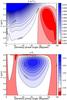 |
Fig. 13 Differences πFn(ptop = 0.802) − πFn(ptop = 0.628) (upper panel) and Ps(ptop = 0.802) − Ps(ptop = 0.628) (lower panel) as functions of λ and α for a model planet with a cloud layer with b = 10 (at λ = 0.55 μm) that is composed of model A particles. |
The dependence of πFn and Ps on ptop varies not only with λ, but also with α. In Fig. 9, we presented πFn and Ps as functions of α and λ for a cloud layer with ptop = 0.628 bar. To get a better view of the change of πFn and Ps with ptop, Fig. 13 shows πFn(ptop = 0.802) − πFn(ptop = 0.628) and Ps(ptop = 0.802) − Ps(ptop = 0.628) as functions of α and λ. As can be seen in Fig. 13, πFn increases with increasing ptop, except for α ≳ 110° and λ ≳ 0.32 μm. The changes of πFn with ptop from 0.802 to 0.628 bar are very small: at maximum ~3.3% for λ = 0.3 μm and α ~ 10°. In particular at the phase angles around 90°, where an exoplanet will be easiest to observe directly because it will be relatively far from its star, the sensitivity of πFn to ptop is extremely small, making the derivation of cloud top pressures in this range using flux measurements practically impossible.
Regarding the polarisation plot of Fig. 13, increasing ptop yields the largest increases in Ps for  m and α ≈ 90°. As was also explained for Fig. 12, Ps increases with increasing ptop because of the increase of the amount of molecules above the cloud layer. In particular, the largest change in Ps is 0.05, at λ = 0.44 μm and α = 94°.
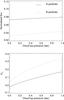 |
Fig. 14 Normalised flux πFn (upper panel) and Ps (lower panel) at λ = 0.55 μm, as functions of ptop for model cloud layers with b = 10 (at λ = 0.55 μm) that are composed of model A or model B particles. The planetary phase angle α is 90°. |
In Fig. 14, finally, we present πFn and Ps as functions of ptop, for a cloud layer with an optical thickness of 10 (at 0.55 μm), consisting of A or B particles, for λ = 0.55 μm and α = 90°. Not surprisingly, both πFn and Ps vary smoothly with ptop. The normalised flux increases with ptop, for both cloud particle types. In particular, for the model A (B) particles, πFn increases from about 0.072 (0.032) at ptop = 0 bar to 0.079 (0.044) at ptop = 1 bar. At this wavelength, the degree of polarization Ps increases with ptop, as well; for the model A particles, Ps increases from -0.015 at ptop = 0 bar to about 0.17 at ptop = 1 bar, and for the model B particles, Ps increases from 0.045 at ptop = 0 bar to about 0.34 at ptop = 1 bar. The negative values of Ps for the model A particles and ptop < 0.1 bar are explained by the single scattering properties of these particles at Θ = 90° (see Fig. 3).
6. Summary and discussion
We have presented numerically simulated normalised flux (πFn) and polarisation (Ps) spectra from 0.3 to 1.0 μm of exoplanets that are completely covered by liquid water clouds. We studied the effects of the cloud optical thickness, the size of the cloud particles, and the cloud top altitude on the spectra as functions of the planetary phase angle. Knowing the microphysical properties of cloud particle on a planet is important for our understanding of the cloud’s influence on the planetary climate. In particular, from Earth studies we know that the cloud particle sizes strongly influence the cloud radiative forcing (see e.g. Chapman et al. 2009; Kobayashi & Adachi 2009, and references therein), since they change the way cloud particles scatter and absorb incident sunlight and thermal radiation.
Given the huge number of free parameters in systems like this, our aim was not to cover the whole parameter space, but rather to explore the information content of, in particular, the degree of polarisation of starlight that is reflected by a planet, and the spectral and phase angle ranges that would provide this information. Although we used atmospheric temperature and pressure profiles that are typical for an Earth-like planet, our results can also be used to represent liquid water clouds on gaseous planets, except that the cloud top pressures are likely to be different.
The cloud’s optical thickness b strongly influences the normalised flux and polarisation spectra of our model planets. In particular, up to about b = 40, an increase of b leads to an increase of πFn. For larger optical thicknesses, the cloud layer appears to be semi-infinite and the normalised flux spectra no longer change significantly. In polarisation, increasing b lowers the (polarisation) continuum, because it increases the amount of multiple scattered light, with usually a low degree of polarisation, to the total amount of reflected light. While multiple scattering subdues the angular features in the polarisation, even for the largest values of b, Ps as a function of the planetary phase angle still carries the angular features that are representative for light that was singly scattered by the cloud particles in the upper layers of the cloud. In particular, the locations of maxima and so-called zero-points (where Ps equals zero), are characteristic for the particle size, shape, and composition.
Changing the effective radius reff of the size distribution of the water cloud particles changes their single scattering properties, and hence both the normalised flux and polarisation spectra of the reflected starlight. As an example, increasing reff from 2 μm to 6 μm (keeping veff constant), increases Ps by ~ 0.20 in the blue for a cloud with b = 10, a cloud top pressure of 0.628 bar and at α = 90° (Fig. 11). The effective variance veff has an almost negligible effect on the normalised flux and polarisation spectra, and can thus not be derived from such observations.
Because Ps preserves the angular features of the singly scattered light, the detection of the primary rainbow in Ps at planetary phase angles around 30°, would be a clear indicator of the presence of liquid water clouds. This rainbow is present across a wide range of particle sizes, but is only detectable in Ps, not in πFn (rainbows seen ‘in scattered flux’ on the Earth originate in rain droplets, which are much larger than cloud droplets). Interestingly, our simulations show that for small water cloud droplets (1 μm  μm), the dispersion of the polarised “cloud” rainbows is opposite to that found for “rain” rainbows: at λ = 0.56 μm, the maximum of the polarised rainbow is located at α ~ 32° (corresponding to a single scattering angle Θ of 148°), while for λ = 1.0 μm, the largest Ps is found at α ~ 24° (Θ = 156°). For “rain” rainbows, Θ decreases with increasing λ. Our simulations show that the dispersion for the “cloud” rainbows decreases with increasing particle size. Indeed, in case our model cloud consists of the larger model B particles, the maximum polarised rainbow is found at α ~ 38° (Θ = 142°) for λ = 0.56 μm and at α ~ 36° (Θ = 144°) for λ = 1.0 μm (see Fig. 10).
The inverse dispersion of a polarised “cloud” rainbow should be observable for terrestrial clouds, e.g. when measured looking down towards a cloud layer from an airplane. As far as we know, such observations have not been done yet.
In order to use the polarised rainbow feature for determining the composition and shape of cloud particles, an exoplanet should be observed across the appropriate phase angle range (from about 30° to 40°) and with an appropriate angular resolution (about 10°). To also derive the cloud particle size, an angular resolution of a few degrees (2° − 5°) would be required across the rainbow phase angle range. We expect that if an exoplanet were found that could have liquid water clouds and that would be directly observable, a dedicated observing campaign to search for the rainbow would be conceivable.
The strength of rainbows and other angular features will depend slightly on the cloud top altitude, because the latter is related to the scattering optical thickness of the gaseous atmosphere above the clouds. Our simulations show that the lower the cloud (hence the larger the cloud top pressure), the larger the reflected πFn (in the absence of gaseous absorption). The increase of πFn with decreasing cloud top altitude decreases with increasing wavelength: above about 0.6 μm, πFn appears to be independent of the cloud top altitude. This is due to the decrease of the molecular scattering cross-section, hence the gaseous scattering optical thickness, with increasing wavelength. The sensitivity of πFn depends strongly on the planetary phase angle. In particular, around α = 90°, the sensitivity is very small: πFn changes by at most ~ 1% for a cloud top pressure increase of the order of ~ 0.17 bar (on Earth, this corresponds to a cloud top altitude drop of ~ 2 km). The sensitivity of πFn to the cloud top altitude seems to increase slightly with decreasing phase angle. However, with decreasing phase angle, the difficulty for measuring the normalised flux that is reflected by the planet increases because of the interfering starlight.
The degree of polarisation of the reflected starlight is most sensitive to the cloud top altitude at wavelengths between 0.4 and 0.5 μm, and around α = 90°. Around this phase angle and wavelength range, Ps shows a maximum due to Rayleigh scattered light, and increasing the cloud top pressure (lowering the cloud) leads to an increase of Ps, because of the increase of light that has been singly scattered by the gas molecules above the cloud. In this regime, increasing the cloud top pressure by ~ 0.18 bar, typically increases Ps by 0.05 (5%). At shorter wavelengths, multiple Rayleigh scattering is significant, and increasing the cloud top pressure results in an increase of multiple scattering and hence a (small) decrease of Ps. At longer wavelengths, the gaseous scattering optical thickness is too small to change Ps significantly.
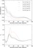 |
Fig. 15 The normalised flux (πFn) and degree of polarisation (Ps) of starlight reflected by a planet covered by two cloud layers; the lower (upper) one composed of model particles B (A). The top of the upper cloud is at 0.628 bar, and for these calculations, the cloud layers themselves do not contain any gas molecules. The lines pertain to different combinations of cloud optical thicknesses (at 0.55 microns): upper cloud b2 = 0.5, lower cloud b1 = 1.5 (orange, dashed-tripple-dotted line); upper cloud b2 = 1.0, lower cloud b1 = 1.0 (black, solid line); upper cloud b2 = 1.5, lower cloud b1 = 0.5 (green, long-dashed line). For comparison, we also included the cases in which both cloud layers contain particles B with total b1 = 2.0 (red, dashed line), and particles A with total b2 = 2.0 (blue, dashed-dotted line). |
7. Future work
The simulated signals that we showed in this paper all pertain to planets with a homogeneous cloud layer, i.e. there are no variations in cloud particle composition and/or size and/or shape in the clouds. In real planetary atmospheres, we expect variations. On Earth, for example, particle sizes usually show some variation with altitude within the cloud. Such variations could influence the retrieval of cloud particle properties and should be investigated. As an example, in Fig. 15, we show πFn and Ps of starlight reflected by a model planet covered by two homogeneous cloud layers on top of each other. The lower cloud layer contains model B particles and has its top at 0.710 bar and the upper cloud layer contains model A particles and its top is located at 0.628 bar. For comparison, we also show πFn and Ps for the cases in which both layers contain particles B or A, respectively. The total optical thickness of the two cloud layers is 2.0 (at λ = 0.55 μm) for each case, but the ratio of the optical thicknesses of the two layers varies.
The curves in Fig. 15 clearly show that even when the upper cloud has a relatively small optical thickness, Ps of the planet is mainly determined by the properties of the upper cloud particles. This is due to the fact that the angular features of Ps are mostly due to singly scattered light, which originates mostly in the upper part of a cloud. Combining polarisation observations at a range of wavelengths, e.g. from the UV to the near-infrared, or even the infrared (where polarisation signatures would be due to scattered thermal radiation), would probably help probing various depths in the cloud layers, since cloud optical thicknesses depend on the wavelength.
Another interesting extension to the work presented in this paper, would be to study the influence of variations in particle shape within the clouds. In this paper, we placed the clouds at altitudes where the ambient temperatures ensure that the cloud particles are liquid, and hence, spherical in shape. With increasing cloud top altitude and decreasing ambient temperatures, clouds will contain more and more ice particles. The single scattering flux and polarisation phase functions of ice cloud particles will differ strongly from those of liquid water particles because of the non-spherical, possibly crystalline shape of the ice particles. We can thus expect that ice particles will significantly influence the polarisation spectrum of a cloudy planet. Using Earth-observation data, Goloub et al. (2000) showed that the strength of the primary rainbow polarisation peak that is characteristic for liquid water cloud particles decreases when the column number density of overlaying ice particles increases. For a full retrieval of cloud parameters, we will thus have to take into account the polarisation characteristics of ice particles. Knowledge of the phase (liquid or solid) of cloud particles gives valuable information on the ambient atmospheric temperatures, especially when combined with knowledge of cloud top altitudes. Flux and polarisation signatures of ice and mixed clouds will be the subject of further study.
Furthermore, the model planets that we used in this paper have horizontally homogeneous atmospheres. We will adapt our numerical radiative transfer and disk integration code to investigate the influence of horizontally inhomogeneities of cloud layers (e.g. partial cloud coverage or Jupiter-like cloud belts and zones) on the flux and polarisation spectra, and on the retrieved cloud parameters.
References
- Adam, J. A. 2002, Phys. Rep., 356, 229 [NASA ADS] [CrossRef] [Google Scholar]
- Bailey, J. 2007, Astrobiology, 7, 320 [NASA ADS] [CrossRef] [PubMed] [Google Scholar]
- Bates, D. R. 1984, Planet. Space Sci., 32, 785 [NASA ADS] [CrossRef] [Google Scholar]
- Cash, W., & New Worlds Study Team 2010, in ASP Conf. Ser. 430, ed. V. Coudé Du Foresto, D. M. Gelino, & I. Ribas, 353 [Google Scholar]
- Cess, R. D., Kwon, T. Y., Harrison, E. F., et al. 1992, J. Geophys. Res., 97, 7613 [NASA ADS] [Google Scholar]
- Chapman, E. G., Gustafson, Jr., W. I., Easter, R. C., et al. 2009, Atm. Chem. Phys., 9, 945 [NASA ADS] [CrossRef] [Google Scholar]
- Daimon, M., & Masumura, A. 2007, Appl. Opt., 46, 3811 [NASA ADS] [CrossRef] [PubMed] [Google Scholar]
- Dave, J. V. 1969, Appl. Opt., 8, 155 [NASA ADS] [CrossRef] [PubMed] [Google Scholar]
- de Haan, J. F., Bosma, P. B., & Hovenier, J. W. 1987, A&A, 183, 371 [NASA ADS] [Google Scholar]
- de Rooij, W. A., & van der Stap, C. C. A. H. 1984, A&A, 131, 237 [NASA ADS] [Google Scholar]
- Fischer, J., & Grassl, H. 1991, J. Appl. Meteor., 30, 1245 [Google Scholar]
- Garay, M. J., de Szoeke, S. P., & Moroney, C. M. 2008, J. Geophys. Res. (Atmospheres), 113, 18204 [NASA ADS] [CrossRef] [Google Scholar]
- Goloub, P., Herman, M., Chepfer, H., et al. 2000, J. Geophys. Res., 105, 14747 [NASA ADS] [CrossRef] [Google Scholar]
- Han, Q., Rossow, W. B., & Lacis, A. A. 1994, J. Clim., 7, 465 [NASA ADS] [CrossRef] [Google Scholar]
- Hansen, J. E., & Hovenier, J. W. 1974, J. Atm. Sci., 31, 1137 [NASA ADS] [CrossRef] [Google Scholar]
- Hansen, J. E., & Travis, L. D. 1974, Space Sci. Rev., 16, 527 [NASA ADS] [CrossRef] [Google Scholar]
- Hovenier, J. W. 1970, A&A, 7, 86 [NASA ADS] [Google Scholar]
- Hovenier, J. W., & Stam, D. M. 2007, J. Quant. Spect. Rad. Trans., 107, 83 [Google Scholar]
- Hovenier, J. W., Van der Mee, C., & Domke, H. 2004, Transfer of polarized light in planetary atmospheres: basic concepts and practical methods, Astrophys. Space Sci. Lib., 318 [Google Scholar]
- Kaltenegger, L., Traub, W. A., & Jucks, K. W. 2007, ApJ, 658, 598 [NASA ADS] [CrossRef] [Google Scholar]
- Kasting, J. F., Whitmire, D. P., & Reynolds, R. T. 1993, Icarus, 101, 108 [NASA ADS] [CrossRef] [PubMed] [Google Scholar]
- Keller, C. U. 2006, in SPIE Conf., 6269 [Google Scholar]
- Keller, C. U., Schmid, H. M., Venema, L. B., et al. 2010, in SPIE Conf., 7735 [Google Scholar]
- Kemp, J. C., Henson, G. D., Steiner, C. T., & Powell, E. R. 1987, Nature, 326, 270 [NASA ADS] [CrossRef] [Google Scholar]
- Kim, D., & Ramanathan, V. 2008, J. Geophys. Res. (Atmospheres), 113, 2203 [NASA ADS] [CrossRef] [Google Scholar]
- Klouda, G. A., Lewis, C. W., Rasmussen, R. A., et al. 1996, Env. Sci. Technol., 30, 1098 [CrossRef] [Google Scholar]
- Kobayashi, T., & Adachi, A. 2009, EGU General Assembly 2009, held 19−24 April, in Vienna, Austria, 11, 11842 [Google Scholar]
- Liou, K. N., & Takano, Y. 2002, Geophys. Res. Lett., 29, 090000 [Google Scholar]
- Malek, E. 2007, AGU Fall Meeting Abstracts, A18 [Google Scholar]
- Marley, M. S., Gelino, C., Stephens, D., Lunine, J. I., & Freedman, R. 1999, ApJ, 513, 879 [NASA ADS] [CrossRef] [Google Scholar]
- Martin, G. M., Johnson, D. W., & Spice, A. 1994, J. Atm. Sci., 51, 1823 [NASA ADS] [CrossRef] [Google Scholar]
- Matcheva, K. I., Conrath, B. J., Gierasch, P. J., & Flasar, F. M. 2005, Icarus, 179, 432 [NASA ADS] [CrossRef] [Google Scholar]
- Mayor, M., & Queloz, D. 1995, Nature, 378, 355 [NASA ADS] [CrossRef] [Google Scholar]
- McClatchey, R. A., Fenn, R., Selby, J. E. A., Volz, F., & Garing, J. S. 1972, AFCRL-72.0497 (US Air Force Cambridge research Labs) [Google Scholar]
- Minnis, P., Heck, P. W., Young, D. F., Fairall, C. W., & Snider, J. B. 1992, J. Appl. Meteor., 31, 317 [NASA ADS] [CrossRef] [Google Scholar]
- Mishchenko, M. I., Rosenbush, V. K., Kiselev, N. N., et al. 2010 [arXiv:1010.1171] [Google Scholar]
- Oakley, P. H. H., & Cash, W. 2009, ApJ, 700, 1428 [NASA ADS] [CrossRef] [Google Scholar]
- Peralta, J., Hueso, R., & Sánchez-Lavega, A. 2007, Icarus, 190, 469 [NASA ADS] [CrossRef] [Google Scholar]
- Pope, R. M., & Fry, E. S. 1997, Appl. Opt., 36, 8710 [NASA ADS] [CrossRef] [PubMed] [Google Scholar]
- Pour Biazar, A., McNider, R. T., Doty, K., & Cameron, R. 2007, AGU Fall Meeting Abstracts, D740 [Google Scholar]
- Ramanathan, V., Barkstrom, B. R., & Harrison, E. F. 1989, Phys. Today, 42, 22 [NASA ADS] [CrossRef] [Google Scholar]
- Saar, S. H. & Seager, S. 2003, in Scientific Frontiers in Research on Extrasolar Planets, ed. D. Deming, & S. Seager, ASP Conf. Ser., 294, 529 [Google Scholar]
- Seager, S., Whitney, B. A., & Sasselov, D. D. 2000, ApJ, 540, 504 [NASA ADS] [CrossRef] [Google Scholar]
- Segal, Y., & Khain, A. 2006, J. Geophys. Res. (Atmospheres), 111, 15204 [NASA ADS] [CrossRef] [Google Scholar]
- Stam, D. M. 2003, in Earths: DARWIN/TPF and the Search for Extrasolar Terrestrial Planets, ed. M. Fridlund, T. Henning, & H. Lacoste, ESA SP, 539, 615 [Google Scholar]
- Stam, D. M. 2008, A&A, 482, 989 [NASA ADS] [CrossRef] [EDP Sciences] [Google Scholar]
- Stam, D. M., Hovenier, J. W., & Waters, L. B. F. M. 2004, A&A, 428, 663 [NASA ADS] [CrossRef] [EDP Sciences] [Google Scholar]
- Stam, D. M., de Rooij, W. A., Cornet, G., & Hovenier, J. W. 2006, A&A, 452, 669 [NASA ADS] [CrossRef] [EDP Sciences] [MathSciNet] [Google Scholar]
- Stephens, G. L., Vane, D. G., Tanelli, S., et al. 2008, J. Geophys. Res. (Oceans), 113, [Google Scholar]
- Tinetti, G., Rashby, S., & Yung, Y. L. 2006, ApJ, 644, L129 [NASA ADS] [CrossRef] [Google Scholar]
- van de Hulst, H. C. 1957, Light Scattering by Small Particles (New York: John Wiley & Sons) [Google Scholar]
- van Deelen, R., Hasekamp, O. P., van Diedenhoven, B., & Landgraf, J. 2008, J. Geophys. Res. (Atmospheres), 113, 12204 [NASA ADS] [CrossRef] [Google Scholar]
- van Diedenhoven, B., Hasekamp, O. P., & Landgraf, J. 2007, J. Geophys. Res. (Atmospheres), 112, 15208 [NASA ADS] [CrossRef] [Google Scholar]
- Wark, D. Q., & Mercer, D. M. 1965, Appl. Opt., 4, 839 [NASA ADS] [CrossRef] [Google Scholar]
- Weigelt, A., Hermann, M., van Velthoven, P. F. J., et al. 2009, J. Geophys. Res. (Atmospheres), 114, 1204 [NASA ADS] [CrossRef] [Google Scholar]
- Yamamoto, G., & Wark, D. Q. 1961, J. Geophys. Res., 66, 3596 [NASA ADS] [CrossRef] [Google Scholar]
All Tables
The altitude (in km), pressure (in bar), and temperature (in K) at the bottom and top of each layer of our model atmosphere (McClatchey et al. 1972).
The effective radius reff (in μm) and variance veff of the standard size distributions (see Hansen & Travis 1974, and Eq. (15)) that describe our model cloud particles.
All Figures
|
Fig. 1 Particle size distributions (see Eq. (8)) for model A particles (reff = 2.0 μm, veff = 0.1; red, dashed line) and model B particles (reff = 6.0 μm, veff = 0.4; black, solid line). Each size distribution has been normalised such that the integral over all sizes equals 1. |
| In the text | |
|
Fig. 2 Spectral variation of the absorption (upper panel) and scattering (lower panel) optical thicknesses, babs and bsca, of cloud layers composed of the following model particles (see Table 2): A (reff = 2.0 μm, veff = 0.1; black, solid line), A2 (reff = 2.0 μm, veff = 0.4; blue, dashed–dotted line), B (reff = 6.0 μm, veff = 0.4; red, dashed line), and B2 (reff = 6.0 μm, veff = 0.1; orange, dashed–tripple–dotted line). The total optical thickness (b = bsca + babs) of each cloud layer is 2.0 at λ = 0.55 μm. |
| In the text | |
|
Fig. 3 Phase function on a logarithmic scale (upper panel) and degree of polarisation Ps (lower panel) for incident unpolarised light at λ = 0.55 μm that is singly scattered by our model water cloud particles (see Table 2) as functions of the scattering angle Θ: model A (black, solid lines), model B (red, dashed lines), model A2 (blue, dashed-dotted lines) and model B2 (orange, dashed-triple-dotted lines). For comparison, the phase function and Ps are also shown for gas molecules (i.e. Rayleigh scattering) (purple, long-dashed lines). |
| In the text | |
|
Fig. 4 Phase function on a logarithmic scale (upper panel) and degree of polarisation Ps (lower panel) for incident unpolarised, singly scattered light as functions of the scattering angle Θ and the effective size parameter xeff = 2πreff/λ for model cloud particles with veff = 0.1, i.e. models A and B2. For model A (with reff = 2.0 μm), the curves shown in Fig. 3 correspond to xeff = 23, while for model B2 (with reff = 6.0 μm), they correspond to xeff = 69. |
| In the text | |
|
Fig. 5 Similar to Fig. 4, except for particles with veff = 0.4, i.e. models A2 and B. For model A2 (with reff = 2.0 μm), the curves shown in Fig. 3 correspond to xeff = 23, while for model B (with reff = 6.0 μm), they correspond to xeff = 69. |
| In the text | |
|
Fig. 6 Scattering angle Θ where the primary rainbow in Ps occurs as a function of the wavelength for the model A (reff = 2.0 μm) and B2 (reff = 6.0 μm) particles. |
| In the text | |
|
Fig. 7 Normalised flux πFn (upper panel) and Ps (lower panel) at λ = 0.55 μm, as functions of the planetary phase angle α for model planets with a cloudfree atmosphere (black solid line) and with atmospheres containing a cloud layer ranging from 3 to 4 km, composed of model A cloud particles, with the following cloud optical thicknesses b (at λ = 0.55 μm): 0.5 (red, dashed lines), 1.0 (green, dash-dotted lines), 10.0 (blue, dash-triple-dotted lines), 20.0 (orange, long-dashed lines), 40.0 (pink, diamond lines), and 60.0 (purple, cross lines). |
| In the text | |
|
Fig. 8 Normalised flux πFn (upper panel) and Ps (lower panel) as functions of the planetary phase angle α and wavelength λ for the cloudfree model planet. |
| In the text | |
|
Fig. 9 Similar to Fig. 8, except for a model planet with a cloud layer with b = 10.0 (at λ = 0.55 μm) with its top at 0.628 bar that is composed of model A particles (reff = 2.0 μm). |
| In the text | |
|
Fig. 10 Similar to Fig. 9, except for a cloud layer that is composed of model B particles (reff = 6.0 μm). |
| In the text | |
|
Fig. 11 Cross-sections through Figs. 9 and 10 at α = 90° to show the spectral effects of the particle size on the reflected normalised flux and degree of polarisation: model A particles (black, solid line; Fig. 9), and model B particles (red, dot-dashed line; Fig. 10). Also included: model A2 particles (blue, triple-dot-dashed line). |
| In the text | |
|
Fig. 12 Normalised flux πFn (upper panel) and Ps (lower panel) as functions of the wavelength λ for model planets with cloud layers with cloud top pressures ptop equal to 0.802 bar (solid line), 0.710 bar (dashed line) and 0.628 bar (dashed-dotted line). The cloud layer has an optical thickness b = 10 (at 0.55 μm), and is composed of model A particles. The planetary phase angle α is 90°. |
| In the text | |
|
Fig. 13 Differences πFn(ptop = 0.802) − πFn(ptop = 0.628) (upper panel) and Ps(ptop = 0.802) − Ps(ptop = 0.628) (lower panel) as functions of λ and α for a model planet with a cloud layer with b = 10 (at λ = 0.55 μm) that is composed of model A particles. |
| In the text | |
|
Fig. 14 Normalised flux πFn (upper panel) and Ps (lower panel) at λ = 0.55 μm, as functions of ptop for model cloud layers with b = 10 (at λ = 0.55 μm) that are composed of model A or model B particles. The planetary phase angle α is 90°. |
| In the text | |
|
Fig. 15 The normalised flux (πFn) and degree of polarisation (Ps) of starlight reflected by a planet covered by two cloud layers; the lower (upper) one composed of model particles B (A). The top of the upper cloud is at 0.628 bar, and for these calculations, the cloud layers themselves do not contain any gas molecules. The lines pertain to different combinations of cloud optical thicknesses (at 0.55 microns): upper cloud b2 = 0.5, lower cloud b1 = 1.5 (orange, dashed-tripple-dotted line); upper cloud b2 = 1.0, lower cloud b1 = 1.0 (black, solid line); upper cloud b2 = 1.5, lower cloud b1 = 0.5 (green, long-dashed line). For comparison, we also included the cases in which both cloud layers contain particles B with total b1 = 2.0 (red, dashed line), and particles A with total b2 = 2.0 (blue, dashed-dotted line). |
| In the text | |
Current usage metrics show cumulative count of Article Views (full-text article views including HTML views, PDF and ePub downloads, according to the available data) and Abstracts Views on Vision4Press platform.
Data correspond to usage on the plateform after 2015. The current usage metrics is available 48-96 hours after online publication and is updated daily on week days.
Initial download of the metrics may take a while.