| Issue |
A&A
Volume 529, May 2011
|
|
|---|---|---|
| Article Number | A98 | |
| Number of page(s) | 9 | |
| Section | Numerical methods and codes | |
| DOI | https://doi.org/10.1051/0004-6361/201116540 | |
| Published online | 11 April 2011 | |
Extensions and applications of the iterative method
1
Laboratoire d’Astrophysique de Marseille (LAM), UMR6110, CNRS/Université de Provence, Technopôle de Marseille-Etoile, 38 rue Frédéric Joliot Curie, 13388 Marseille Cedex 20, France
2
Center de recherche INRIA Bordeaux – Sub-Ouest, Bordeaux, 351 Course de la Libération, France
3
Sobolev Astronomical Institute, St. Petersburg State University, Universitetskij pr. 28, 198504 St. Petersburg, Stary Peterhof, Russia
e-mail: This email address is being protected from spambots. You need JavaScript enabled to view it.
Received: 18 January 2011
Accepted: 3 March 2011
Abstract
Aims. We aim to develop an algorithm for constructing equilibrium initial conditions for simulations of disk galaxies with a triaxial halo and/or a gaseous component. This will pave the way for N-body simulations of realistic disk galaxies.
Methods. We use the iterative method, which we presented in a previous article. The idea of this method is very simple. It relies on constrained evolution.
Results. We develop an algorithm for constructing equilibrium models of disk galaxies including a gaseous disk and a triaxial or axisymmetric halo. We discuss two test models. The first model consists of a spherical halo, a stellar disk, and an isothermal gaseous disk. The second model consists of a triaxial halo, a stellar disk, and a star-forming gaseous disk. We demonstrate that both test models are very close to equilibrium, as we had intended.
Key words: galaxies: kinematics and dynamics / methods: numerical
© ESO, 2011
1. Introduction
In this article we consider a method for constructing equilibrium initial conditions for simulations of disk galaxies with a triaxial halo and a gaseous component. N-body systems have the following feature: if we construct some non-equilibrium N-body system and let it evolve, it will reach an equilibrium state fairly fast (on a time scale of a few crossing-times) and this independent of the presence or absence of gas. This, however, does not mean that it is not necessary to construct equilibrium initial conditions. If some initial conditions are constructed by means of a more or less rough approximate method, i.e. out of equilibrium, the system will readjust fairly fast and reach some equilibrium state. But this readjustment will change the mass distribution of the system and its kinematics. This way an equilibrium condition will be obtained, but it will not have the desired parameters, i.e. the desired mass distribution and kinematics. This makes it very difficult or in a strict sense, nearly impossible to study a particular galaxy with a known mass and velocity distributions. Also, when using N-body simulations to study an evolution as a function of a given parameter of the initial configuration, it is necessary to make sure that the chosen parameter does not change considerably during the readjustment to equilibrium, or that at least the sequence of the different models is not readjusted. Furthermore, in some cases the initial violent readjustment to equilibrium could influence the process under study. It is thus preferable to construct initial conditions as close to equilibrium as possible to avoid such problems.
In Rodionov et al. (2009, hereafter RAS09) we presented an iterative method for constructing equilibrium N-body models with given properties, the general idea of which can be applied to an arbitrary dynamical system. The method outlined there can be used for constructing multicomponent axisymmetric models of disk galaxies without gas. Here we will extend this method for models with a gaseous disk and models with a triaxial halo. Other methods for constructing gaseous equilibrium disk models have been proposed. For example Springel et al. (2005) introduced a method in which the gaseous disk was constructed with the help of the equation of hydrostatic equilibrium.
Here, we will use the iterative method to construct the gaseous component because it is conceptually simple, very easy to implement and, as we will demonstrate in this article, gives good results. Furthermore, in this way we are sure that all components are in equilibrium since the iterative method has been used in all cases.
We model the collisionless components with an N-body code and the gas with SPH. We will consider two types of gas. The first type is isothermal gas, which we model by means of the public GADGET2 code (Springel 2005). The second type is a sub-resolution multiphase model for star-forming gas, developed by Springel & Hernquist (2003).
This paper is organized as follows. We first discuss in Sect. 2 the application of the iterative method to the construction of axisymmetrical disk galaxy models with a gaseous disk. In Sect. 3 we demonstrate how to construct such models within triaxial haloes. We briefly conclude in Sect. 4.
2. Axisymmetric models with a gaseous disk
2.1. Equilibrium model of the gaseous disk
The vertical density profile of the gaseous disk cannot be arbitrary. It is governed by the balance between gravity and pressure, i.e. by hydrostatic equilibrium:  (1)where Φ is the total gravitational potential of all components, ρg is the density of the gaseous disk and Pg is the pressure in the gaseous disk. If the equation of state has the given form P = P(ρ), the vertical structure of the gaseous disk is fully determined by Eq. (1) for a given surface density. This last statement is fulfilled for both gaseous models considered here: the isothermal gas and the sub-resolution multiphase model (Springel & Hernquist 2003; Springel et al. 2005). We thus need to construct a model of gaseous disk with a given projected surface density radial profile Σg(R), in equilibrium in a potential that is the sum of its own potential and of a given external potential Φext generated by all other components of the galaxy.
In RAS09 we describe the iterative method that can be used for constructing an equilibrium N-body system with a given mass distribution, following given kinematical constraints. The same conceptually method, with only relatively minor modifications can be applied for the construction of the gaseous disk. It relies on constrained (or guided) evolution. When constructing the equilibrium N-body system, we let it evolve, and during this evolution we fix the desired mass distribution and kinematics (see RAS09). This will be the same for the gaseous disk, except that now we do not fix the full mass distribution, but only the projected surface density.
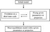 |
Fig. 1 General scheme of the iterative method. |
The general scheme of the iterative method is outlined in Fig. 1. We start from some initial system, which is the starting point of the iterative procedure. We then let the system go through a sequence of evolutionary steps of short duration. At the end of each one of these steps, and before the new evolutionary step is started, we “set” the chosen parameters or quantities to the desired values (see RAS09). We repeat this iteration procedure a number of times, alternating one evolution phase and one phase during which the necessary parameters are set, until we come sufficiently near to the desired equilibrium state. In practice, to apply this general scheme we need to define which initial model we will use, and, most important, which parameters we want to “fix” during the iterative procedure.
Let us now describe how we will apply this iterative method to the construction of an equilibrium gaseous disk. Our initial model is a gaseous disk with a given surface density Σg(R). The vertical coordinates of the particles can be arbitrarily chosen (for example equal to zero). Equally arbitrary, the tangential velocity of each particle is set equal to the circular velocity and the vertical and radial velocities are set equal to zero. The circular velocity is calculated from the total potential, which is the sum of Φext, due to the adopted mass distribution of the collisionless part, and the potential generated by the initial distribution of the gas. At this stage it is not necessary to calculate the circular velocity very accurately. Even if we set the azimuthal velocities equal to twice or to half of the circular velocity, the iterative method will converge to the same result. In the case of a non-isothermal system the thermal energies of the particles can be arbitrarily chosen. This model will be the starting point for the iterative procedure (see Fig. 1). Having thus obtained the starting model, we start the iterative procedure, which consists of a sequence of evolutionary steps of short duration, followed by steps during which some parameters or quantities are fixed, and this until a near equilibrium model is obtained. In this example we fix the following parameters:
-
surface density of the gaseous disk;
-
the condition of axisymmetry.
To fix the surface density in the gaseous disk at the end of an evolutionary step we proceed as follows. We construct a gaseous disk with the desired surface density, but with velocities and vertical coordinates chosen according to the velocities and the vertical coordinates of the disk resulting from the evolution step. We first construct a new gaseous disk with the desired surface density profile. We then “transfer” the velocity distribution and the distribution of the vertical coordinates of the particles from the system obtained from the evolution to this new system, using the “transfer” algorithm described in RAS09 (see Sect. 2.2 in that paper). The basic idea of this algorithm is very simple, namely we assign to the new-model particles the velocities of those particles from the old model that are “nearest” to the ones in the new model, the definition of nearest depending on the problem at hand. In the present case we need to “transfer” the vertical coordinate of the particle together with the velocities. Since our model is axisymmetric, we need to search for the nearest particle in the one-dimensional space R, where R is the cylindrical radius. This implicitly fixes the condition of axisymmetry. The vertical coordinate should not be taken into account during the search for the nearest neighbour because we copy it from the evolved model particle to the new model particle together with the velocities. In the case of non-isothermal gas, the thermal energy of the particle should be copied together with the velocities and the vertical coordinate.
2.2. Equilibrium models of stellar components
The algorithm for constructing the equilibrium N-body system with given parameters and constraints is described in RAS09 and is not altered by the presence of the gaseous component. We simply need to take into account the gravitational acceleration caused by the gaseous component when creating the collisionless components, since it will act on them as an external potential. However, because we initially know only the surface density of the gaseous disk, we cannot calculate the three-dimensional gravitational acceleration. We need, therefore, to construct the equilibrium model of the gaseous disk first, before that of the collisionless components. After constructing this model we have the full mass model of the gaseous disk and can construct all other components of the galaxy, taking into account the acceleration generated by the gaseous disk.
2.3. Technical details
In this section we elaborate a few important technical points, useful to anybody wishing to apply the iteration method.
The iterative method has two free parameters: the duration of each iteration, ti, and the number of neighbours used in the “transfer” algorithm, nnb (see Sect. 2.1 of this paper and Sect. 2.2 of RAS09). The choice of these parameters was discussed in RAS09 Sect. 2.5. We choose both these parameters empirically. In all experiments discussed in this article we use nnb = 10.
We construct each component of the galaxy separately in the rigid potential of all other components. So in the iterative method when we calculate the evolution of the system during the iteration time, we do it in the presence of the appropriative external potential. This can be done either by introducing an analytical external potential, or by adding the component(s) that create this external potential as a rigid N-body system. In the current work we use the latter. For example, to include the external potential due to the halo, we simply add rigid particles to the system according to the mass distribution of the halo.
When creating the collisionless components we follow the evolution using the public version of the gyrfalcon N-body code (Dehnen 2000, 2002). For the gaseous disk we need an appropriate SPH code. For the isothermal gas we use the public version of the GADGET2 code (Springel 2005) and for the multiphase gas code with sub-grid resolution physics we use a private version of GADGET2 kindly provided by Springel and described in Springel & Hernquist (2003).
We still need to decide when the iteration procedure will be stopped. We can assume that the iterative process has converged when the system does not change by more than a pre-set amount during one single iteration. We check this convergence by comparing different parameters of the system in the beginning and in the end of a single short-term evolution step, using a modification of the χ2 test (see Appendix A).
2.4. Example of an axisymmetric model with isothermal gas
In this section we consider an example of a model constructed by means of the method described above. This model is axisymmetric and has an isothermal gaseous disk. It consists of three components: the gaseous disk, the stellar disk, and the halo.
To start, we need to define the mass distribution in both of the non-dissipative components and the projected surface density in the gaseous disk. The stellar disk model is an exponential disk with a density  (2)where Md is the total disk mass, Rd is the disk scale length, zd is its scale height and R is the cylindrical radius. The halo model is a truncated NFW halo (Navarro et al. 1996)
  (3)where rh is the halo scale length, Ch is a parameter defining the mass of the halo and rth is the truncation radius of the halo. Similarly to the stellar disk, the gaseous disk has an exponential projected surface density profile
  (4)where Mg is the total mass of the gaseous disk and Rg is its scale length.
We still need to adopt specific values for the present example. In the above we take Md = 5 × 10¹⁰M⊙, Rd = 3kpc, z0 = 0.6kpc; rh = 12kpc, Ch = 0.0019 × 10¹⁰ M⊙/kpc3, rth = 40kpc; Mg = 0.5 × 10¹⁰M⊙, Rg = 3kpc. We set the temperature of the isothermal gas to T = 10 000K. Note that the mass of the gaseous disk is 10% of the stellar disk mass. For the chosen parameters, the total mass of the halo is Mh ≈ 4.9 × Md. In this specific example we chose Ng = 100 000, Nd = 200 000, Nh = 980 311 for the number of particles in the gaseous disk, the stellar disk, and the halo, respectively. With these numbers, the mass of the particles in the stellar disk and in the halo is the same. We use the GADGET system of units, where the unit of length is ul = 1kpc, the unit of velocity is uv = 1 km s-1, the unit of mass is um = 1010M⊙ and consequently the unit of time is ut ≈ 0.98Gyr. For simplicity, when we convert this time unit into gigayears we assume that ut = 1Gyr.
We also need to select the kinematic constrains for the stellar components (see RAS09). We created the disk with the following velocity dispersion profile  (5)where σR is the radial velocity dispersion. When constructing the halo, we did not impose any specific kinematic constraints. Instead, we aimed for a model not far from isotropic (see RAS09).
As noted in Sect. 2.1, we should first construct the equilibrium model of the gaseous disk with the desired projected surface density embedded in the rigid potential generated by the halo and the stellar disk, as described in Sect. 2.1. To achieve this, we made 50 iterations, each with ti = 0.02Gyr. We note that ti should be shorter than the time scale of the strong instability developing in the system under construction. In our case the gaseous disk forms strong spirals relatively fast (see Fig. 2). It is why we have to choose relatively short ti in this case.
After constructing the equilibrium gaseous disk, we have the full mass model of the galaxy, and we can apply the algorithm for constructing the equilibrium models of the stellar disk and the halo (RAS09).
Let us first describe the stellar disk construction. Our initial model was a cold disk, where all particles move on circular orbits. We made 50 iterations, each with ti = 0.25Gyr. The integration step and softening length were taken dt = 1/210Gyr and ϵ = 0.1kpc, respectively and the tolerance parameter for gyrfalcON was set θt = 0.9. Here we can use relatively low precision because each iteration is short and errors do not accumulate (RAS09). In order to fix the σR(R) profile we applied the algorithm described in RAS09, Sect. 2.3.1, with ndiv = 200 layers. We used the “transvel_cyl” modification of the algorithm of velocity transfer (see RAS09). This algorithm was also used for constructing the halo.
For constructing the halo we also made 50 iterations. The other parameters for this construction were ti = 0.5Gyr, dt = 1/210Gyr, ϵ = 0.1kpc and θt = 0.9. Our initial model was a cold model with velocities equal to zero. During the first 10 iterations we fixed a condition of velocity isotropy (RAS09, 2.3.4), and we did not set any kinematic constraints during the last 40 iterations.
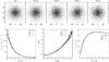 |
Fig. 2 Initial evolutionary stages for the gaseous disk of the constructed disk galaxy model (axisymmetric isothermal case). The evolution of the model was calculated including a live halo and stellar disk. The upper snapshots show the disk views face-on for times 0, 0.1, 0.2, 0.3 and 0.4; the grey intensities correspond to the logarithm of the surface density. The bottom panels show the dependence of various disk quantities on the cylindrical radius R at the same times. Here Σg is the surface density of the gas; z1/2 is the median of the |z| value, i.e a measure of the disk thickness (see Sotnikova & Rodionov 2006) and |

Once all three components of our model were constructed, we simply stacked them to obtain the complete system. To check whether this was indeed near equilibrium, as it should be, we evolved the model using the respective GADGET2 code. The evolution of the gaseous disk over 0.4 Gyr is given in Fig. 2, and shows that the gaseous disk conserves its structural and dynamical properties very well. We also checked the absence of evolution for the stellar disk and the halo. For reasons of conciseness we do not present the corresponding figures here. We conclude that the constructed model is indeed close to equilibrium.
3. Models with triaxial haloes
Here we will describe how to overcome the assumption of axisymmetry and thus to construct equilibrium models with triaxial haloes. Because of the powerful, yet simple basic idea of our iterative method we can remove this assumption relatively easily. As in the axisymmetric case, we will construct each component of the galaxy in the potential of all other components and then will assemble all components together to obtain the final live equilibrium model. We will start from the problem of the construction of equilibrium stellar disk in presence of the external non-axisymmetric potential (created by all other components of the galaxy).
3.1. Construction of the stellar disk in the triaxial external potential
The first problem whose solution is not obvious is deciding which shape the stellar disk should have to be in equilibrium within a triaxial external potential. There are two possibilities. One possibility is to somehow define the shape of the disk and then try to construct an equilibrium model with this shape, i.e. model with given mass distribution. For example, Machado & Athanassoula (2010) obtained an approximate shape of the disk via the epicyclic approximation. This, nevertheless, is only an approximation and there has been no other, more accurate way proposed so far. For this reason, we will let the iterative method itself find the appropriate shape of the disk. We do it in the following way. We do not ask the iterative method to construct a model with a fully defined space distribution of particles. Instead, we fix only the vertical and radial distributions of particles, but not the azimuthal distribution. This means that the R and z coordinates of the particles are defined by a given distribution, but the ϕ coordinate together with velocities is not fixed. The idea described in the last sentence is very similar to the idea of the algorithm we used for constructing the gaseous disk, where we fixed only the surface density (i.e. the radial and azimuthal distribution of particles) but we did not fix the vertical distribution of the particles (see Sect. 2.1). Consequently the algorithm is also very similar to the ones presented in Sect. 2.1.
To apply the general scheme of the iterative method (see Fig. 1) we need to specify an initial model and the parameters which we want to fix during the iterative procedure. Our initial model is an axisymmetric disk with a given radial and vertical distribution. The azimuthal velocity of each particle is set equal to the circular velocity.
With this initial model, we start the iterations, which, as always, consist of a sequence of short time evolutions followed by steps during which we fix the desired parameters or properties (see Fig. 1). In this case we fix the
-
vertical and radial distribution of particles;
-
reflection symmetry about the XZ and YZ planes for the case of system rotating about the z-axis;
-
given profile of σR(R).
There is one potential problem with the symmetry. Indeed, if we fix only the distribution of particles in the vertical and radial directions, then the constructed model can be non-symmetrical in the disk plane. Partially, this is what we aimed for because our target was to avoid axisymmetry. However, even in a triaxial potential we would like the equilibrium model to have a certain level of symmetry and a smooth density distribution. We can enforce our model to have reflection symmetry about the XZ and YZ planes by fixing these symmetries during the iterative procedure (see Fig. 1). But we should take into account that our disk rotates about the z-axis. Reflection symmetry about the XZ plane is fixed by changing the sign of y and vx for all particles with a probability of 1/2. Reflection symmetry about the YZ plane is fixed by changing the sign of x and vy with a probability of 1/2.
Let us note, however, that our experiments show for the stellar disks that fixing this symmetry is not so crucial. In most cases, stellar disks constructed with or without this symmetry are quite similar. Nevertheless, in a few cases disks constructed without imposing this symmetry can be slightly clumpy at the periphery.
Similar to the axisymmetric case, we construct a model with a given σR(R) profile. The value of σR is defined as the radial velocity dispersion of all particles in a cylindrical layer. To fix this value we use the algorithm described in Sect. 2.3.1 of RAS09. However, we note that the physical interpretation of the σR(R) profile in a triaxial case is not so straightforward.
3.2. Construction of the gaseous disk in the triaxial external potential
Here we need to unite the approach discussed in the previous section with the method described in Sect. 2.1. We should allow the gaseous disk more freedom here than in the axisymmetric case, and thus will constrain only the radial distribution of particles (i.e. the radial density profile).
Our initial model is the same as in the axisymmetric case (see Sect. 2.1). During the main part of the iterative procedure (see Fig. 1) we fix the following parameters:
-
radial distribution of particles in the gaseous disk;
-
reflection symmetry about XZ and YZ planes for the case of a system rotating about the z-axis.
The algorithm for fixing reflection symmetries was discussed in the previous subsection. We note, however, that in some cases this algorithm of construction non-axisymmetric gaseous disk may not work very well. The problem is that a reflection symmetry about the XZ and YZ planes does not necessarily imply that the model has a smooth density distribution and for some equations of state the constructed model can have a clumpy density distribution. This can well happen in the case of gas which tends to form clumps very fast. We met this problem when we tried to construct isothermal gaseous disks for temperature of 10 000 K. In this case one can use the old algorithm (Sect. 2.1) and construct an axisymmetrical gaseous disk. Such a disk cannot be in equilibrium in a triaxial external potential, it may, however, be not so far from equilibrium and have a smooth density distribution.
3.3. Construction of the triaxial halo
We need to construct a triaxial halo that should have a given mass distribution and be in equilibrium in a potential consisting of the halo self-potential and the external potential generated by all other components of the galaxy.
The initial model for our iterative method is the halo with the given mass distribution and with arbitrary, e.g., zero velocities. During the main part of the iterative procedure (see Fig. 1) we fix the following parameters:
-
the given mass distribution;
-
reflection symmetry about the XZ and YZ planes for a non-rotating system (see discussion below);
-
during the first 10 iterations we fix a condition of velocity isotropy (see discussion below).
During the first 10 iterations we fix the condition of velocity isotropy. We do it to avoid constructing a model with high velocity anisotropy (see discussion in RAS09 Sect. 3.1).
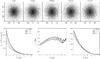 |
Fig. 3 Initial evolutionary stages for the gaseous disk of the constructed disk galaxy model (with triaxial halo and star-forming gas). We show the same quantities as in Fig. 2, except for the bottom right panel, which shows the dependence of the mean thermal energy on R. |
3.4. Construction of the multicomponent system
We will now construct the multicomponent equilibrium model consisting of the triaxial halo and the stellar and gaseous disks. However, we again have the problem that we initially do not know the full three-dimensional mass distribution of the stellar and gaseous disks. We construct each component in the external potential generated by all other components of the galaxy. To construct the gaseous disk we need the final mass distribution in the stellar disk, which we do not have initially, and, moreover, to construct the stellar disk we need the final density distribution in the gaseous disk. However, in both cases (for gaseous and for stellar disks) we fix the radial mass distribution so that the initial axisymmetric disk and the final non-axisymmetric disk have the same radial mass profile. Therefore, the acceleration generated by the initial axisymmetric disk is not so very different from the acceleration generated by the final non-axisymmetric disk. Consequently, even if we construct a stellar disk that is in equilibrium with the initial axisymmetric gaseous disk (and of course with the halo), this disk will be practically in equilibrium with the final non-axisymmetric gaseous disk. But to be sure, we use the following simple two step procedure.
-
1.
Construction of an equilibrium stellar disk in the presence of the initial axisymmetric gaseous disk and halo. Let us call this model D1.
-
2.
Construction of gaseous disk G1 in the presence of D1 and halo.
-
3.
Construction of stellar disk D2 in the presence of G1 and halo.
-
4.
Construction of gaseous disk G2 in the presence of D2 and halo.
-
5.
Construction of the halo in the presence of D2 and G2.
3.5. Example of the model
In this section we discuss the construction of a model of a disk galaxy with a triaxial halo with an axial ratio 1:0.75:0.5 and with a gaseous disk modelled by means of the sub-resolution multiphase model for star-forming gas of Springel & Hernquist (2003). The parameters of the gas that control star formation and feedback were taken from Springel & Hernquist (2003), where these parameters were chosen to fit Kennicut’s law (Kennicutt 1998).
The mass model of the triaxial halo (i.e. the initial model for our iterative procedure) is constructed in the following way. We take a spherical halo and squeeze it along the Y and Z axes by multiplying the y-coordinate and z-coordinate of each particle by b = 0.75 and c = 0.5, respectively. The initially spherical haloes have the density profile described in Hernquist (1993), namely  (6)where Mh is the mass of the halo, γ is the core radius and rc is the cutoff radius. The normalization constant α is defined by
 ![Mathematical equation: \begin{equation} \alpha = \{ 1 - \sqrt{\pi} q \exp{(q^{2})} [1- \textrm{erf}(q)] \}^{-1} , \end{equation}](/articles/aa/full_html/2011/05/aa16540-11/aa16540-11-eq82.png) (7)where q = γ/rc (Hernquist 1993). In the model presented here Mh = 25 × 1010M⊙, γ = 1.5kpc and rc = 30kpc.
(7)where q = γ/rc (Hernquist 1993). In the model presented here Mh = 25 × 1010M⊙, γ = 1.5kpc and rc = 30kpc.
We obtain the initial mass model for the stellar disk as in the previous axisymmetric example. The initial model of the gaseous disk has the surface density profile (4) with parameters Rg = 3kpc and Mg = 1 × 10¹⁰M⊙, i.e. this model has a gaseous component twice as massive as the previous one. The number of particles for the gaseous and stellar disks and for the halo are Ng = 200 000, Nd = 200 000, Nh = 1 000 000, respectively. We note that initially the stellar and gaseous disks are axisymmetric, but during the iterative procedure the azimuthal distribution of particles can be changed, so disks can become non-axisymmetric.
Following the procedure described in Sect. 3.4, we make 100 iterations to construct the stellar disk D1, 50 iterations to construct the gaseous disk G1, 10 iterations to construct D2 and G2, and 50 iterations for the halo. All other parameters of the iterative procedure are the same as in the previous example. But we note that to calculate the evolution of the gaseous disk during the iterative process we use the corresponding GADGET2 with star formation and feedback.
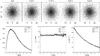 |
Fig. 4 Initial evolutionary stages for the stellar disk of the constructed disk galaxy model (with triaxial halo and star-forming gas). The upper snapshots show the disk viewed face-on for times 0, 0.1, 0.2, 0.3 and 0.4; the grey intensities correspond to the logarithms of particle number density. The bottom panels show the dependence of various disk quantities on the cylindrical radius R at the same times. Here n is the number of particles in concentric cylindrical layers; z1/2 is the median of the value |z|, and σR is the radial velocity dispersion. |
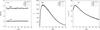 |
Fig. 5 Initial evolutionary stages for the halo of the constructed disk galaxy model (with triaxial halo and star-forming gas). We show the dependence of various quantities on the spherical radius r for various moments of time, a) shows radial profiles of axial ratios b/a and c/a. These profiles were calculated by means of the method described in Machado & Athanassoula (2010); b) shows the profile of the number of particles n in concentric spherical layers; c) shows the profile of the radial velocity dispersion. |
As in the previous case, we check the equilibrium of the constructed model. The evolution of the gaseous disk over 0.4 Gyr is shown in Fig. 3. It is clear that the surface density of the gaseous disk is gradually decreasing because of star-formation. At the same time, the thickness of the gaseous disk and the mean thermal energy are also gradually diminished. But this evolution of the gaseous disk is fairly slow. In Fig. 4 we show the evolution of the stellar disk on a time scale of 0.4 Gyr. It demonstrates that the stellar disk is very close to equilibrium. There is absolutely no sign of initial adjustment to equilibrium. But we note that this stellar disk will form a bar after 2 Gyr of evolution. Figure 5 shows that the halo did not change its properties during the first gigayear of the evolution, and that it perfectly kept its triaxial shape. We can conclude that the model constructed in this way is indeed very close to equilibrium, as it should be.
3.6. Two-arms spiral in a gaseous disk in a tri-axial potential
Comparing the initial evolution of the gaseous disk in the two examples presented in Figs. 2 and 3, we find very pronounced differences. In particular, the isothermal gas forms a more fine-grained structure, which can be explained because it is much colder than our star-forming gaseous disk. On the other hand, our second model, which has a triaxial halo and a multiphase gas, shows a fairly pronounced, grand design, two-armed spiral. Because there is more than one difference between these two models, concerning both the gas model and the halo radial profile and shape, it is not obvious from the onset to which one the differences in the spiral structure are due. To elucidate this we ran a few more models and saw that grand-design two-armed spirals are found in all models with sufficiently triaxial halos. Figure 6 shows the face-on view of three gaseous disks at t 0.5 Gyr. These come from three models that have the same multi-phase gas description, the same halo radial density profile, but different halo shapes. The model with the spherical halo (left-most panel) shows a multi-arm spiral, although less fine-grained than the isothermal gas model described in Sect. 2. On the other hand, the model with the most triaxial halo has a strong two-armed, grand design spiral and the model with a weakly triaxial halo a much less strong spiral. I.e., there is a clear tendency that the stronger the ellipticity, the more pronounced the two-armed spiral structure will be. Our simulations also show that, like the halo, this spiral structure does not rotate and always keeps the same orientation (see Figs. 3 and 6). The above discussion shows that this two-armed structure is connected to the halo triaxiality. It survives until the time when the bar starts to grow in the stellar disk. We therefore believe that this two-armed structure is caused by the forcing of the triaxial halo.
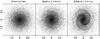 |
Fig. 6 Gaseous disk from three models with different holes at time 0.5 Gyr. From left to right: spherical halo, tri-axial halo with a:b:c = 1:0.8:0.6, and tri-axial halo with a:b:c = 1:0.6:0.4. These models are similar to the one described in Sect. 3.5. |
4. Conclusions
In this paper we successfully applied the iterative method presented in our previous article (RAS09) to a particularly difficult problem, namely the construction of equilibrium initial conditions for simulations of disk galaxies including a gaseous component and/or a triaxial halo. Our iterative method relies on constrained (or guided) evolution, and is both simple and powerful. In our previous article we presented an algorithm for constructing an axisymmetric multicomponent model of a disk galaxy. Here we extended the application to models with gaseous components and models with non-axisymmetric haloes. We thus developed an algorithm for constructing an equilibrium gaseous disk in the presence of an axisymmetric or non-axisymmetric external potential. We tested our method for two types of gas. The first type is isothermal gas, and the second type is a sub-resolution multiphase model for star-forming gas, developed by Springel & Hernquist (2003). We also presented an algorithm for constructing a stellar disk embedded in a non-axisymmetric external potential.
We discussed two test models of disk galaxies. The first model consists of a spherical halo, a stellar disk, and an isothermal gaseous disk. The second model consists of a triaxial halo, a stellar disk, and a star-forming gaseous disk. We demonstrated that both models are very close to equilibrium. In all cases, we gave sufficient explanations to allow the reader to reproduce the algorithm in his/her own code.
Although algorithms for creating isolated triaxial systems (e.g. for elliptical galaxy models) have already been presented elsewhere (Schwarzschild 1979; Rodionov et al. 2009; Dehnen 2009), this is, to our knowledge, the first proposed algorithm for a multicomponent disk galaxy system, with a triaxial halo and non-axisymmetric gaseous and stellar disks. Thus this work paves the way to many studies of realistic galaxy disks and the formation and evolution of their structures and substructures.
Acknowledgments
We thank V. Springel for the use of a non-public version of his GADGET2 code, which includes sub-grid physics and the referee, C. Struck, for a constructive report. This work was partially supported by grant ANR-06-BLAN-0172, by the Russian Foundation for Basic Research (grants 08-02-00361-a and 09-02-00968-a) and by a grant from the President of the Russian Federation for support of Leading Scientific Schools (grant NSh-1318.2008.2).
References
- Dehnen, W. 2000, ApJ, 536, 39 [Google Scholar]
- Dehnen, W. 2002, J. Comput. Phys., 179, 27 [Google Scholar]
- Dehnen, W. 2009, MNRAS, 395, 1079 [NASA ADS] [CrossRef] [MathSciNet] [Google Scholar]
- Hernquist, L. 1993, ApJS, 86, 389 [NASA ADS] [CrossRef] [Google Scholar]
- Kenney, J. F., & Keeping, E. S. 1951, Mathematics of Statistics, Pt. 2, 2nd edn. (Princeton, NJ: Van Nostrand) [Google Scholar]
- Kennicutt, R. C. 1998, ApJ, 498, 541 [NASA ADS] [CrossRef] [Google Scholar]
- Machado, R. E. G., & Athanassoula, E. 2010, MNRAS, 406, 2386 [NASA ADS] [CrossRef] [Google Scholar]
- Navarro, J. F., Frenk, C. S., & White, S. D. M. 1996, ApJ, 462, 563 [NASA ADS] [CrossRef] [Google Scholar]
- Rodionov, S. A., Athanassoula, E., & Sotnikova, N. Ya. 2009, MNRAS, 392, 904 (RAS09) [NASA ADS] [CrossRef] [Google Scholar]
- Schwarzschild, M. 1979, ApJ, 232, 236 [NASA ADS] [CrossRef] [Google Scholar]
- Sotnikova, N. Ya., & Rodionov, S. A. 2006, Astron. Lett., 32, 649 [NASA ADS] [CrossRef] [Google Scholar]
- Springel, V. 2005, MNRAS, 364, 1105 [NASA ADS] [CrossRef] [Google Scholar]
- Springel, V., & Hernquist, L. 2003, MNRAS, 339, 289 [Google Scholar]
- Springel, V., Di Matteo, T., & Hernquist, L. 2005, MNRAS, 361, 776 [NASA ADS] [CrossRef] [Google Scholar]
Appendix A: Checking the convergence
In simulation projects on galaxies it is customary to run a relatively large number of simulations to inter-compare and understand the effect of various parameters. Thus, creating the initial conditions can be a considerable part of the work and it makes sense to streamline it. In particular, the amount of CPU involved depends on the number of iteration steps made. This number should be sufficiently large, so that the iteration procedure can converge, but not excessively large, so as not to needlessly waste time. It is thus necessary to be able to assess whether the iteration has converged or not. The most straightforward way is of course to plot the evolution in time of various radial profiles (such as the density, the mean velocities and dispersions etc.) and check by eye whether the variation between the two last iteration times is sufficiently small. This, however, can be very tedious, particularly if it is carried out a number of times for each initial conditions. It is thus useful to prepare tools that can give information on whether a rough convergence has been achieved, before starting the visual examination. In this appendix we will describe how this can be carried out in practice. We aim to compare the system in the beginning and in the end of a short-term evolution during a single iterative step. So we need tools to compare two N-body models (in this context, a gaseous disk consisting of SPH particles can also be considered as an N-body model). We note that the following algorithm is fairly similar to a test of the statistical hypothesis that two N-body systems are just two random realizations of the same distribution function (hereafter DF). Our algorithm is based on comparisons of profiles of different quantities.
We wish to compare profiles of some quantity Q along some axis A for both systems. We divide these systems into pieces along the axis A in a way that each piece contains approximately the same number of particles. For this, we divide the first system into pieces, each containing the same number of particles and calculate the corresponding boundaries of these pieces in the first system. We then divide the second system by means of these boundaries. In each piece we calculate a given quantity whose value we denonte by Q. Let q1,i, q2,i be the calculated values in the ith piece in the first and the second model, respectively. If we consider the N-body system as a random realization of some DF, then each value calculated in this system can be considered as a random variable. Let Qi be random variable defined as the value Q calculated in piece i. For example, if the two systems under consideration are just two random realization of the same DF, then q1,i and q2,i are two samples of the random variable Qi. We can estimate the variance of this random variable. Let var1,i and var2,i be estimates of the variance of Qi calculated for the first and the second system, respectively, and let us consider the value 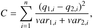 (A.1)where n is the total number of pieces. If the distribution of Qi is close to a normal distribution and var1,i and var2,i are close to the real variance, then the distribution of C should be close to a chi-square distribution with n degrees of freedom
  (Kenney & Keeping 1951). Such a distribution has a mean equal to n and a variance equal to 2 n. According to the central limit theorem, as n tends to infinity, the tends to normal distribution. So in a first approximation the values of
  (A.2)have a distribution close to the normal distribution with mean equal to 0 and variance equal to 1. Consequently, if value H ≲ 3, then the value of C can be explained by the fact that the number of particles is finite, even in the case when the two N-body systems under consideration are just two random realizations of the same DF. Otherwise, if H ≳ 3, then these N-body systems probably differ, because the value of C can be hardly explained by the fact that the number of particles is finite. In other words, the value of H gives us the distance between the two profiles of the quantity Q (calculated for the two different N-body systems) measured in sigmas.
We use three types of quantities Q: the number of particles in the piece, the mean of some quantity, and the dispersion of some quantity. We need to estimate the variance of the random variable Qi in these cases. Let us choose some parameter of the particles f. If Q is the mean of the values of f, then the variance of the random variable Qi (the variance of the sample mean) can be estimated as  (A.3)where
  is the variance of the quantity f and ni is the number of particles in piece i. If Q is the variance of the values of f then
the variance of random variable Qi (this is the variance of sample variance) can be calculated as  (A.4)where
  and m4 are the second and fourth central moments of variable f in piece i (Kenney & Keeping 1951, p. 164). And in the last case then Q is the number of particles in piece i. For a fixed division of the system the random variable Qi has a binomial distribution. And if ni ≪ N, where N is total number of particles, the variance of Qi can be estimated as varn = ni. But we note that in our case the situation is more complicated because our algorithm of division of the systems. But we assume that this formula is valid in our case, more precisely, we assume that in Eq. (A.1) var1,i + var2,i = n1,i + n2,i.
To check the convergence of the iteration in terms of some value Q, we calculate the value of H for the last 10 iterations. If the mean of these ten values H10 is less than 3, then it means that profile of Q does not change at all during one iteration. It is a very strict criterion, and for practical purposes we assume that iteration has converged if H10 is less than 10.
All Figures
|
Fig. 1 General scheme of the iterative method. |
| In the text | |
|
Fig. 2 Initial evolutionary stages for the gaseous disk of the constructed disk galaxy model (axisymmetric isothermal case). The evolution of the model was calculated including a live halo and stellar disk. The upper snapshots show the disk views face-on for times 0, 0.1, 0.2, 0.3 and 0.4; the grey intensities correspond to the logarithm of the surface density. The bottom panels show the dependence of various disk quantities on the cylindrical radius R at the same times. Here Σg is the surface density of the gas; z1/2 is the median of the |z| value, i.e a measure of the disk thickness (see Sotnikova & Rodionov 2006) and |
| In the text | |
|
Fig. 3 Initial evolutionary stages for the gaseous disk of the constructed disk galaxy model (with triaxial halo and star-forming gas). We show the same quantities as in Fig. 2, except for the bottom right panel, which shows the dependence of the mean thermal energy on R. |
| In the text | |
|
Fig. 4 Initial evolutionary stages for the stellar disk of the constructed disk galaxy model (with triaxial halo and star-forming gas). The upper snapshots show the disk viewed face-on for times 0, 0.1, 0.2, 0.3 and 0.4; the grey intensities correspond to the logarithms of particle number density. The bottom panels show the dependence of various disk quantities on the cylindrical radius R at the same times. Here n is the number of particles in concentric cylindrical layers; z1/2 is the median of the value |z|, and σR is the radial velocity dispersion. |
| In the text | |
|
Fig. 5 Initial evolutionary stages for the halo of the constructed disk galaxy model (with triaxial halo and star-forming gas). We show the dependence of various quantities on the spherical radius r for various moments of time, a) shows radial profiles of axial ratios b/a and c/a. These profiles were calculated by means of the method described in Machado & Athanassoula (2010); b) shows the profile of the number of particles n in concentric spherical layers; c) shows the profile of the radial velocity dispersion. |
| In the text | |
|
Fig. 6 Gaseous disk from three models with different holes at time 0.5 Gyr. From left to right: spherical halo, tri-axial halo with a:b:c = 1:0.8:0.6, and tri-axial halo with a:b:c = 1:0.6:0.4. These models are similar to the one described in Sect. 3.5. |
| In the text | |
Current usage metrics show cumulative count of Article Views (full-text article views including HTML views, PDF and ePub downloads, according to the available data) and Abstracts Views on Vision4Press platform.
Data correspond to usage on the plateform after 2015. The current usage metrics is available 48-96 hours after online publication and is updated daily on week days.
Initial download of the metrics may take a while.