| Issue |
A&A
Volume 529, May 2011
|
|
|---|---|---|
| Article Number | A127 | |
| Number of page(s) | 5 | |
| Section | The Sun | |
| DOI | https://doi.org/10.1051/0004-6361/201016320 | |
| Published online | 15 April 2011 | |
Chromospheric velocities of a C-class flare⋆
Astrophysics Research Centre, School of Mathematics and Physics, Queen’s University, Belfast BT7 1NN, Northern Ireland, UK
e-mail: This email address is being protected from spambots. You need JavaScript enabled to view it.
Received: 14 December 2010
Accepted: 10 March 2011
Abstract
Aims. We use high spatial and temporal resolution observations from the Swedish Solar Telescope to study the chromospheric velocities of a C-class flare originating from active region NOAA 10969.
Methods. A time-distance analysis is employed to estimate directional velocity components in Hα and Ca ii K image sequences. Also, imaging spectroscopy has allowed us to determine flare-induced line-of-sight velocities. A wavelet analysis is used to analyse the periodic nature of associated flare bursts.
Results. Time-distance analysis reveals velocities as high as 64 km s-1 along the flare ribbon and 15 km s-1 perpendicular to it. The velocities are very similar in both the Hα and Ca ii K time series. Line-of-sight Hα velocities are red-shifted with values up to 17 km s-1. The high spatial and temporal resolution of the observations have allowed us to detect velocities significantly higher than those found in earlier studies. Flare bursts with a periodicity of ≈60 s are also detected. These bursts are similar to the quasi-periodic oscillations observed at hard X-ray and radio wavelength data.
Conclusions. Some of the highest velocities detected in the solar atmosphere are presented. Line-of-sight velocity maps show considerable mixing of both the magnitude and direction of velocities along the flare path. A change in direction of the velocities at the flare kernel has also been detected which may be a signature of chromospheric evaporation.
Key words: Sun: activity / Sun: chromosphere / Sun: flares
Movies associated to Fig. 5 are only available in electronic form at http://www.aanda.org
© ESO, 2011
1. Introduction
A flare is the result of magnetic field reconfiguration/annihilation, a process usually occurring in the corona (Parker 1963). Solar flares are highly energetic events with complex structures and properties, which transfer energy between various regions in the solar atmosphere. White-light flares (WLFs) exhibit strong emission in the white-light continuum, and are usually present in the most energetic of events, such as X- and M-class flares (Neidig & Cliver 1983). However, with the increasing use of space-based telescopes and ground-based observatories with high spatial resolutions, flares as low as C-class have been shown to demonstrate optical continuum enhancements (Matthews et al. 2003; Hudson et al. 2006). Jess et al. (2008) have recently suggested that all flares exhibit a degree of continuum enhancement, but that most observations will not have sufficient spatial or temporal resolution to capture this phenomena. The processes which ultimately lead to WL enhancements are still under review (Fletcher et al. 2007), particularly in the regime of small flare classifications.
Aschwanden et al. (2007) have suggested that the principal source of coronal heating during flare events may be in the transition region and the upper chromosphere. After the reconnection of magnetic field lines has occurred, the lower solar atmosphere is heated by either chromospheric evaporation or radiative back-warming. It is believed that the process which governs the heating of the lower solar atmosphere is determined by the magnitude of the flaring event. There have been flare models which explain two types of chromospheric evaporation: gentle evaporation (Antiochos & Sturrock 1978; Mariska et al. 1989) and explosive evaporation (Fisher et al. 1985; Milligan et al. 2006a,b). Gentle evaporation refers to a situation where the chromosphere is heated directly by non-thermal electrons, or heated indirectly by thermal conduction processes throughout the solar atmosphere. The chromospheric plasma will then lose energy through radiative processes and low-velocity hydrodynamic expansion. With explosive evaporation, the chromosphere is unable to radiate energy at a sufficiently high rate, resulting in the plasma expanding into the flaring loops at high velocities.
The other proposed heating mechanism is radiative back-warming (Machado et al. 1989). Under this regime, electron beams bombard the chromosphere after magnetic reconnection occurs in the corona. However, most of the electrons will not have sufficient energy to pass through the dense chromospheric plasma, and so will not reach the photosphere. On the other hand, physical conditions linking the chromosphere and photosphere will promote the movement of energy towards the photosphere; hence the term back-warming. This process is not as impulsive as chromospheric evaporation, and may help explain the origin of WL emission seen in low energy events.
The present paper uses high temporal, spatial and spectral resolution observations to study the chromospheric velocities of a C-class flare. In Sect. 2 we discuss the observations and image reconstruction techniques employed, while Sect. 3 describes the analysis methods employed on the dataset and presents our results. Concluding remarks are given in Sect. 4.
2. Observations
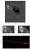 |
Fig. 1 a) A snapshot of the full 68′′ × 68′′ field-of-view captured through the Hα wideband filter. An expanded view of the flare region in Hαb) and Ca ii K core c) are also shown with sample positions for the time-distance slice method used in Sects. 3.1 and 3.2. A box is included in both image b) and c) to highlight one of the brightenings used to determine the horizontal bulk plasma velocities summarised in Table 1. A sample time-distance plot using the slice position indicated in c) is shown also d). The blue line shows the gradient used to establish the velocity. |
Data presented here are part of an observing sequence obtained on 2007 August 24, with the Swedish Solar Telescope (SST) on the island of La Palma. The optical setup allowed us to image a 68″ × 68″ region surrounding active region NOAA 10969, complete with solar rotation tracking. This active region was located at heliocentric co-ordinates (−516″, −179″), or S05E33 in the solar NS-EW co-ordinate system. The Solar Optical Universal Polarimeter (SOUP) was implemented to provide two-dimensional spectral information across the Hα line profile centred at 6562.8 Å, which was sampled using 7 wavelength positions followed by a Gaussian fit to the line profile. Doppler velocities were established using the methods detailed in Suematsu et al. (1995) and a Doppler map, Dopp = (Cb − Cr) / (Cb + Cr + 2), was constructed. In this equation, Cb and Cr are contrast images obtained using the relation C = (I − Ia) / Ia where Ia corresponds to the average intensity over the entire dataset, while the subscripts b and r correspond to the wavelengths at Hα-core − 700 mÅ and Hα-core + 700 mÅ, respectively. A second camera provided simultaneous wideband images centered with a FWHM of 8 Å centered in Hα (Langangen et al. 2008).
In addition, a series of Ca ii interference filters were used to provide high-cadence imaging in this portion of the optical spectrum. A filter centred at 3953.7 Å with a band width of 10 Å was employed to acquire data in the Ca ii K/H continuum whilst a 1.5 Å filter band centred at 3934.2 Å was used to acquire data in Ca ii K.
The observations employed in the present analysis consist of 39000 images at each wavelength, taken with a 0.12 s cadence, providing just over one hour of uninterrupted data. Our Hα images have a sampling of 0.068″ per pixel, to match the telescope’s diffraction-limited resolution to that of the 1024 × 1024 pixel2 CCD. Images of the Ca ii K core were captured using a 2048 × 2048 pixel2 CCD with a sampling of 0.034″ per pixel. Although the Ca ii K camera was oversampled, this was deemed necessary to keep the dimensions of the field-of-view the same for both cameras. A high order adaptive optics system that corrects for approximately 35 Karhunen-Loeve modes was utilized throughout the data acquisition (Scharmer et al. 2003). The acquisition time for this observing sequence was early in the morning, and seeing conditions were excellent with minimal variation throughout the time series. During the observing sequence a C2.0 flare was observed, originating from NOAA 10969 at 07:49 UT.
Multi-object multi-frame blind deconvolution (MOMFBD; van Noort et al. 2005) image restoration was implemented to remove small-scale atmospheric distortions present in both data sets. Sets of 80 exposures were included in the restorations, producing a new effective cadence of 9 s for the Hα observations. The Ca ii K core data incorporated 20 exposures in each restoration, producing a new effective cadence of 2.5 s. All reconstructed images were subjected to a Fourier co-aligning routine, in which cross-correlation and squared mean absolute deviation techniques are utilized to provide sub-pixel co-alignment accuracy. The full field-of-view with expanded versions of the flare is shown in Fig. 1. Movies of the event as seen in the Hα wideband and Ca ii K core spectral lines have been included as an on-line resource material to emphasise the high temporal and spatial resolution of this dynamic event (see Fig. 5).
3. Results and discussion
3.1. Flare velocities
The horizontal velocity components in the Hα wideband and Ca ii K core images are investigated using time-distance analysis. We place a one-dimensional slice through each of the data sets to generate intensity maps as a function of distance and time.
The slice was initially positioned at the flare kernel (Jess et al. 2008), and extended along the flare ribbon, allowing accurate velocity measurements as a function of distance from this reference point (Fig. 1c). Errors are evaluated by fitting the data with a least squares fit. The temporal evolution of the chromospheric velocities for Ca ii K and Hα, determined using the slice method, are shown in Fig. 2. Velocities peak at a value of 64 ± 11 km s-1 in both wavelengths, and then these are reached ≈ 90 s after the Ca ii K intensity peak. To minimize the effects of small-scale fluctuations along the flare ribbon, we have also determined the velocities using a wider slice of 15 pixels, revealing identical results. The velocities found are within the error bars of those determined with a narrow slice, suggesting the plasma flows uniformly along a direct path towards the flare kernel. Bulk plasma velocities are also calculated by tracking individual flare brightenings in the Hα data and the Ca ii K core images. Table 1 summarizes the velocities of three brightenings, with one such brightening enclosed in a box in Figs. 1b, c. We find these bulk motions do not follow the general movement of the flare ribbon, but instead they move independently across the top of the flare structure.
Velocity components perpendicular to the flare ribbon are also estimated using a similar approach. This form of analysis is employed on the Ca ii K datacube, as its superior temporal resolution allows small-scale velocities to be disentangled with a high degree of precision. An average velocity of 15.5 ± 0.6 km s-1 is found perpendicular to the flare ribbon, with velocities directed towards the flare ribbon.
Velocities of bright points.
The spectroscopic information provided by the SOUP instrument allows us to derive the line-of-sight (LOS) Doppler velocity components of the flare ribbon with an effective cadence of 63 s (Jess et al. 2010). In Fig. 3 we show the velocity maps derived from the Hα scans. The average LOS velocity in the immediate viscinity of flare-induced brightenings was found to be 14.83 ± 0.29 km s-1, peaking at 22.5 km s-1. Further examination of the Doppler maps reveals a shift in velocity direction at the location of the flare kernel between the first and second scans. The first frame exhibits a red-shifted velocity of 6.06 ± 0.28 km s-1, while the subsequent frame shows a blue-shifted velocity of 14.8 ± 0.3 km s-1 at the same position. It is possible that this shift from a red-shifted to a blue-shifted velocity is a signature of a chromospheric evaporation process, whereby accelerated electrons/plasma strike the lower solar atmosphere, resulting in material being ejected into the flaring loops. Figure 3 also highlights considerable mixing of both the magnitude and direction of flare-induced velocities over the entire flare ribbon.
Velocities of 54.5 ± 2.3 km s-1 and 52.8 ± 2.5 km s-1 for the Hα and Ca ii K core datacubes, respectively, show that velocities along the flare ribbon are very similar in these chromospheric lines. Utilizing a wider slit, followed by coarse spatial averaging, produced velocities of 58.1 ± 2.2 km s-1 and 59.0 ± 1.8 km s-1 for the Hα wideband and Ca ii K core images, respectively. Again, these values reiterate flare-induced velocities that are consistent along a direct path towards the flare kernel. We emphasize that, given the broad nature of the Hα line profile, the velocities determined from the Hα wideband are chromospheric.
Falchi et al. (2006) examined the Ca ii K spectral line of a C1.0 flare and found LOS velocities of 10–20 km s-1, with He i and O v observations indicating velocities closer to 40 km s-1. During the same observing campaign, Teriaca et al. (2006) report on a larger C2.3 class flare which occurred within the same active region, with He i and O v velocities of ≈20 km s-1. The velocities presented here are substatially larger than previously published results for C-class flares.
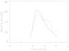 |
Fig. 2 The evolution of flare velocities in Hα (solid red line) and Ca ii K core (dot-dashed blue line) images, determined using a slice along the flare ribbon. The data sequence begins at 07:50:34 UT. |
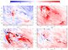 |
Fig. 3 Line-of-sight velocities of the flare region determined from the Hα SOUP scans; a)–d) are velocity maps obtained at 07:50:40 UT, 07:51:23 UT, 07:52:26 UT and 07:53:29 UT respectively. The colour scale represents line-core Doppler shifts and is displayed in km s-1. |
Moving on to more energetic events, Maurya & Ambastha (2009) observed transient features associated with X17 and X10 WLFs and derived photospheric and chromospheric velocities of 30–50 km s-1. Furthermore, work by Milligan et al. (2006a) found X-class flare-induced downflows of 36 ± 16 km s-1 at chromospheric temperatures. The values established for the presented Ca ii K core data, in particular, show remarkable agreement with the chromospheric velocity results determined by Maurya & Ambastha (2009), albeit originating from a much lower energy event.
We believe that the higher velocities established here for less-energetic events are a direct result of the superior spatial and temporal resolution offered by the SST, which can be clearly seen in the movies provided as an on-line resource (see Fig. 5). Indeed, the velocities uncovered here are consistent with current radiative hydrodynamic simulations of solar flares, where Allred et al. (2005) determine the response of the solar atmosphere to a beam of non-thermal electrons, injected at the apex of a closed coronal loop. The results of their simulations for typical M- and X-class flares produce velocities of ~ 40 km s-1 in the lower chromosphere. Thus, the velocities presented here demonstrate a striking resemblence to current theoretical models of solar flares.
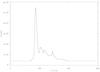 |
Fig. 4 A sample light curve of the flaring event generated by methods discussed in Sect. 3.2. This light curve clearly demonstrates the periodic nature of the flare bursts. The average period of the flare bursts was ≈60 s, and all values were found to be well above the 3σ confidence level. |
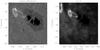 |
Fig. 5 Stills from the two movies illustrating the temporal and spatial evolution of a C2.0 class flare observed on 2007 August 24 in active region NOAA 10969 with the Swedish Solar Telescope. The data have been obtained with a wide band filter centered in Hα (FWHM 8 Å) and a filter centered in the Ca ii K core (FWHM 1.5 Å). This flare has shown a white-light continuum previously reported by Jess et al. (2008). The first frame in the Ca K movie was obtained at 07:50:30 UT and the corresponding frame in the Hα wideband was acquired at 07:50:40 UT. Imaging spectroscopy of the event revealed high chromospheric velocities and quasi-periodic oscillations similar to those detected in hard X-ray and radio wavelengths. The results and methodology are discussed in detail in the text. Movies are available online. |
3.2. Periodic variations
Analysis of the lightcurve associated with the flare revealed 4 periodic bursts (Fig. 4) with an average periodicity of ≈ 60 s. The period was determined using wavelet analysis (Torrence & Compo 1998). Bursts were found to exist at a distance of ≈ 30 Mm from the flare kernel, in a region encompassing the main loop structure of the flare (Fig. 1). A control test was performed over a quiet region of the data set using the same technique employed on the flare region. The outcome of this test confirmed that the intensity fluctuations were not the result of variations in seeing conditions.
Periodic flare brightnenings are often interpreted in terms of quasi-periodic pulsations (QPPs) (Nakariakov & Melnikov 2009). QPP studies (Nakariakov et al. 2010) have found periods of 40 s in gamma-ray, hard X-ray and microwave emissions. Therefore, it is possible that the 40–80 s oscillations found in optical emissions within this study are a result of flare-induced QPPs. Additionally, work by McAteer et al. (2005) found periods between 40–80 s along the ribbon of a C9.6 class flare. Flare-induced acoustic waves in the overlying coronal loops were thought to be responsible for the periodic brightenings in this study. Although the periodic bursts presented here are observed away from the flare kernel, the fact that the observed periods agree with the study of McAteer et al. (2005) suggests these oscillations extend beyond the boundaries of the magnetic flux tube and into the chromosphere.
4. Conclusions
We have utilized high spatial and temporal resolution imaging, and imaging spectroscopy of the lower solar atmosphere to derive velocities associated with a relatively low energy C-class flare. Velocities across the solar surface have values as high 64 km s-1, while line-of-sight (LOS) velocities show both redshifts and blueshifts up to 17 km s-1. These are some of the highest velocities detected in the lower solar atmosphere. Bulk plasma motions were observed to move across the flare ribbon at velocities as high as 55 km s-1, seemingly independent of the general flare ribbon motion. A time-distance slice employed parallel to the flare ribbon found velocities as high as 64 km s-1 for Hα wideband data and as high as 59 km s-1 for Ca ii K core data. Varying spatial averages of the time-distance slice produced similar values, indicating a uniform motion on large spatial scales. Analysis of the LOS components of the flare found velocities as high as 17 km s-1, with substantial mixing of both magnitude and direction of flare-induced velocities. Also, a velocity direction change at the flare kernel was observed in the LOS Doppler maps, which could be attributed to a form of chromospheric evaporation. Examination of the light curve associated with the flare event displays a periodic nature, whereby bursts are emitted at ≈ 60 s intervals. In addition, a comparison with more energetic flares indicate that flare-induced velocities are not necessarily directly related with the magnitude of the event.
Online material
Movies associated to Fig. 5
Movie 1
Access Supplementary Material
Movie 2
Access Supplementary MaterialAcknowledgments
P.H.K. thanks the Northern Ireland Department for Employment and Learning for a Ph.D. studentship. D.B.J. thanks the Science and Technology Facilities Council for a Post-Doctoral Fellowship. F.P.K. is grateful to AWE Aldermaston for the award of a William Penney Fellowship. The Swedish 1-m Solar Telescope is operated on the island of La Palma by the Institute for Solar Physics of the Royal Swedish Academy of Sciences in the Spanish Observatorio del Roque de los Muchachos of the Instituto de Astrofísica de Canarias. These observations have been funded by the Optical Infrared Coordination network (OPTICON), a major international collaboration supported by the Research Infrastructures Programme of the European Commissions Sixth Framework Programme.
References
- Allred, J. C., Hawley, S. L., Abbett, W. P., & Carlsson, M. 2005, ApJ, 630, 573 [NASA ADS] [CrossRef] [Google Scholar]
- Antiochos, S. K., & Sturrock, P. A. 1978, ApJ, 220, 1137 [NASA ADS] [CrossRef] [Google Scholar]
- Aschwanden, M. J., Winebarger, A., Tsiklauri, D., & Peter, H. 2007, ApJ, 659, 1673 [NASA ADS] [CrossRef] [Google Scholar]
- Falchi, A., Teriaca, L., & Maltagliati, L. 2006, Sol. Phys., 239, 193 [NASA ADS] [CrossRef] [Google Scholar]
- Fisher, G. H., Canfield, R. C., & McClymont, A. N. 1985, ApJ, 289, 414 [NASA ADS] [CrossRef] [Google Scholar]
- Fletcher, L., Hannah, I. G., Hudson, H. S., & Metcalf, T. R. 2007, ApJ, 656, 1187 [NASA ADS] [CrossRef] [Google Scholar]
- Hudson, H. S., Wolfson, C. J., & Metcalf, T. R. 2006, Sol. Phys., 234, 79 [NASA ADS] [CrossRef] [Google Scholar]
- Jess, D. B., Mathioudakis, M., Crockett, P. J., & Keenan, F. P. 2008, ApJ, 688, L119 [NASA ADS] [CrossRef] [Google Scholar]
- Jess, D. B., Mathioudakis, M., Browning, P. K., Crockett, P. J., & Keenan, F. P. 2010, ApJ, 712, L111 [NASA ADS] [CrossRef] [Google Scholar]
- Langangen, Ø., Rouppe van der Voort, L., & Lin, Y. 2008, ApJ, 673, 1201 [NASA ADS] [CrossRef] [Google Scholar]
- Machado, M. E., Emslie, A. G., & Avrett, E. H. 1989, Sol. Phys., 124, 303 [NASA ADS] [CrossRef] [Google Scholar]
- Mariska, J. T., Emslie, A. G., & Li, P. 1989, ApJ, 341, 1067 [NASA ADS] [CrossRef] [Google Scholar]
- Matthews, S. A., van Driel-Geszteyli, L., Hudson, H. S., & Nitta, N. V. 2003, A&A, 409, 1107 [NASA ADS] [CrossRef] [EDP Sciences] [Google Scholar]
- Maurya, R. A., & Ambastha, A. 2009, Sol. Phys., 258, 31 [NASA ADS] [CrossRef] [Google Scholar]
- McAteer, R. T. J., Gallagher, P. T., Brown, D. S., et al. 2005, ApJ, 620, 1101 [NASA ADS] [CrossRef] [Google Scholar]
- Milligan, R. O., Gallagher, P. T., Mathioudakis, M., et al. 2006a, ApJ, 638, L117 [NASA ADS] [CrossRef] [Google Scholar]
- Milligan, R. O., Gallagher, P. T., Mathioudakis, M., & Keenan, F. P. 2006b, ApJ, 642, L169 [NASA ADS] [CrossRef] [Google Scholar]
- Nakariakov, V. M., & Melnikov, V. F. 2009, Space Sci. Rev., 55 [Google Scholar]
- Nakariakov, V. M., Foullon, C., Myagkova, I. N., & Inglis, A. R. 2010, ApJ, 708, L47 [NASA ADS] [CrossRef] [Google Scholar]
- Neidig, D. F., & Cliver, E. W. 1983, Sol. Phys., 88, 275 [NASA ADS] [CrossRef] [Google Scholar]
- Parker, E. N. 1963, ApJS, 8, 177 [NASA ADS] [CrossRef] [Google Scholar]
- Scharmer, G. B., Dettori, P. M., Lofdahl, M. G., & Shand, M. 2003, Proc. SPIE, 4853, 370 [Google Scholar]
- Suematsu, Y., Wang, H., & Zirin, H. 1995, ApJ, 450, 411 [NASA ADS] [CrossRef] [Google Scholar]
- Teriaca, L., Falchi, A., Falciani, R., Cauzzi, G., & Maltagliati, L. 2006, A&A, 455, 1123 [NASA ADS] [CrossRef] [EDP Sciences] [Google Scholar]
- Torrence, C., & Compo, G. P. 1998, Bull. Am. Meteorol. Soc., 79, 61 [Google Scholar]
- van Noort, M., Rouppe van der Voort, L., & Löfdahl, M. G. 2005, Sol. Phys., 228, 191 [NASA ADS] [CrossRef] [Google Scholar]
All Tables
All Figures
|
Fig. 1 a) A snapshot of the full 68′′ × 68′′ field-of-view captured through the Hα wideband filter. An expanded view of the flare region in Hαb) and Ca ii K core c) are also shown with sample positions for the time-distance slice method used in Sects. 3.1 and 3.2. A box is included in both image b) and c) to highlight one of the brightenings used to determine the horizontal bulk plasma velocities summarised in Table 1. A sample time-distance plot using the slice position indicated in c) is shown also d). The blue line shows the gradient used to establish the velocity. |
| In the text | |
|
Fig. 2 The evolution of flare velocities in Hα (solid red line) and Ca ii K core (dot-dashed blue line) images, determined using a slice along the flare ribbon. The data sequence begins at 07:50:34 UT. |
| In the text | |
|
Fig. 3 Line-of-sight velocities of the flare region determined from the Hα SOUP scans; a)–d) are velocity maps obtained at 07:50:40 UT, 07:51:23 UT, 07:52:26 UT and 07:53:29 UT respectively. The colour scale represents line-core Doppler shifts and is displayed in km s-1. |
| In the text | |
|
Fig. 4 A sample light curve of the flaring event generated by methods discussed in Sect. 3.2. This light curve clearly demonstrates the periodic nature of the flare bursts. The average period of the flare bursts was ≈60 s, and all values were found to be well above the 3σ confidence level. |
| In the text | |
|
Fig. 5 Stills from the two movies illustrating the temporal and spatial evolution of a C2.0 class flare observed on 2007 August 24 in active region NOAA 10969 with the Swedish Solar Telescope. The data have been obtained with a wide band filter centered in Hα (FWHM 8 Å) and a filter centered in the Ca ii K core (FWHM 1.5 Å). This flare has shown a white-light continuum previously reported by Jess et al. (2008). The first frame in the Ca K movie was obtained at 07:50:30 UT and the corresponding frame in the Hα wideband was acquired at 07:50:40 UT. Imaging spectroscopy of the event revealed high chromospheric velocities and quasi-periodic oscillations similar to those detected in hard X-ray and radio wavelengths. The results and methodology are discussed in detail in the text. Movies are available online. |
| In the text | |
Current usage metrics show cumulative count of Article Views (full-text article views including HTML views, PDF and ePub downloads, according to the available data) and Abstracts Views on Vision4Press platform.
Data correspond to usage on the plateform after 2015. The current usage metrics is available 48-96 hours after online publication and is updated daily on week days.
Initial download of the metrics may take a while.