| Issue |
A&A
Volume 529, May 2011
|
|
|---|---|---|
| Article Number | A101 | |
| Number of page(s) | 13 | |
| Section | The Sun | |
| DOI | https://doi.org/10.1051/0004-6361/201015569 | |
| Published online | 12 April 2011 | |
Simulating flaring events in complex active regions driven by observed magnetograms
1
University of AthensDepartment of Physics, 15483 Athens, Greece
e-mail: This email address is being protected from spambots. You need JavaScript enabled to view it.
2
University of Thessaloniki, Department of Physics, 54006 Thessaloniki, Greece
3
Research Center of Astronomy and Applied Mathematics, Academy of Athens, 11527, Greece
Received: 11 August 2010
Accepted: 8 February 2011
Abstract
Context. We interpret solar flares as events originating in active regions that have reached the self organized critical state, by using a refined cellular automaton model with initial conditions derived from observations.
Aims. We investigate whether the system, with its imposed physical elements, reaches a self organized critical state and whether well-known statistical properties of flares, such as scaling laws observed in the distribution functions of characteristic parameters, are reproduced after this state has been reached.
Methods. To investigate whether the distribution functions of total energy, peak energy and event duration follow the expected scaling laws, we first applied a nonlinear force-free extrapolation that reconstructs the three-dimensional magnetic fields from two-dimensional vector magnetograms. We then locate magnetic discontinuities exceeding a threshold in the Laplacian of the magnetic field. These discontinuities are relaxed in local diffusion events, implemented in the form of cellular automaton evolution rules. Subsequent loading and relaxation steps lead the system to self organized criticality, after which the statistical properties of the simulated events are examined. Physical requirements, such as the divergence-free condition for the magnetic field vector, are approximately imposed on all elements of the model.
Results. Our results show that self organized criticality is indeed reached when applying specific loading and relaxation rules. Power-law indices obtained from the distribution functions of the modeled flaring events are in good agreement with observations. Single power laws (peak and total flare energy) are obtained, as are power laws with exponential cutoff and double power laws (flare duration). The results are also compared with observational X-ray data from the GOES satellite for our active-region sample.
Conclusions. We conclude that well-known statistical properties of flares are reproduced after the system has reached self organized criticality. A significant enhancement of our refined cellular automaton model is that it commences the simulation from observed vector magnetograms, thus facilitating energy calculation in physical units. The model described in this study remains consistent with fundamental physical requirements, and imposes physically meaningful driving and redistribution rules.
Key words: Sun: corona / Sun: flares / Sun: photosphere
© ESO, 2011
1. Introduction
Solar flares are transient energy release events above solar active regions (ARs). Populations of flares are known to exhibit robust statistical properties, which have been repeatedly identified in numerous observations. In particular, specific flare parameters have been consistently found to follow robust power laws with indices lying in well-defined ranges. More specifically, a series of flare observations (Datlowe et al. 1974; Lin et al. 1984; Sturrock et al. 1984; Dennis 1985; Vilmer 1987; Crosby et al. 1993; Biesecker 1994; Bromund et al. 1995; Polygiannakis et al. 2002) report that the distribution functions of peak flux, total energy, and event duration exhibit well-formed scaling laws with exponents in the ranges of (−1.59, −1.80), (−1.39, −1.50), and (−2.25, −2.80), respectively.
This consistency of the power-law indices identified in numerous independent studies stimulated a new phenomenological approach in reproducing and modeling the statistical behavior of flaring activity. Lu & Hamilton (1991) and Lu et al. (1993) were the first to construct a simple model of solar flare occurrence, based on the assumption that the solar corona is in a statistically stable self organized critical (SOC) state. In this context, ARs are perceived as nonlinear dissipative dynamical systems, externally driven by the photospheric velocity field. Localized instabilities are generated by random shuffling of the coronal loops’ footpoints in the photosphere and these instabilities are responsible for the fragmented energy release in the solar corona. The magnetic energy release simulated via cellular automaton (CA) modeling led to avalanche-like events. This model allows instabilities, simulating current sheet disruption and Ohmic dissipation, when a certain current density threshold is exceeded. An enhancement of the original SOC concept with respect to the instability criteria and the corresponding relaxation has been introduced by Vlahos et al. (1995) and Georgoulis et al. (1995). Both suggest that the initial instability may trigger secondary ones, thus affecting sites beyond the closest vicinity of the original event. Non-local treatment between flaring elements was also attempted by MacKinnon & Macpherson (1997). In addition, Georgoulis & Vlahos (1996) constructed a refined statistical flare model, including both isotropic and anisotropic relaxation mechanisms, as well as extended instability criteria.
This kind of modeling produced a double power-law scaling behavior: the flatter power law resembled intermediate and large flares, whereas the steeper one described low-energy events. An additional enhancement of this model lay in the external driver simulation. In the mentioned study, the driver of the system followed a power law itself, thus mimicking the instabilities triggered by the emerging magnetic flux from the convection zone in addition to photospheric shuffling. Further extensions were introduced by Georgoulis & Vlahos (1998), who presented a systematic study of the power law indices’ variability as a function of the driver’s properties. In this refined statistic flare model, Georgoulis & Vlahos attempted to model the stresses that are built up randomly within ARs through a highly variable, inhomogenous external driver. Although clearly deviating from the initial SOC models, the robust scaling laws in the flares’ distribution functions survived. Isliker et al. (2000; 2001) tried for the first time to associate the classical CA models’ components with physical variables. Magnetohydrodynamic (MHD) and CA approaches were connected through the physical interpretation of numerous CA elements, such as the grid variable, the time step, the spatial discreteness, the energy release process, and the role of diffusivity. This study revealed several inconsistencies in the CA modeling, such as the uncontrolled value of the magnetic field divergence (∇·B) and the nonavailability of secondary variables, such as the current density and the electric field. Such weaknesses were treated by the extended CA model (X-CA) introduced by Isliker et al. (2002).
In this study we present a model that adopts the Lu & Hamilton (1991) approach as the starting point and to which several enhancements are made towards a more physical CA model that integrates various aspects of observed ARs and flares: first and foremost, the initial boundary and initial conditions stem from observed vector magnetograms. This allows us to perform calculations in physical units, in direct comparison with observations (see for example the respective restrictions presented in Georgoulis et al. 2001). Time remains the only quantity expressed in arbitrary model units, as the photospheric vector magnetogram does not change during the simulation. An additional feature is that during the whole process (initial loading, relaxation of magnetic discontinuities and further driving) the requirement ∇·B ≃ 0 is explicitly imposed. For this purpose we have used a nonlinear force-free extrapolation method to generate the initial conditions from observed magnetograms and impose instability criteria related to actual physical processes. The magnetic field relaxation in the CA model follows the Lu & Hamilton (1991) principles. The driving process is also designed to obey specific rules that do not violate known physical processes in the corona.
The structure of this work is as follows. Section 2 describes the data used in this study along with the necessary corrections imposed on them. Section 3 explains in detail all the modules comprising our model: first the extrapolation technique (EXTRA), along with the discontinuities’ identification (DISCO) modules. Furthermore, the magnetic field relaxation module (RELAX) and finally the driving module (LOAD) are presented, which may trigger further instabilities in the simulated AR, following rules that mimic specific physical processes. Section 4 presents our results and discusses our findings. Finally, Sect. 5 summarizes our conclusions.
2. Dataset
Nonlinear force-free extrapolation techniques require vector magnetograms that are not as widely available as conventional line-of-sight magnetograms. Here we have created a database of 11 different AR vector magnetograms from the University of Hawaii Imaging Vector Magnetograph (IVM). IVM obtains Stokes images in photospheric lines with 7pm spectral resolution, 1.1 arcsec spatial resolution (~0.55 arcsec per pixel) over a field of 4.7 arcmin2 and polarimetric precision of 0.1% (Mickey et al. 1996). We used both fully-inverted and quick-look IVM data. Quick-look data were obtained from the IVM Survey Data archive (available online at http://www.cora.nwra.com/ivm/IVM-SurveyData). The quick-look data reduction differs from the complete inversion in that it uses a simplified flat-fielding approach, takes no account of scattered or parasitic light, and no correction is attempted for seeing variations that occur during the data acquisition.
In this study we used one fully inverted and ten quick-look IVM vector magnetograms. To remove the intrinsic azimuthal ambiguity of 180°, we used the Non-Potential magnetic Field Calculation (NPFC) method of Georgoulis (2005). For computational convenience we further rebinned the disambiguated magnetograms into a 32 × 32 regular grid.
3. The model
Our model consists of four separate modules. First we apply the Wiegelmann (2008) optimization algorithm to our vector magnetograms in order to nonlinearly extrapolate the magnetic field from the photospheric boundary (module “EXTRA”). We thus construct a three-dimensional (3d) 32 × 32 × 32 cube, within which the magnetic field is determined. Second, we identify the sites within our cubic grid that exceed a threshold in the magnetic field Laplacian (module “DISCO”). If unstable sites are found, we force the vicinity of the unstable location to undergo a magnetic-field restructuring. This redistribution is governed by specific rules, which do not violate basic physical laws. Under suitable conditions, the onset and relaxation of an initial instability may trigger a cascade of similar events in an avalanche-type manner. It is clear, therefore, that the wider vicinity, up to the entire system, may participate in this process. Module “RELAX” handles the field redistribution triggered by both the primary and subsequently triggered instabilities. The whole avalanche, comprised of a seed and the subsequently triggered instabilities, is considered as one single flare. After complete relaxation, we further drive the system via the “LOAD” module. There, a randomly selected grid site receives a random magnetic field increment.
3.1. “EXTRA”: a nonlinear force-free extrapolation module
The first step is to extrapolate the photospheric magnetic fields. As explained in Dimitropoulou et al. (2009), a physically meaningful treatment is the nonlinear force-free (NLFF) field extrapolation. Our method of choice is based on the optimization technique introduced by Wheatland et al. (2000) and further developed by Wiegelmann and collaborators (Wiegelmann 2004; Wiegelmann et al. 2006; Wiegelmann 2008). This technique reconstructs force-free magnetic fields from their boundary values by minimizing the Lorentz force and the divergence of the magnetic field vector in the extrapolation volume: ![Mathematical equation: \begin{equation} L=\int_{V}w(x,y,z)[|\vec{B}|^{-2}|(\vec{\nabla}\times\vec{B})\times\vec{B}|^{2}+|\nabla\cdot\vec{B}|^{2}]d^{3}x. \end{equation}](/articles/aa/full_html/2011/05/aa15569-10/aa15569-10-eq13.png) (1)In this functional, w(x,y,z) is a weighting function and V denotes the extrapolation volume. A force-free state is reached when L → 0 for w > 0. For w(x,y,z) = 1, the magnetic field must be available on all six boundaries of our cubic box for the optimization algorithm to work. However, photospheric vector magnetograms pertain only to the bottom boundary, whereas the magnetic field vector on the top and lateral boundaries is unknown. The weighting function is thus used to minimize the dependence of the interior solution from the unknown boundaries. In this study we introduce a buffer zone of ten grid points expanding to the lateral and top boundaries of the computational box. We then choose w(x,y,z) = 1 in the inner domain and let w drop to zero with a cosine-profile in the buffer zone towards the lateral and top boundaries of the computational box. This technique was first described by Wiegelmann (2004).
(1)In this functional, w(x,y,z) is a weighting function and V denotes the extrapolation volume. A force-free state is reached when L → 0 for w > 0. For w(x,y,z) = 1, the magnetic field must be available on all six boundaries of our cubic box for the optimization algorithm to work. However, photospheric vector magnetograms pertain only to the bottom boundary, whereas the magnetic field vector on the top and lateral boundaries is unknown. The weighting function is thus used to minimize the dependence of the interior solution from the unknown boundaries. In this study we introduce a buffer zone of ten grid points expanding to the lateral and top boundaries of the computational box. We then choose w(x,y,z) = 1 in the inner domain and let w drop to zero with a cosine-profile in the buffer zone towards the lateral and top boundaries of the computational box. This technique was first described by Wiegelmann (2004).
An additional useful attribute of Wiegelmann’s NLFF field extrapolation code is the preprocessing option it offers. As the photospheric magnetic field is in principle inconsistent with the force-free approximation, a preprocessing procedure was developed by Wiegelmann et al. (2006) in order to drive photospheric fields closer to an NLFF field equilibrium. Preprocessing minimizes the forces and torques in the system, thus satisfying the force-free requirements more closely.
Although NLFF extrapolation methods have been greatly improved in recent years, such models still include numerous uncertainties (DeRosa et al. 2009). Additional constraints stem from the measurements (signal-to-noise ratio, inadequate resolution of the 180° ambiguity) or from physical origins (variation in the line formation height, the non-force-free nature of the photospheric vector magnetograms), which are not adequately handled in the course of the extrapolation. Such uncertainties are unavoidably conveyed to our simulations.
3.2. “DISCO”: a module to identify magnetic-field instabilities
We assume that instabilities occur if the magnetic field stress exceeds a critical threshold. For every site r within our grid, we calculate the magnetic field stress Gav(r) as 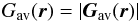 where
where 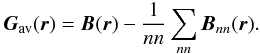 In the above definitions nn is the number of nearest neighbors for each site r and Bnn(r) is the magnetic field vector of these neighbors. Depending on the location of each site within the volume, the number of nearest neighbors nn can be nn = 3 − 6. The physical reason for selecting this criterion lies in the fact that large magnetic stresses favor magnetic reconnection in three dimensions, even in the absence of null points (Priest et al. 2003).
Mathematically, it can be shown that the selection of Gav as the critical quantity in our model relates to the diffusive term of the induction equation (see Isliker et al. 1998, for a detailed discussion). Let us write the induction equation in the form: 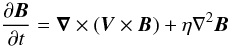 (2)where V is the plasma velocity and η the resistivity. The Laplacian of the magnetic field ∇2B(r) can be written as
  where r = (i,j,k). Letting m ≡ x,y,z we obtain
 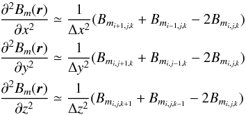 adopting a central finite-difference scheme and using the general case of a grid point having six nearest neighbors (nn = 6). Further assuming Δx = Δy = Δz = 1 (the grid-size) we have
 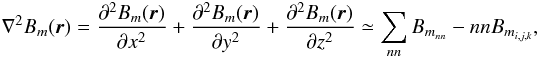 which yields ∇2B(r) as follows:
 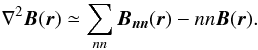 From the definition of the critical quantity Gav(r) it follows that
 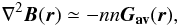 (3)therefore the critical quantity Gav(r) relates directly to the Laplacian ∇2B. The resistivity in the solar corona is almost zero everywhere except in regions where the discontinuities (and the local currents) reach a critical value. In these regions current-driven instabilities will enhance the resistivity by many orders of magnitude, and the second term in Eq. (2) will become dominant. The convective term ∇ × (V × B) of Eq. (2) will be further discussed in Sect. 3.4, where the driving module “LOAD” is described.
There are several ways to determine the threshold value for the critical quantity, above which a site is considered unstable:
-
1.
We apply a histogram method, by constructing the histogram ofthe Gav values in our grid. We then fit a Gaussian to this histogram and define the threshold Gcr as the field stress value, above which the histogram deviates from the Gaussian.
-
2.
We define the threshold value (Gcr) for the whole grid, as the maximum Gavmax value throughout our volume, decreased slightly:
Gcr = Gavmax(1 − s)
where s ≪ 1.
-
3.
We define the threshold value (Gcr(z)) per height z, as thev maximum Gavmax value for each specific height, slightly decreased:
Gcr(z) = Gavmax(z)(1 − s)
where s ≪ 1.
-
4.
We define the threshold value as a function of height z, e.g.:
Gcr(z) = Gavmax(1 − s)exp(−z)
where s ≪ 1.
Here we present the results produced by the first (histogram) method, which yielded Gcr = 10 G for our sample, and shortly refer to the other threshold alternatives in Sect. 4. Every site r = (i,j,k) for which the inequality Gavi,j,k ≥ Gcr is satisfied is considered unstable and undergoes magnetic field restructuring under the rules implemented in the “RELAX” module. Given the definition of the critical threshold, instabilities sometimes occur even from the first iteration, after constructing the NLFF fields. This, however, does not incur any qualitative impact on the evolution of the system toward SOC or on the statistical results of the simulation.
3.3. “RELAX”: a redistribution module for magnetic energy
In case the instability criterion Gavi,j,k ≥ Gcr is met for a specific site i,j,k, then the vicinity of the unstable location undergoes a field restructuring, which follows the rules of Lu & Hamilton (1991): 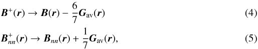 where the superscript + denotes the field components after the redistribution.
At this point it is important to investigate whether the redistribution rules as defined here violate basic physical laws, such as the zero-divergence requirement for the magnetic field. The initial magnetic configuration approximately satisfies the condition ∇·B = 0, as the field has been reconstructed using an NLFF field extrapolation. The question is whether the magnetic field after the redistribution imposed by rules (4), (5) still satisfies the same demand (∇·B + = 0). Taking the divergence of B + (r) and its neighbors  , we respectively find from relations (4) and (5)
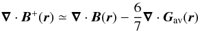
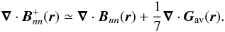 From the definition of Gav(r) we now have
 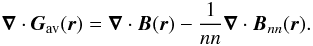 Substituting this into the above we find
 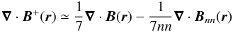 (6)
(6)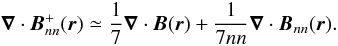 (7)Because ∇·B(r) ≃ ∇·Bnn(r) ≃ 0 from our first iteration (extrapolated fields), we find
  . Thus, the redistribution of the magnetic field maintains the divergence-free condition.
Isliker et al. (1998) show that the redistribution rules (4) and (5) implement local diffusion and after redistribution,  , so the instability at location r has been relaxed.
3.4. “LOAD”: the driver
After the system is completely relaxed, we introduce a driving mechanism that adds a magnetic field increment δB(r) at one randomly selected site r within our grid. The driving process complies with the following conditions:
-
 (8)This condition implies that the magnetic field increment is always perpendicular to the existing magnetic field B(r) at the randomly selected site r. Figure 1 provides a sketch of the suggested situation, depicting the directions of the plasma velocity V, the magnetic field B and the perpendicular magnetic field increment δB. We note that the condition described by Eq. (8) is compatible with two physical scenarios: (a) that Alfven waves may have been excited locally; or (b) that, according to the convective term ∇ × (V × B) of the induction Eq. (2), a magnetized plasma upflow occurs in the AR, out from the photosphere.
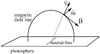
Fig. 1 Typical configuration of a magnetic loop anchored in the photosphere. The magnetic field vector B is perpendicular to an assumed plasma outflow velocity V. The model driver requires that the magnetic field increments δB are always perpendicular to the existing magnetic field B.
-
2.
 (9)This is a typical condition known to allow the system to reach the SOC state, without this state being influenced by the loading process (Bak et al. 1987). As also shown by Lu & Hamilton (1991), decreasing the driving rate by making the magnetic field increments even smaller, increases the average time between subsequent events. For the results presented here we have used a fixed ϵ = 0.3.
 -
3.
 (10)This condition should guarantee that the divergence of the magnetic field is approximately kept to zero during the loading process, as was done during the redistribution of the magnetic field (RELAX module). To implement the condition, a first-order, left finite-difference scheme is used. In this way, however, condition (10) does not provide an adequate guarantee for a divergence-free magnetic field in the selected site’s vicinity. This is a known problem, which can be tackled by working with the vector potential A, with ∇ × A = B, instead of the magnetic field B directly (see e.g. Lu et al. 1993; Galsgaard 1996; Isliker et al. 2000, 2001). Because our study uses observed vector magnetograms as initial conditions, we naturally work with the known magnetic fields, rather than the unknown vector potential. Thus, Eq. (10) only provides a low-order approximation towards a divergence-free magnetic field. To monitor how effective condition (10) is, we introduce a “Weighted Nabla Dot B” (WNDB) monitoring parameter, as follows:
  By definition, WNDB is a dimensionless quantity, lying in the range 0 ≤ WNDB ≤ 1. Monitoring WNDB during our simulation will provide evidence on whether condition (10) can be considered adequate for keeping the magnetic field within our volume approximately divergence-free. In the following, we tolerate a departure from zero of up to 20% (WNDB ≤ 0.2) for a still a roughly divergence-free magnetic field.
3.5. Model parameters
Linking the above-mentioned modules in one consistent simulation, we construct a relatively simple algorithm and monitor the flare duration, the peak energy, and the total energy, the distribution functions of which we intend to compare to those of observational data. If an instability is identified (DISCO) – either in the original magnetic configuration generated by the initial extrapolated magnetogram (EXTRA) or from an increment δB randomly added at a grid point (LOAD) – the possible chain of instabilities that follows is left to completely relax (RELAX) before an additional magnetic field increment is randomly placed (LOAD), possibly causing a new instability. This rule takes the observational fact into account that the lifetime of a flare is much shorter than the evolution timescale of an AR. Successive grid scans may be required for an instability to be completely relaxed. Each scanning corresponds to one timestep, therefore the relaxation of an event may be accomplished in more than one timesteps. Each loading event according to the equation set (8)−(10) triggers a new iteration. The duration of an event is defined as the total number of timesteps the event lasted, from its onset until its complete relaxation. The accumulated released energy during the event provides the total energy of an event, whereas the peak during an event yields the peak energy/luminosity of an event.
The simulation results presented in the next section have been performed using a 32 × 32 × 32 cubic grid with “open” boundaries in the relaxation events (see Isliker et al. 2001, for a detailed discussion on open boundary conditions). Each simulation is driven for 3 × 10⁵ iterations, which equals the times that LOAD module is being called during the simulation. This mechanism allows the production of multiple subsequent flares in each AR. In all cases the critical threshold Gcr was kept fixed and equal to 10 G.
4. Results
Applying our flare simulation model to our 11-event-database, we find that in all cases the simulated ARs reached the SOC state. An indication of whether and when the SOC state is reached is obtained by monitoring the quantity  , namely, the volume average of the critical quantity Gav. During the continuous driving of the system and the subsequently generated avalanches, increases gradually. When the system reaches the SOC state, stabilizes around a value that depends on the system’s characteristics. For the loading method used in our model (new magnetic field increments are only added when a previously triggered avalanche has decayed), the value around which stabilizes is slightly lower than the threshold value Gcr. A second indication that the system has reached the SOC state is that the total energy of the system tends toward an asymptotic value. This is because SOC is a statistically stationary state. Figure 2 shows the value over 3 × 10⁵ timesteps for AR10570. is constantly increasing up to timestep 1.4 × 10⁵, thereafter stabilizing at ~9.80 G ≲ Gcr = 10 G. Similarly, Fig. 3 shows the logarithm of the total magnetic energy throughout the volume Etotaft after each scan of the grid for possible redistributions. Following , Etotaft increases until a stable state is reached. The stabilization of both and Etotaft is a solid indication that SOC has been reached for AR10570. The same behavior is seen for all ARs included in our sample.
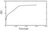 |
Fig. 2 Average Laplacian |
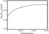 |
Fig. 3 Diagram of log 10(Etotaft) after each redistribution for AR10570. Like |
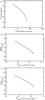 |
Fig. 4 Distribution functions for the event duration (Fig. 4a), the peak energy Epeak (Fig. 4b), and the total energy Etotal (Fig. 4c) for AR10050. The energies in b) and c) are calculated in physical units (ergs). |
SOC is generally characterized by intermittent transport events (avalanches), whose sizes range from very small (a single neighborhood) up to comparable to the system size. Power-law frequency distributions describe the parameters of these avalanches. It is thus reasonable to expect that since all 11 ARs in our sample have reached the SOC state under the imposed driving rules, they should all produce distribution functions for the flare duration, peak energy, and total energy, which either follow pure power laws or functions including a power-law part (e.g. power laws with exponential rollover). The functions tested against the model results for all flare parameters (flare duration, peak energy, total energy) were single power laws, double power laws, power laws with exponential rollover, and exponential functions. In order to define the best-fitting function per case, we made least square fits and performed chi-square goodness-of-fit tests.
Figures 4 and 5 are typical examples of our general results. Figure 4 depicts the distribution functions of duration (Fig. 4a), peak energy (Fig. 4b), and total energy (Fig. 4c)) for AR10050. The duration distribution follows a double power law with index − 1.80 ± 0.18 for the flatter part and − 4.03 ± 0.29 for the steeper part. Both the peak and total energy distribution functions follow single power laws with indices − 1.63 ± 0.15 and − 1.45 ± 0.13, respectively. Figure 5 depicts the distribution functions of duration (Fig. 5a), peak energy (Fig. 5b), and total energy (Fig. 5c) for AR9415. Here the duration distribution follows a power law with an exponential rollover. The power-law index is − 1.42 ± 0.18. The peak and total energy distribution functions follow again single power laws with indices − 1.84 ± 0.18 and − 1.50 ± 0.13, respectively.
Power-law indices and respective chi-square probabilities derived by the best-fit functions for the flare duration for the 11 ARs comprising our sample.
From the above, flare-duration distributions appear to be best-fitted either by power laws or by power laws with exponential rollovers. By comparing the chi-square values and respective probabilities for single power laws, double power laws, and power laws with exponential rollover, it is concluded that three of our ARs follow double power laws (AR9635, AR10050, AR10488), while the rest are best fitted by power laws with exponential rollovers. These indices are summarized in Table 1, along with the respective probabilities. The values shown in Table 1 refer to the fitting achieved against the entire distribution function in all cases (all bins included). Single power laws fail to describe the model duration distribution functions in all cases, whereas exponential functions only fit the tail of the generated model curves. In cases where a double power law is the best fit (AR9635, AR10050, AR10488), the mean index for the flat power law is − 1.90, whereas the mean index for the steep power law is − 4.32. When power laws with exponential rollover are best fitting (remaining ARs), then the mean value for the power law index is − 1.01. Standard deviations (σ2) to these mean values are given in the last row of this table.
Power-law indices and respective chi-square probabilities derived by fitting a single power law to the peak flare energy for the 11 ARs comprising our sample.
Although single power laws are not the optimum functions to fit the modeled flare duration, they are undoubtedly the best-fitting theoretical functions for the peak energy and the total flare energy. As shown in Table 2 for the peak flare energy and in Table 3 for the total flare energy, the average value for Epeak is −1.80, whereas the average index value for Etotal is −1.57. The standard deviation (σ2) of these mean values is given in the last row of these tables.
Power-law indices and respective chi-square probabilities derived by fitting a single power law to the total flare energy for the 11 ARs comprising our sample.
Figure 6 illustrates the magnetic energy released Erel for a specific period of 10 000 timesteps after SOC has been reached for AR10570. As the added driver increments δB assume low and random values, the waiting time from one flaring event to another varies. Figures 7 and 8 show a 3d representation of the emerging magnetic discontinuities during a large and a smaller avalanche, respectively, simulated for AR10247 after SOC has been reached. In the former case, the avalanche during its early stages generates 140 discontinuities (Fig. 7a), evolves further (Fig. 7b) with 281 discontinuities, peaks (Fig. 7c) with 425 discontinuities, and decays (Figs. 7d − f) with 184, 51, and 18 discontinuities, respectively. The total event duration is 341 steps. The total duration of the smaller event (Fig. 8) is 90 steps. The event during its early stages generates six discontinuities (Fig. 8a), peaks (Fig. 8b) with 15 discontinuities, and decays (Figs. 8c,d) with ten and six discontinuities, respectively.
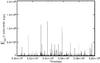 |
Fig. 6 Time series of the total magnetic energy released Erel (in 1.033 × 1025 ergs) from the simulated AR10570 after the SOC state has been reached. The time series shown consists of 10 000 timesteps for better detail. |
Finally, it is interesting to investigate whether our model consistently reproduces the distribution functions of the flaring events actually observed in the ARs in our sample. For our comparison we used the solar X-ray flare catalog from the GOES satellite (http://www.ngdc.noaa.gov/stp/SOLAR/ftpsolarflares.html, item 3). The flaring events recorded in this database lie in the class range B − X and are summarized in Table 4 for each AR. However, to construct the distribution functions of flare parameters we need enough statistics, reflected in large flare numbers. Regardless of its flare productivity, a single AR is unlikely to provide these numbers. For this reason and for the sake of comparison, we have merged all observed flares in all studied ARs into a single flare sequence with a total of 154 events (sum of all flares in Table 4). Table 5 shows the statistical results of our analysis for flare durations. As flare duration, we define the observed onset-to-end elapsed time. The best-fitting function is not easily discernible in this case, as all candidate functions (single power law, double power law, and power law with exponential rollover) fit the observational data fairly well. Figure 9 depicts the fit between the observed flare durations against a double power law (Fig. 9a) and a power law with exponential rollover (Fig. 9b). In the former case (Fig. 9a) the calculated index is −1.67 ± 0.09 for the smooth part and −3.37 ± 0.25 for the steep part, whereas in the latter case (Fig. 9b) the power-law index yields −1.28 ± 0.11. It is apparent that the dynamical range of the power law in Fig. 9a is very limited, but it is shown here for comparison purposes. To achieve this comparison, we merge the model results of the separate runs per AR into one common database. Figure 10 depicts the fit between the merged model flare durations for all ARs in our sample against a double power law (Fig. 10a) and a power law with exponential rollover (Fig. 10b). In the former case the calculated index is −1.78 ± 0.27 for the smooth part and −3.91 ± 0.42 for the steep part, whereas in the latter case the power-law index yields −1.13 ± 0.12. By comparing the results depicted in Fig. 9 (observational data) and Fig. 10 (merged model data), we conclude that the power law indices for the observational data are close to our model’s values for the double power law and power law with exponential rollover fits. This is not the case for the single power-law fitting, which yields an index of −1.70 for the GOES data. The best agreement between the observed and the simulated flares is, therefore, achieved when the attempted fit is not a single power law, but either a double power law or a power law with an exponential rollover. Table 6 is similar to Table 5, summarizing the indices resulting from the merged model data.
Although our findings show good alignment with both previous models and observations, it is crucial to crosscheck the physical soundness of our algorithm. As mentioned in Sect. 3.4, loading rule (10) does not by itself guarantee that the magnetic field remains divergence-free during the entire simulation. WNDB is therefore determined in order to monitor the magnetic field divergence throughout the loading and redistribution process. Figure 11 presents the evolution of WNDB during the 3 × 10⁵ timesteps of our simulation for AR10247. In the beginning, WNDB is close to zero, as our initial condition is the extrapolated NLFF (and therefore approximately divergence-free) magnetic field. As time elapses, ∇·B starts deviating from zero, but WNDB remains under 0.20 during the entire simulation. This holds for all ARs in our sample. Therefore, our model retains the magnetic field approximately divergence-free throughout the simulation.
Furthermore, it is worth investigating whether the use of alternative threshold definitions incurs any qualitative changes in the presented results. As an example, we apply the second threshold definition of Sect. 3.2 to AR10247. In this case, Gcr = Gavmax(1 − s) ≃ 30 G. Figure 12 shows that even with this threshold definition, increases gradually until timestep 1.3 × 10⁵, after which the SOC state is reached, and stabilizes around approximately 29.95, which is lower than the critical threshold Gcr = 30. The statistical properties of the generated distribution functions remain unchanged. This is also valid when switching from a 32 × 32 × 32 grid towards larger volumes (e.g. a 64 × 64 × 64 grid).
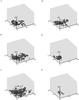 |
Fig. 7 3d representation of the emerging magnetic discontinuities during an avalanche in AR10247. The total duration of this event is 341 steps. During the early stages, the avalanche generates numerous discontinuities (140 in a)), evolves with 281 discontinuities b), peaks with 425 discontinuities c), and decays with 184 discontinuities d), 51 discontinuities e), and 18 discontinuities f). |
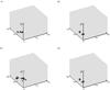 |
Fig. 8 3d representation of the emerging magnetic discontinuities during an avalanche in AR10247. The total duration of this event is 90 steps. During the early stages, the event generates a small number or discontinuities (6 in a)), peaks with 15 discontinuities b), and decays with 10 discontinuities c) and 6 discontinuities d). |
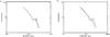 |
Fig. 9 Observed distributions of GOES flare durations for all ARs in our sample. Fit is attempted using a double power law a) and a power law with an exponential rollover b). The double power law fit yields an index equal to −1.67 ± 0.09 for the flat part and −3.37 ± 0.25 for the steep part, whereas the fit with the power law and the exponential rollover yields a scaling index −1.28 ± 0.11. |
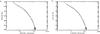 |
Fig. 10 Distributions of simulated flare durations for all ARs in our sample. Fit is attempted using a double power law a) and a power law with an exponential rollover b). The double power law fit yields an index equal to −1.78 ± 0.27 for the flat part and −3.91 ± 0.42 for the steep part, whereas the fit with the power law and the exponential rollover yields a scaling index −1.13 ± 0.12. |
GOES X-ray data for the number and class of observed flares in the ARs used in our simulations.
5. Discussion and conclusions
This study simulates the flaring activity of 11 solar ARs in terms of a refined CA model. The modules comprising this integrated flare model are summarized below
-
1.
We extrapolated the magnetic field from the photosphericboundary of 11 IVM magnetograms resampledon a 32 × 32 grid, through a nonlinear force-free optimization algorithm with preprocessing at the photospheric level (module “EXTRA”, refer to Sect. 3.1 for details).
-
2.
We identified the unstable locations that will dissipate magnetic energy in our grid when the approximated magnetic field Laplacian Gav(r) at site r exceeds a specific threshold Gcr (module “DISCO”, refer to Sect. 3.2 for details).
-
3.
In case magnetic discontinuities are identified (either directly after the initialization or after each loading), the magnetic energy was redistributed such that the instabilities are completely relaxed (module “RELAX” refer to Sect. 3.3 for details).
-
4.
Further loading within our system was allowed, when a previously triggered avalanche has completely decayed. In this case, LOAD added a random magnetic field increment δB(r) at a random site r within our grid according to the rules described in Sect. 3.4.
The algorithm was allowed to run for 3 × 10⁵ timesteps, which is sufficient for all simulated ARs to both reach the SOC state and provide sufficient event statistics after the SOC state had been reached. The enhancements of our flare simulation model in comparison to previous SOC models of solar flares follow
-
The initial boundary conditions are not arbitrary, but stem fromreal solar magnetograms.An NLFF field extrapolation isused to reconstruct the initial magnetic configuration generatedfrom the observed 11 ARs, retaining physicalrequirements to the best possible extent, such as the minimizationof the Lorentz force and the magnetic field divergence.
Table 5Power-law indices and respective chi-square probabilities derived by fitting several functions to the flare durations derived from the merged GOES observational data for the 11 ARs comprising our sample.
Table 6Power-law indices and respective chi-square probabilities derived by fitting several functions to the flare durations derived from the merged model data for the 11 ARs comprising our sample.
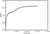
Fig. 11 Evolution of WNDB during the 300 000 timesteps of our simulation for AR10247.
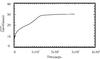
Fig. 12 Diagram of the average
value over the grid for 3 × 10⁵ timesteps for AR10247 when the threshold definition is Gcr = Gavmax(1 − s) ≃ 30 G. -
Given that the simulation commences from observed magnetograms, it is now possible for our CA model to remove the restriction of arbitrary energy units (see e.g. the remarks within Georgoulis et al. 2001). This gives us the opportunity to directly compare the model with the observed energy content per flare, thus leaving time as the only arbitrary quantity in our simulation.
-
Our model follows the principles of Lu & Hamilton (1991) to a significant degree. The rules obeyed during both the magnetic energy redistribution and the further driving of the system are designed in such a way that the magnetic field divergence is within tolerated limits. This has not been the case in the early CA models (Vlahos 1995; Georgoulis & Vlahos 1996, 1998) and has only been touched in advanced CA approaches through the use of the vector potential A instead of the magnetic field B in combination with an improved way of calculating the derivatives (Isliker et al. 2000, 2001).
-
The driving mechanism attempts to mimic not only photospheric convection as proposed by Parker (1988, 1989, 1993), but also coronal evolution, such as turbulence and current sheet interaction. In this sense, locations throughout the simulation box are randomly chosen to be perturbed. Via either localized Alfven waves or larger-scale turbulent flows (Einaudi et al. 1996; Rappazzo et al. 2008), turbulence leads to current-sheet interaction that may trigger an avalanche observed as a flare, depending on the local magnetic conditions. Naturally, though, due to the larger accumulation of magnetic free energy close to the photosphere (Regnier & Priest 2007) photospheric convection and systematic photospheric motions (e.g. shear) should be the drivers of most coronal instabilities. Our driving mechanism should be further revised to account for systematic photospheric flows. This future step is important because (1) it has been argued that the distribution and energy content of magnetic discontinuities in a given photospheric boundary can explain the statistical properties of flares (Vlahos & Georgoulis 2004) and (2) investigating possible correlations between the photospheric driver and the corresponding coronal active region reveals the strong nonlinearity of active-region magnetic configurations that hinders correlations between photospheric and coronal structures (Dimitropoulou et al. 2009). The latter patterns, however, have a crucial impact on the expected dynamical activity of the system, namely, the magnetic energy release and the subsequent particle acceleration processes (Vlahos et al. 2004).
-
The derived results can be directly compared with flare observations, because the simulation uses extrapolated fields from observed vector magnetograms as initial conditions. At this point, we once again stress that the X-ray flares recorded by GOES for each AR do not comprise a statistically reliable sample. Therefore, in order to make such a comparison possible, we merged the GOES flare data of all 11 ARs in our sample into one database, comprising 154 flares.
Our results show that under the imposed driving and redistribution rules, all examined ARs reach the SOC state. The retrieved distribution functions for event duration are best described by either double power laws or power laws with exponential rollover, although single power laws are also applicable for the merged data. The peak energy and total energy clearly follow single power laws. The power-law indices for durations and energies as presented in Tables 1 − 3 lie in the well-known ranges documented consistently in numerous past studies, including Georgoulis et al. (2001). In this study, Georgoulis et al. compare their SOC model with data from the Danish Wide Angle Telescope for Cosmic Hard X-rays (WATCH) collected during the maximum of the solar cycle 21. Figure 1 in the cited work shows that the peak and total energy of the observed flares follow single power-law distribution functions with indices −1.59 and −1.39 respectively, whereas the flare duration distribution function is considered to either follow a double power law (with index −1.15 for the flat and −2.25 for the steep part) or a power law with exponential rollover (with power law index −1.09). These results agree with our findings. Although our model generates flare duration distribution functions with indices in alignment with the ones presented in Georgoulis & Vlahos (1998), we did not attempt here to reproduce two key findings of Georgoulis & Vlahos (1998), namely the variability of the scaling indices as a result of the driver’s variability and the two distinct event populations. In the cited study, the peak and total energy distribution functions follow double power laws. The steeper part of them corresponds to the signature of a “soft” flare population (nanoflares), whereas the flatter part is attributed to microflares and flares.
Although this work overcomes major drawbacks of many previous CA models, such as retaining the value of the magnetic field divergence close to zero throughout the simulation, there are still some points that can lead to discrepancies. First and foremost, the determination of the threshold value Gcr can slightly influence the exponents of the retrieved power laws, although it cannot cause any qualitative change to their appearance; that is the known flare statistical properties will always follow power-law distributions, independent of the threshold value imposed. The histogram method presented in Sect. 3.2 eliminates the arbitrary selection of Gcr to an extent. We also investigated whether the rebinning of our grid to the size of 32 × 32 × 32 influences our results in comparison with larger grids (e.g. 64 × 64 × 64), and we found that the differences in the power-law indices lie within the inferred uncertainties. Finally, for the comparison with the observational data, we have already stressed that this is a preliminary attempt given that the number of GOES X-ray flares across all investigated ARs does not produce enough statistics.
The discussion regarding the validity of the CA models when it comes to the simulation of physical processes in complex systems a long-running. As discussed by Isliker et al. (1998), the essence of CA modeling is to describe complex systems, which comprise a large number of interacting subsystems, assuming that the global dynamics described statistically are not sensitive to the fine structure of the elementary processes. Stricter approaches such as MHD, on the other hand, are based on a precise description of the elementary processes through detailed differential equations. Both approaches have been shown to exhibit drawbacks and advantages. The CA approach does not provide any insight into the local processes or over short time intervals, but it reproduces the global statistics. MHD reveals details about the local processes, but coupling them to a global description is a formidable task. In this sense, the two approaches are complementary, and there have been indeed various attempts to either combine them (e.g. Longope & Noonan 2000), or interpret CA models as discretized MHD equations (Isliker et al. 1998; Vassiliadis et al. 1998). Even more extended CA models, like the X-CA model described by Isliker et al. (2001), have achieved consistency with MHD to a greater extent. Our CA model will opt to incorporate and utilize meaningful modeling developments into a more concrete, “integrated” flare model.
Acknowledgments
We are grateful to Thomas Wiegelmann who kindly contributed his NLFF extrapolation code to this analysis. Xenophon Moussas and Dafni Strintzi are acknowledged for their constructive comments in the course of this work. Additionally, IVM Survey data are made possible through the staff of the U. of Hawaii, supported by the Air Force Office of Scientific Research, contract F49620-03-C-0019. IVM Survey data are based upon work supported by the National Science Foundation under Grant No. 0454610. Any opinions, findings, and conclusions or recommendations expressed in this material are those of the author(s) and do not necessarily reflect the views of the National Science Foundation (NSF). Finally, we thank the anonymous referee whose help significantly improved the paper.
References
- Bak, P., Tang, C., & Wiesenfeld, K. 1987, Phys. Rev. Lett., 59, 381 [NASA ADS] [CrossRef] [PubMed] [Google Scholar]
- Biesecker, D. A. 1994, Ph.D. Thesis, University of New Hampshire [Google Scholar]
- Bromund, K. R., McTiernan, J. M., & Kane, S. R. 1995, ApJ, 455, 733 [NASA ADS] [CrossRef] [Google Scholar]
- Crosby, N. B., Aschwanden, M. J., & Dennis, B. R. 1993, Sol. Phys., 143, 275 [NASA ADS] [CrossRef] [Google Scholar]
- Datlowe, D. W., Elcan, M. J., & Hudson, H. S. 1974, Sol. Phys., 39, 155 [NASA ADS] [CrossRef] [Google Scholar]
- Dennis, B. R. 1985, Sol. Phys., 100, 465 [NASA ADS] [CrossRef] [Google Scholar]
- DeRosa, M. L., Schrijver, C. J., Barnes, G., et al. 2009, ApJ, 696, 1780 [Google Scholar]
- Dimitropoulou, M., Georgoulis, M., Isliker, H., et al. 2009, A&A, 505, 1245 [NASA ADS] [CrossRef] [EDP Sciences] [Google Scholar]
- Einaudi, G., Velli, M., Politano, H., & Pouquet, A. 1996, ApJ, 457, L113 [NASA ADS] [CrossRef] [Google Scholar]
- Galsgaard, K. 1996, A&A, 315, 312 [NASA ADS] [Google Scholar]
- Georgoulis, M. K. 2005, ApJ, 629, 69 [Google Scholar]
- Georgoulis, M. K., & Vlahos, L. 1996, ApJ, 469, L135 [NASA ADS] [CrossRef] [Google Scholar]
- Georgoulis, M. K., & Vlahos, L. 1998, ApJ, 336, 721 [Google Scholar]
- Georgoulis, M. K., Kluiving, R., & Vlahos, L. 1995, Phys. A, 218, 191 [CrossRef] [Google Scholar]
- Georgoulis, M. K., Vilmer, N., & Corsby, N. B. 2001, A&A, 367, 326 [NASA ADS] [CrossRef] [EDP Sciences] [Google Scholar]
- Harvey, K. L., & Zwaan, C. 1993, Sol. Phys., 148, 85 [NASA ADS] [CrossRef] [Google Scholar]
- Isliker, H., Anastasiadis, A., Vassiliadis, D., & Vlahos, L. 1998, A&A, 335, 1085 [NASA ADS] [Google Scholar]
- Isliker, H., Anastasiadis, A., & Vlahos, L. 2000, A&A, 363, 1134 [NASA ADS] [Google Scholar]
- Isliker, H., Anastasiadis, A., & Vlahos, L. 2001, A&A, 377, 1068 [NASA ADS] [CrossRef] [EDP Sciences] [Google Scholar]
- Isliker, H., Anastasiadis, A., & Vlahos, L. 2002, ESA SP-506, 6411 [Google Scholar]
- Lin, R. P., Schwartz, R. A., Kane, S. R., Pelling, R. M., & Hurly, K. C. 1984, ApJ, 283, 421 [NASA ADS] [CrossRef] [Google Scholar]
- Longope, D. W., & Noonan, E. J. 2000, ApJ, 542, 1088 [NASA ADS] [CrossRef] [Google Scholar]
- Lu, E. T., & Hamilton, R. J. 1991, ApJ, 380, L89 [NASA ADS] [CrossRef] [Google Scholar]
- Lu, E. T., Hamilton, R. J., McTiernan, J. M., & Bromund, K. R. 1993, ApJ, 412, 841 [NASA ADS] [CrossRef] [Google Scholar]
- MacKinnon, A. L., & Macpherson, K. P. 1997, A&A, 326, 1228 [NASA ADS] [Google Scholar]
- Mickey, D. L., Canfield, R. C., LaBonte, B. J., et al. 1996, Sol. Phys., 168, 229 [Google Scholar]
- Parker, E. N. 1988, ApJ, 330, 474 [Google Scholar]
- Parker, E. N. 1989, Sol. Phys., 121, 271 [NASA ADS] [CrossRef] [Google Scholar]
- Parker, E. N. 1993, ApJ, 414, 389 [NASA ADS] [CrossRef] [Google Scholar]
- Polygiannakis, J. M., Nikolopoulou, A., Preka-Papadima, P., Moussas, X., & Hilaris, A. 2002, ESA SP-505, 541 [Google Scholar]
- Priest, E. R., Hornig, G., & Pontin, D. I. 2003, J. Geophys. Res. Space Phys., 108(A7), 1285 [NASA ADS] [CrossRef] [Google Scholar]
- Rappazzo, A. F., Velli, M., Einaudi, G., & Dahlburg, R. B. 2008, ApJ, 677, 1348 [NASA ADS] [CrossRef] [Google Scholar]
- Regnier, S., & Priest, E. R. 2007, A&A, 468, 701 [NASA ADS] [CrossRef] [EDP Sciences] [Google Scholar]
- Shimizu, T. 1995, PASJ, 47, 251 [NASA ADS] [Google Scholar]
- Sturrock, S., Kaufmann, P., Moore, P. L., & Smith, D. F. 1984, Sol. Phys., 94, 341 [NASA ADS] [CrossRef] [Google Scholar]
- Vassiliadis, D., Vlahos, L., & Georgoulis, M. 1998, ApJ, 509, L53 [NASA ADS] [CrossRef] [Google Scholar]
- Vilmer, N. 1987, Sol. Phys., 111, 207 [NASA ADS] [CrossRef] [Google Scholar]
- Vlahos, L., & Georgoulis, M. K. 2004, ApJ, 603, 61 [Google Scholar]
- Vlahos, L., Georgoulis, M. K., Kluiving, R., & Paschos, P. 1995, A&A, 299, 897 [NASA ADS] [Google Scholar]
- Vlahos, L., Fragos, T., Isliker, H., & Georgoulis, M. K. 2002, ApJ, 575, 87 [Google Scholar]
- Vlahos, L., Isliker, H., & Lepreti, F. K. 2004, ApJ, 608, 540 [NASA ADS] [CrossRef] [Google Scholar]
- Wheatland, M. S., Staurrock, P. A., & Roumeliotis, G. 2000, ApJ, 540, 1150 [Google Scholar]
- Wiegelmann, T. 2004, Sol. Phys., 219, 87 [NASA ADS] [CrossRef] [Google Scholar]
- Wiegelmann, T. 2008, J. Geophys. Res., 113, A03S02 [Google Scholar]
- Wiegelmann, T., Inhester, B., & Sakurai, T. 2006, Sol. Phys., 233, 215 [NASA ADS] [CrossRef] [Google Scholar]
All Tables
Power-law indices and respective chi-square probabilities derived by the best-fit functions for the flare duration for the 11 ARs comprising our sample.
Power-law indices and respective chi-square probabilities derived by fitting a single power law to the peak flare energy for the 11 ARs comprising our sample.
Power-law indices and respective chi-square probabilities derived by fitting a single power law to the total flare energy for the 11 ARs comprising our sample.
GOES X-ray data for the number and class of observed flares in the ARs used in our simulations.
Power-law indices and respective chi-square probabilities derived by fitting several functions to the flare durations derived from the merged GOES observational data for the 11 ARs comprising our sample.
Power-law indices and respective chi-square probabilities derived by fitting several functions to the flare durations derived from the merged model data for the 11 ARs comprising our sample.
All Figures
|
Fig. 1 Typical configuration of a magnetic loop anchored in the photosphere. The magnetic field vector B is perpendicular to an assumed plasma outflow velocity V. The model driver requires that the magnetic field increments δB are always perpendicular to the existing magnetic field B. |
| In the text | |
|
Fig. 2 Average Laplacian |
| In the text | |
|
Fig. 3 Diagram of log 10(Etotaft) after each redistribution for AR10570. Like |
| In the text | |
|
Fig. 4 Distribution functions for the event duration (Fig. 4a), the peak energy Epeak (Fig. 4b), and the total energy Etotal (Fig. 4c) for AR10050. The energies in b) and c) are calculated in physical units (ergs). |
| In the text | |
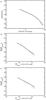 |
Fig. 5 Same as Fig. 4 for AR9415. |
| In the text | |
|
Fig. 6 Time series of the total magnetic energy released Erel (in 1.033 × 1025 ergs) from the simulated AR10570 after the SOC state has been reached. The time series shown consists of 10 000 timesteps for better detail. |
| In the text | |
|
Fig. 7 3d representation of the emerging magnetic discontinuities during an avalanche in AR10247. The total duration of this event is 341 steps. During the early stages, the avalanche generates numerous discontinuities (140 in a)), evolves with 281 discontinuities b), peaks with 425 discontinuities c), and decays with 184 discontinuities d), 51 discontinuities e), and 18 discontinuities f). |
| In the text | |
|
Fig. 8 3d representation of the emerging magnetic discontinuities during an avalanche in AR10247. The total duration of this event is 90 steps. During the early stages, the event generates a small number or discontinuities (6 in a)), peaks with 15 discontinuities b), and decays with 10 discontinuities c) and 6 discontinuities d). |
| In the text | |
|
Fig. 9 Observed distributions of GOES flare durations for all ARs in our sample. Fit is attempted using a double power law a) and a power law with an exponential rollover b). The double power law fit yields an index equal to −1.67 ± 0.09 for the flat part and −3.37 ± 0.25 for the steep part, whereas the fit with the power law and the exponential rollover yields a scaling index −1.28 ± 0.11. |
| In the text | |
|
Fig. 10 Distributions of simulated flare durations for all ARs in our sample. Fit is attempted using a double power law a) and a power law with an exponential rollover b). The double power law fit yields an index equal to −1.78 ± 0.27 for the flat part and −3.91 ± 0.42 for the steep part, whereas the fit with the power law and the exponential rollover yields a scaling index −1.13 ± 0.12. |
| In the text | |
|
Fig. 11 Evolution of WNDB during the 300 000 timesteps of our simulation for AR10247. |
| In the text | |
|
Fig. 12 Diagram of the average |
| In the text | |
Current usage metrics show cumulative count of Article Views (full-text article views including HTML views, PDF and ePub downloads, according to the available data) and Abstracts Views on Vision4Press platform.
Data correspond to usage on the plateform after 2015. The current usage metrics is available 48-96 hours after online publication and is updated daily on week days.
Initial download of the metrics may take a while.