| Issue |
A&A
Volume 529, May 2011
|
|
|---|---|---|
| Article Number | A71 | |
| Number of page(s) | 11 | |
| Section | Planets and planetary systems | |
| DOI | https://doi.org/10.1051/0004-6361/201014194 | |
| Published online | 05 April 2011 | |
New 3D thermal evolution model for icy bodies application to trans-Neptunian objects
1
LESIA, Observatoire de Paris – Section Meudon, 2 Place J. Janssen, 92195 Meudon Principal Cedex, France
2
UCLA, Department of Earth and Space Sciences, 595 Charles E. Young Drive East, Los Angeles CA 90095, USA
e-mail: This email address is being protected from spambots. You need JavaScript enabled to view it.
3 Los Alamos National Laboratory, Space Sciences and Applications, ISR-1, Mail Stop D-466, USA
4
Lunar and Planetary Institute, 3600 Bay Area Boulevard, Houston TX 77058, USA
5
Università di Perugia, Dipartimento di Scienze della Terra, 06123 Perugia, Italy
6
INAF-IFSI, via del Fosso del Cavaliere, 00133 Roma, Italy
7
INAF-IASF, via del Fosso del Cavaliere, 00133 Roma, Italy
8
Jet Propulsion Laboratory, 4800 Oak Grove Drive, MS 183-301, Pasadena, CA 91109, USA
Received: 3 February 2010
Accepted: 4 February 2011
Abstract
Context. Thermal evolution models have been developed over the years to investigate the evolution of thermal properties based on the transfer of heat fluxes or transport of gas through a porous matrix, among others. Applications of such models to trans-Neptunian objects (TNOs) and Centaurs has shown that these bodies could be strongly differentiated from the point of view of chemistry (i.e. loss of most volatile ices), as well as from physics (e.g. melting of water ice), resulting in stratified internal structures with differentiated cores and potential pristine material close to the surface. In this context, some observational results, such as the detection of crystalline water ice or volatiles, remain puzzling.
Aims. In this paper, we would like to present a new fully three-dimensional thermal evolution model. With this model, we aim to improve determination of the temperature distribution inside icy bodies such as TNOs by accounting for lateral heat fluxes, which have been proven to be important for accurate simulations. We also would like to be able to account for heterogeneous boundary conditions at the surface through various albedo properties, for example, that might induce different local temperature distributions.
Methods. In a departure from published modeling approaches, the heat diffusion problem and its boundary conditions are represented in terms of real spherical harmonics, increasing the numerical efficiency by roughly an order of magnitude. We then compare this new model and another 3D model recently published to illustrate the advantages and limits of the new model. We try to put some constraints on the presence of crystalline water ice at the surface of TNOs.
Results. The results obtained with this new model are in excellent agreement with results obtained by different groups with various models. Small TNOs could remain primitive unless they are formed quickly (less than 2 Myr) or are debris from the disruption of larger bodies. We find that, for large objects with a thermal evolution dominated by the decay of long-lived isotopes (objects with a formation period greater than 2 to 3 Myr), the presence of crystalline water ice would require both a large radius (>300 km) and high density (>1500 kg m-3). In particular, objects with intermediate radii and densities would be an interesting transitory population deserving a detailed study of individual fates.
Key words: Kuiper belt: general / diffusion / methods: numerical
© ESO, 2011
1. Introduction
Trans-Neptunian objects (TNOs) and Centaurs are generally assumed to be pristine remnants of planets formation, thus holding clues to the early stages of the solar system evolution. However, it is still debated whether this assumption is correct and to what extent TNOs remain primitive. Observations are constantly carried out to investigate their surface properties (mainly composition and color) and physical parameters (such as size, mass, or rotation period), which is a difficult task owing to their great heliocentric distances and their resulting faintness (Barucci et al. 2008a).
The TNOs’ albedos and sizes can be constrained by thermal observations (Stansberry et al. 2008, and references therein). Masses and densities can be obtained by observing multiple systems (Noll et al. 2008, for a review). Some rotation periods and shapes have been determined through photometric lightcurves (Sheppard et al. 2008). When it comes to surface properties, broadband photometry has revealed a wide range of colors displayed by both TNO and Centaur populations (Doressoundiram et al. 2008; Tegler et al. 2008). Near-infrared spectroscopy has highlighted the variety of their surface compositions (Barucci et al. 2008b, for a review), as well as the presence of volatile ices (Cook et al. 2007; Barucci et al. 2008c).
These properties are commonly interpreted as the result of the competition between internal and external processes that alter the surfaces. Irradiation, for instance, causes the formation of a crust that shields the material underneath (Strazzulla et al. 1991; Brunetto & Roush 2008). Impact collisions can thus expose less irradiated material. Internal processes, such as comet-like activity or cryovolcanism, can act the same way by redepositing fresh, non-irradiated material on the surface (Belton & Melosh 2009). Some Centaurs effectively display cometary activity (Jewitt 2009), while it has only been suspected once (and never confirmed) on a TNO (Hainaut et al. 2000). Studying the thermal evolution of such objects could constrain the possibility of internal events (for example cometary activity) in the recent past, of which the effects on the surface compositions and colors could still be observable today.
Thermal simulations of icy bodies have been developed over the years to investigate the evolution of thermal properties based on the transfer of heat flux, the sublimation of ices, and the transport of gas through a porous matrix. Initially, 1D models of the heat diffusion equation and gas transport were developed with specific applications to comet nuclei, especially in the wake of the Giotto exploration of comet 1P/Halley (e.g. Fanale & Savail 1984; Herman & Podolak 1985; Espinasse et al. 1991; see Huebner et al. 2006, for a review). Over the last decade, more complexities were introduced, with a particular emphasis on accounting for the lateral conduction of heat toward a 3D resolution of the equations for spherical bodies (Enzian et al. 1997; Orosei et al. 1999; Cohen et al. 2003; Rosenberg & Prialnik 2007) and the nonspherical shapes of comet nuclei (Lasue et al. 2008).
The application of thermal evolution models to TNOs and Centaurs has shown that, after their formation and early evolution, the resulting bodies could almost be completely depleted of most volatile ices (DeSanctis et al. 2001; Merk & Prialnik 2006; McKinnon et al. 2008). Water ice could have completely crystallized or even melted, leading to a layered structure with a core depleted in pristine material and less processed outer layers. Since thermal evolution depends strongly on the object’s size, composition, and the abundance of radioactive isotopes, some amorphous ice could be preserved, and entire or partly primitive bodies can remain (differentiated cores and primitive outer layers).
Lateral heat fluxes are crucial to determining of the temperature distribution at the surface and inside icy bodies (Enzian et al. 1997). Orosei et al. (1999) compared results obtained with a 1D with those from a 2D model, and show that latitudinal heat conduction diverts energy from the equator to the poles, resulting in a lower equatorial temperature when the object is at perihelion. Some differences also appear in the longterm evolution of the surface average annual temperature, which increases at all latitudes from orbit to orbit. This pattern is completely absent from the results of the 1D model. Therefore, nonradial heat conduction can be the origin of a significant difference in the long-term evolution of a body, especially when it comes to temperature-dependent processes, such as the crystallization of amorphous ice or the sublimation/condensation of volatiles within the porous matrix. The chemical differentiation induced by solar illumination seems to be overestimated in 1D models.
An effort has thus been made to develop fully 3D models which are expected to give better constraints on the thermal evolution of icy bodies through more realistic treatment of insolation at the surface, and its effect on subsurface layers. These models can also account for a more realistic and complex treatment of the boundary conditions, such as heterogeneous albedo distribution at the surface. However, a realistic 3D model needs to solve the various equations simultaneously for all the elements of the 3D grid, which dramatically increases the computational time. Simplifications of the physical processes involved, therefore, must be made. For example, the gas production and flow in the interior of the bodies is not accounted for by Rosenberg & Prialnik (2007).
We developed an innovative 3D thermal evolution model using a mathematical formulation in spherical harmonics that reduces the computation time. By doing this, we expect to be able to increase the spatial resolution of the grid to improve the temperature determination, in particular for objects close to the Sun. The basic equations and the algorithm are described in Sect. 2, and physical parameters relevant to the modeling of TNOs and Centaurs are outlined in Sect. 3. Section 4 discusses the approximations and the validation of the model. Section 5 discusses the question of the presence/absence of amorphous and/or crystalline water ice at the surface of these objects.
2. Basic equations
2.1. Heat diffusion equation
We aim to evaluate the temperature distribution inside icy bodies such as TNOs and Centaurs, taking various thermal and physical processes into account such as the decay of radioactive isotopes and the exothermic crystallization of amorphous ice. We assume that the bodies are spheres made of porous water ice (amorphous and/or crystalline) and dust (silicates), homogeneously distributed within the ice matrix. Heat diffusion is computed for the three dimensions of the sphere: radial, latitudinal, and azimuthal. Sublimation/condensation of volatiles and gas flow in the porous matrix are not accounted for in the current version of the model. The heat conduction equation to be solved is, therefore, 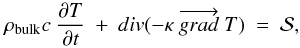 (1)where T [K] is the temperature distribution to be determined, ρbulk [kg m-3] the object’s bulk density, c [J kg-1 K-1] the material heat capacity, κ [W m-1 K-1] its effective thermal conductivity and
  the total heat source (see Sect. 2.3).
The heat diffusion equation can be expanded in spherical coordinates: 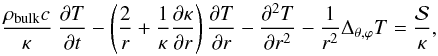 (2)with Δθ,ϕ the angular Laplacian operator, by neglecting the angular derivative of κ, ρbulk and c (see Sect. 3.3). We introduce spherical harmonics that allow a simple and natural expression of the temperature over a regular spherical grid. This has been used for the Earth and the Moon (Wierczorek 2007). Real spherical harmonics
  with θ ∈ [0,π ] the colatitude and ϕ ∈ [0,2π ] the longitude form an orthonormal basis of the Hilbert space of real-valued square integrable functions. Each spherical harmonic of degree l (l ∈ N) and order m (m ∈ Z,|m| ≤ l) is an eigenfunction of the angular Laplacian operator, associated with the eigenvalue − l(l + 1). They are defined as follows:
  (3)with αlm the orthonormalization coefficient,
  the Legendre polynomials and Φm(ϕ) the azimuthal function.
As a result, the expansion of the temperature on the basis of the real spherical harmonics gives 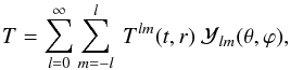 (4)which is exact as long as the degree l goes to infinity. Nonetheless, this ideal case cannot be reached for numerical reasons. We thus introduce a maximum degree lmax to cut the sum. The influence of this choice is discussed in Sect. 4.1. We then introduce the expansion in the heat diffusion equation:
  (5)with
  described in Sect. 2.3. We therefore obtain (lmax + 1)2 equations of Tlm(t,r), instead of one single 3D equation of T. These 1D equations are solved using a Crank-Nicholson numerical scheme, which is a stable, implicit technique.
2.2. Grid and boundary conditions
The body is virtually divided into elementary volumes by assuming a 3D-grid defined in the (r, θ, ϕ) spherical frame of reference, with θ ∈ [0,π] the colatitude and ϕ ∈ [0,2π] the longitude. The radial grid is chosen so as to minimize the discretization errors, with several samples near the surface, where the thermal gradients are strong: a thickness of a few centimeters is assumed for the first 100 layers (for example 0.5 cm for the first layer, then a linear increase in each layer thickness). This technique has already been used to model comet nuclei. The layers close to the surface suffer the largest variations in temperature on a small spatial scale from the solar illumination, with a skin depth of a few tens of centimeters (Huebner et al. 2006). In this case, the subsurface layers have usually a thickness of the order of a centimeter.
The sampling of the lateral 2D-(θ, ϕ) grid is constrained by using spherical harmonics, in particular the sampling theorem (Driscoll & Healy 1994) for the surface boundary condition (see Eq. (9)). Several thermal processes are considered to evaluate the thermal balance:
-
▸
solar illumination described by
 , with
  the Bond albedo, C⊙ the solar constant, dH the object’s heliocentric distance, and ξ the local zenith angle.
 -
▸
thermal emission εσT4, with ε material emissivity, σ the Stefan-Boltzmann constant, and T the temperature.
-
▸
lateral and radial heat fluxes.
The thermal balance at the surface is determined through a 3D heat flux  , and can be written as
 ![Mathematical equation: \begin{eqnarray} && \rho_{\rm bulk}c~\frac{\partial T}{\partial t}+div(\overrightarrow{\Phi})=0 \Longrightarrow \rho_{\rm bulk}c~\frac{\partial T}{\partial t} + \left[\frac{2}{r}\Phi_R+\frac{\partial \Phi_R}{\partial r} \right]_R \nonumber \\ &&\qquad\qquad +\left[\frac{1}{r\tan \theta}\Phi_{\theta}+\frac{1}{r}\frac{\partial \Phi_{\theta}}{\partial \theta} \right]_R + \left[\frac{1}{r\sin \theta}\frac{\partial \Phi_{\varphi}}{\partial \varphi} \right]_R=0 \end{eqnarray}](/articles/aa/full_html/2011/05/aa14194-10/aa14194-10-eq44.png) (6)\arraycolsep1.75ptwith the heat flux composed of Φr the radial heat flux, and Φθ and Φϕ the lateral heat fluxes. The last are evaluated using the nearest neighbor’s temperature. We consider for the radial flux a surface layer of thickness δr that should be very small to allow an accurate approximation of the derivative. The radial heat flux is thus computed as
(6)\arraycolsep1.75ptwith the heat flux composed of Φr the radial heat flux, and Φθ and Φϕ the lateral heat fluxes. The last are evaluated using the nearest neighbor’s temperature. We consider for the radial flux a surface layer of thickness δr that should be very small to allow an accurate approximation of the derivative. The radial heat flux is thus computed as 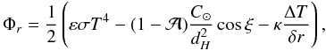 (7)with T [K] the temperature at the surface point for which the thermal balance is computed, and ΔT the temperature difference across the surface layer. This thermal balance is computed simultaneously for each point of the 2D grid to obtain the surface temperature distribution Tsurf(θ,ϕ).
This is then expanded on the basis of spherical harmonics, and the coefficients  of this expansion are used as the boundary conditions for Eq. (5):
 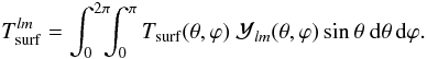 (8)We used the sampling theorem developed by Driscoll & Healy (1994) to derive these coefficients from the equilibrium temperature of the surface. Denoting N the number of points on one direction of the equally sampled surface grid, the boundary conditions
  are computed as
 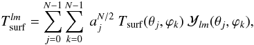 (9)with
  ,
,  the grid points coordinates,
  a coefficient that accounts for the over-sampling near the poles, and Tsurf [K] the equilibrium temperature at each point on the surface. The number of points N in one angular direction is determined by the heliocentric distance of the object (large number of samples for close objects to minimize the discretization errors) and the computational load (see Sect. 4.1).
In the center, the boundary condition is simpler and only depends on r: 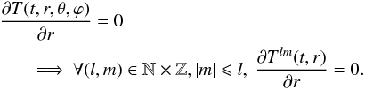 (10)\arraycolsep1.75ptThe (lmax + 1)2 Eq. (5) of Tlm are thus coupled by the use of these boundary conditions.
2.3. Heat sources
Experimental work by Schmitt et al. (1989) and subsequent cometary simulations have recognized crystallization of water ice as a major contributor to the activity of cometary bodies. Recent work by Jewitt (2009) on active Centaurs suggests that the crystallization of water ice may be the main driver of their activity. This heat source is described by  (11)with ϱa [kg m-3] the amorphous water ice bulk density. The phase transition releases a latent heat Hac = 9 × 10⁴ J kg-1 (Klinger 1981) at a rate from Schmitt et al. (1989):
  (12)Heat released upon decay of radioactive isotopes such as
  Al have long been recognized as an important heat source for solar system bodies (Urey 1955). We consider several short- and long-lived isotopes in this model (Table 1, values adapted from Castillo-Rogez et al. 2007, and ref. therein), commonly used in the thermal modeling of icy objects in the solar system. We consider two other short-lived radioactive isotopes than 26Al − 60Fe and 53Mn − with the aim of evaluating their influence on the initial differentiation. These internal heat sources can be described by
  (13)with ϱd the dust bulk density [kg m-3], Xrad the initial mass fraction of a considered isotope in the dust, Hrad [J kg-1] the heat released per unit mass upon decay, τrad [s] the decay time (see Table 1), and t the time.
Physical parameters of short-period (SP) and long-period (LP) radioactive isotopes considered in the model.
The initial abundance of radioactive isotopes is crucial for evaluating the thermal evolution of TNOs and Centaurs. The presence of these radioactive isotopes in the protoplanetary disk is constrained by the abundances of daughter isotopes contained in meteoritic material such as CAIs or chondrites. In particular, the presence of short-lived  Fe is deduced from the presence of Ni, and its abundance has not been well constrained yet (Gounelle & Meibom 2008). We thus have two limit values for its mass fraction, which are subject to modifications as more accuracy is applied to our knowledge of the
  Fe/Fe ratio (Gounelle et al. 2009).
The heat source term  also has to be expanded on the basis of spherical harmonics. As dust is assumed to be homogeneously distributed within the icy matrix, the heat released upon radioactive decay should also be homogeneous in the body. We also assume that crystallization is a phenomenon that depends only on r because of the homogeneous material distribution in each layer (see Sect. 3.3). Therefore, only depends on t and r, and the expansion gives
  (14)where δl,0 and δm,0 are Kronecker functions. These should be applied in Eq. (5).
3. Physical parameters relevant to TNOs
3.1. Bulk composition, heat capacity, and thermal conductivity
TNOs and Centaurs are generally assumed to have a comet-like composition thanks to the dynamical link between those populations (for a review see Coradini et al. 2008, and ref. therein). The relative mass fractions of water ice and dust should therefore be about 1:1 (Huebner et al. 2006). Nonetheless, TNOs display a wider range of densities than comets, from less than 1 g cm-3 to more than 2 g cm-3 (Sheppard et al. 2008), while cometary densities rarely exceed 1 g cm-3 (Blum et al. 2006), implying a wider range of porosity in TNOs compared to comet nuclei. The bulk density of comets, TNOs, and Centaurs is related to the porosity of the solid matrix ψ by the following equation:  (15)with XH2O and Xd the mass fractions of water ice and dust, respectively, and ρH2O and ρd [kg m-3] the densities of water ice and dust respectively.
The heat capacity of the mixture is obtained by computing the average of the values weighted by the mass fraction of each component:  (16)with XH2O and Xd the mass fraction of water ice and dust, and cH2O and cd [J kg-1 K-1] the heat capacities of each component. The numerical values used in this work can be found in Table 2.
Heat capacities and thermal conductivities.
The evaluation of the mixture thermal conductivity κ [W m-1 K-1] is difficult, since it depends on the material structure, the very different nature of components, and the porosity. However, we can assume that its value should be intermediate between the thermal conductivity of all components and that it should depend on the volume fraction of each. We also know that the porosity and granularity of the medium reduce the thermal conductivity, but it is unclear how and to what extent. We therefore consider the material as made of two phases, the pores and the solid matrix. The solid matrix thermal conductivity κs is computed as an average of each component’s thermal conductivity (see Table 2), weighted by its volume fraction: ![Mathematical equation: \begin{equation} \kappa _{\rm s} = x_{\rm H_2O} \left[(1-X_{\rm cr}) \kappa _{\rm a}+X_{\rm cr} \kappa _{\rm cr} \right]+x_{\rm d} \kappa _{\rm d}, \end{equation}](/articles/aa/full_html/2011/05/aa14194-10/aa14194-10-eq121.png) (17)with xH2O and xd the volume fractions of water ice and dust, respectively, and Xcr the mass fraction of crystalline water ice.
(17)with xH2O and xd the volume fractions of water ice and dust, respectively, and Xcr the mass fraction of crystalline water ice.
Within the empty pores the heat is transferred through thermal radiation:  (18)with rp the average pore radius taken as 1 μm, ε the medium emissivity, σ the Stefan-Boltzmann constant, and T the temperature in K (Huebner et al. 2006). The pores should be about the same size as the icy grains for a mean density of 500 kg m-3 (Huebner et al. 2006). We consider then the Hertz factor h, which is a correction factor to account for the granular structure of the solid. It should be applied to κs before correcting for the effects of porosity. Its value can vary from 10-4 to 1 (Huebner et al. 2006) due to sintering: we choose a constant value of 0.1, typically used for the simulation of comet thermal evolution (e.g. Huebner et al. 2006).
Finally, Shoshany et al. (2002) show that κp becomes predominant only for high values of the porosity (ψ > 0.7), so that generally κp ≪ κs. In this case, we can use the Russel formula (Russel 1935) to calculate a correction factor φ that should be applied to κs, to account for the effects of porosity (Espinasse et al. 1991; Coradini et al. 1997; Orosei et al. 1999). It depends on the porosity ψ, and the ratio  :
:  (19)Finally, the material effective thermal conductivity is
  (20)
(20)
3.2. Initial values
We define a nominal object with generic parameters found in Table 3. Some parameters can be directly derived from observations (radius, orbit, rotation period, etc.). We use average values for these parameters. Physical parameters related to the material (mass fractions, porosity, heat capacity, thermal conductivity, etc.) are difficult to infer from observations, so they are calculated using assumptions that were outlined in the previous section.
The bulk composition is a critical parameter when it comes to the thermal evolution of bodies such as TNOs and Centaurs. The amount of radionuclides is indeed directly linked to the dust mass fraction within the ice matrix. Figure 1 illustrates the central temperature evolution for the nominal object, using different dust mass fractions with a fixed porosity. This shows that ice-rich bodies (ρbulk = 830 kg m-3 in Fig. 1) tend to stay primitive, whereas ice-poor bodies (ρbulk = 1330 kg m-3 in Fig. 1) can be highly differentiated with internal temperatures exceeding 200 K.
Generic physical and orbital parameters considered for the nominal object.
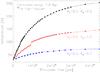 |
Fig. 1 Evolution of the central temperature as a function of simulated time for various compositions of the nominal object. Dust mass fractions: 30% (triangles), 50% (circles), and 70% (squares), with a fixed porosity. |
The choice of thermal conductivity is critical, since it affects the efficiency of thermal processes. Considering the thermal conductivity expression we used, the various values of porosity we tested appear to have little effect on the value of κ, and thus on the temperature distribution. The Hertz factor, on the other hand, makes the thermal conductivity vary much more and strongly influence the temperature as shown in Fig. 2 for the nominal object. High values of the thermal conductivity (high values of h) induce a more efficient cooling of the mixture. We considered a fixed value for the Hertz factor, although sintering makes it vary with temperature: when the internal temperature increases, the Hertz factor may also increase. The cooling would therefore be more effective with increasing temperature if we had accounted for sintering.
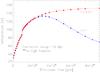 |
Fig. 2 Evolution of the central temperature as a function of simulated time for the nominal object, and different Hertz factors: h = 1 and h = 0.01, leading to κ = 6 × 10⁻¹ W m-1 K-1 and 6 × 10⁻³ W m-1 K-1, respectively. A formation delay of 1 Myr and the highest mass fraction of |
The object’s formation delay (time for the object to grow to its final size) is accounted for in the model through the decay of radioactive isotopes that occurs during accretion. This results in a decrease in each isotope’s abundance: 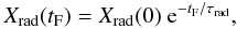 (21)with tF [s] the considered formation time, and Xrad(0) and τrad found in Table 1. We tested several delays, by considering a formation time of 1 Myr for the nominal object, and show results for a formation delay of 0 and 2 Myr. The formation time of TNOs and Centaurs is not well understood yet. Nonetheless, Weidenschilling (2004) suggests that 50 km-radius bodies could have been formed in less than one million years below 30 AU. Recent simulations from Kenyon et al. (2008) suggest that objects with a 1000 km-radius could be accreted in 5 to 10 × 106 years in the 20 − 25 AU region.
We assume that the objects undergo a cold accretion: they are formed from smaller planetesimals that cannot efficiently retain the internally produced heat (Prialnik & Podolak 1999). Therefore, accretional heating is neglected in this model. Accumulation of gravitational potential energy is generally assumed to be negligible even for large bodies such as Pluto (McKinnon et al. 1997), so we also neglect it here. During this formation period, it is therefore assumed that bodies do not suffer from much thermal modification (Sarid & Prialnik 2009), and an initial temperature of 30 K is reasonable. Since the formation period has not yet been fully constrained, its influence should be studied in detail.
The thermal emissivity ε of comet nuclei in the infrared is poorly constrained, but Hage & Greenberg (1990) showed that an aggregate of cometary grains could have a thermal emissivity close to 1, so we chose to use a generic value of 0.9 in our model. TNOs and Centaurs geometric albedos are usually very low (Stansberry et al. 2008) due to the processing of the surface by irradiation. We chose a Bond albedo of 10% for the nominal object. The corresponding geometric albedo stands in the 20%-range. While this might be high, the effect is actually very weak for TNOs, since insolation is not the dominant heat source.
3.3. Stratification
The temperature is computed for each point of the 3D-(r, θ, ϕ) grid. Physical parameters, such as c, κ, Xcr/Xam, and thus ρbulk, are temperature dependent, and therefore should be computed at each numerical iteration for every point on the 3D grid. Nonetheless, we limit the mathematical solution of Eq. (5), described by spherical harmonics functions, to spherical bodies with isotropic physical parameters. Within each shell – described by its radius r and its thickness Δr – the material properties are assumed to be homogeneous, even if the temperature is actually computed by accounting for its variations with the angular position. We consider one shell per point on the r-grid, and the distance between two grid points determines the thickness of each shell. The physical parameters inside each shell are thus defined using an average over θ and ϕ:  (22)with X any of the concerned physical parameters c, κ, and ρbulk through its dependency on Xam and Xcr, the mass fractions of amorphous and crystalline water ice, respectively. This might also introduce potentially large errors in the determination of the temperature distribution. We compared our results with a 1D model (Capria et al. 1996) to evaluate the error made with the stratification assumption. For objects like TNOs, it has been found to be negligible (temperature differences less than 1%).
Objects closer to the Sun are potentially subject to heterogeneous differentiation (in particular crystallization) due to insolation. In this case, using averaged parameters instead of the real parameters might induce larger errors since these are temperature-dependent. Our simulations have shown that the error on the temperature distribution is limited to a few Kelvins, 10 K at most for objects with perihelion distances greater than 5 AU. Larger errors (10 − 20%) are nonetheless encountered closer to the Sun, particularly for heliocentric distance below 5 AU. Therefore, this model in its current form is not suitable for objects reaching small heliocentric distances like comets. Improvements in the treatment of physical parameters should be applied to reduce the error.
4. Validation
4.1. Mathematical approximation
The most critical approximation we make is related to the expansion of temperature into the basis of spherical harmonics. This expansion is exact as long as the degree l goes to infinity. For numerical reasons we have to truncate the sum (4) to a maximum degree lmax. We thus introduce an error that should be kept as small as possible, by considering both a high lmax and a tight sampling of the surface temperature distribution at the same time. Indeed, a sampling theorem only gives a perfect reconstruction for band-limited functions, which our surface temperature distribution is not. Therefore, we have to make sure that the sampling is tight enough to obtain a good approximation of the surface temperature.
The case of lmax = 0 corresponds to the homogeneous solution (with homogeneous heating and cooling), which can be achieved at an infinite heliocentric distance. The degree lmax has to be increased as the heliocentric distance decreases, i.e. when the solar illumination becomes a predominant heat input, inducing strong variations of the boundary condition with the angular position on the surface. At the same time, the number of samples at the surface needs to increase, and it is indeed useless to consider a high maximum degree for a few samples, because it is useless to consider a large number of samples at the surface if the maximum degree is low. Increasing lmax and the sampling increases not only numerical accuracy but also the numerical cost. In an attempt to find a compromise between the two, we performed simulations aimed at finding a suitable cutoff-value for different heliocentric distances.
Our simulations have shown that for a TNO (heliocentric distance over 30 AU), the coefficients Tlm(t,r) have a negligible value for l larger than 7: the contribution of the respective spherical harmonics becomes negligible in the sum over all degrees. This case corresponds to a sampling of 17 × 16 points of the surface (θ,ϕ)-grid. For Centaurs, which are closer to the Sun, the maximum degree should be about 15 to assure a negligible contribution of all spherical harmonics actually truncated. This is the case for a sampling of 33 × 32 points of the surface (θ,ϕ)-grid. The temperature variations due to the choice of lmax above this value are then limited to less than 1%. This means that increasing the value of lmax and the number of samples does not induce any noticeable change in the temperature distribution. It is, however, recommended to increase these two parameters when the simulations are run to model a long period of time, in order to avoid large truncation errors.
4.2. Comparison with another 3D model
We carefully compared this model (3DSH in this section) with the 3D model developed by Rosenberg & Prialnik (2007) (3DRos in this section). The models differ both in the mathematical and the numerical formulation of the physical processes. In the 3Dros model, the differential equation is transformed into a set of difference equations, applied to a 3D-(r, θ, ϕ) grid. The temperature is directly determined for each point on the grid, through a fully implicit scheme. For the comparison, we considered an object with initial parameters summarized in Table 4. We considered an object closer to the Sun than a TNO, so as to obtain more thermal input from insolation. We ran the two models with the same parameters for several orbits, and compared the results especially at the surface, where insolation induces 2D-(θ, ϕ) variations in the temperature. The same 3D grid was used to make this comparison. The surface temperature found with our model (3DSH) is illustrated in the top panel in Fig. 3.
Physical and orbital parameters used for the comparison of the two 3D models.
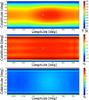 |
Fig. 3 Top: temperature distribution at the surface of comparison object determined with the 3DSH model. Middle: fractional difference between the 3DSH model and the 3DRos model using low resolution at the surface. Bottom: fractional difference between the 3DSH model and the 3DRos model using a higher resolution at the surface. White diamonds indicate the position of the subsolar point. |
We evaluated the relative difference between the two models by making the following operation: δ = (3DSH – 3DRos)/3DSH (see middle and bottom panels of Fig. 3). We first used a sampling with a few points (17 × 16 points) at the surface, although the small heliocentric distance would require a tighter sampling. The corresponding relative difference δ is displayed in the middle panel of Fig. 3. It shows that although the results are in excellent agreement for most of the surface, an important difference is produced at the poles of the object. The maximum relative difference is 14%. The discrepancy at the poles can be due to several factors. First the temperature at the poles is not directly computed in the 3DRos model, but extrapolated. The lower confidence colatitudes are below 5 deg and over 175 deg. In the 3DSH model, two factors could be implied: 1) the use of spherical harmonics for our boundary condition at the surface, which is not a band-limited function, and thus requires using as tight a sampling as possible; and 2) the discontinuity produced at the poles by the use of the sampling theorem (factor sinθ in the coefficient aj). The maximum relative difference is reduced to a few percent when colatitudes smaller than 5 deg and larger than 175 deg are excluded (Table 5).
Numerical results from the comparison between the 3DRos and the 3DSH (two surface samplings) models.
We then considered tighter samplings. The bottom panel of Fig. 3 shows the relative difference for 65 × 64 samples at the surface. In this case, the maximum relative difference is 6%, which is reduced to 2% when the polar regions are excluded from the calculation. This comparison illustrates how important the sampling can be for objects close to the Sun in order to reach maximum accuracy in the 3DSH model. Again, the case of lmax = 0 corresponds to a homogeneous solution achieved at an infinite heliocentric distance. The degree lmax has to be increased as the heliocentric distance decreases, the number of samples at the surface needs to increase at the same time (see previous section).
The few percent span that we find is nonetheless excellent considering the very different mathematical and numerical formulations of the physical processes in both models. Used in the same conditions (same sampling mainly), the 3DSH model is about 10 times faster (12 h vs. 155 h for the 17 × 16 sampling).
4.3. Early evolution of TNOs: comparison with other models
Although focused on the volatile content of TNOs, studies performed by DeSanctis et al. (2001) and Choi et al. (2002) show that their composition could be altered by early heating due to the decay of short-lived radioactive isotopes, to result in a layered structure. They find that undifferentiated cores could survive, though, depending on the amount of isotopes within the dust. Choi et al. (2002) suggest that an amorphous layer as thick as 40 km could survive at the surface of the objects. The heliocentric distance appeared to have little influence on this early stage of the evolution.
We confirm that the internal structure that results from the heating by short-lived radioactive isotopes can be very diverse, from completely primitive to strongly differentiated. The amount of radionuclides is crucial, as suggested by Choi et al. (2002) and illustrated by Figs. 4 and 5. Figure 4 shows the variations in the internal temperature due to the poor constrain on the initial mass fraction of isotopes. Figure 5 shows the variations in the internal temperature due to isotope’s abundance decrease during the formation delay, i.e. time for the objects to grow to their final radii. We find that the error on the initial mass fraction of Fe can induce a variation of up to 40 K in the internal temperature. We also find that, if the nominal body is formed rapidly (less than 0.5 Myr), it should experience a physical differentiation, including melting of water ice in the inner parts. For all formation delays greater than 2.0 Myr, the nominal body can preserve its initial structure due to low thermal modification. For a formation delay of 1.0 Myr, all objects with a radius larger than 10 km should be differentiated, at least from a chemical point of view, i.e. crystallization of water ice, inducing release of trapped volatiles.
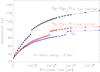 |
Fig. 4 Evolution of the central temperature as a function of simulated time for the nominal object and a formation delay of 1.0 Myr years, considering various fractions of short-lived radiogenic elements: |

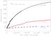 |
Fig. 5 Evolution of the central temperature for the nominal object, considering different formation delays −2.0 Myr (squares), 1.0 Myr (triangles), and 0.0 Myr (circles)–, as a function of the simulated time. High-mass fraction of short-lived radiogenic element |
A way to change these time constraints would be to consider a different density, to account for other physical processes, or to account for the presence of salt or other material that can lower the melting point (see Desch et al. 2009). In addition, these results were found using the cold accretion assumption and by neglecting both accretional heating and gravitational potential energy. This assumption might be valid only for objects forming far from the Sun, in regions where relative velocities are low and dynamical timescales long. Accounting for the accretional heating could increase the thermal modifications of objects formed closer to the Sun, where relative velocities and dynamical timescales are important, as shown by Merk & Prialnik (2006).
5. Amorphous vs. crystalline water ice on the surface of TNOs
5.1. Observations and laboratory experiments
Observations of TNOs and Centaurs have revealed the presence of water ice on their surfaces, through the presence of two absorption bands located 1.5 and 2.0 μm in some spectra (Barkume et al. 2008; Guilbert et al. 2009). In addition to these bands, a feature at 1.65 μm is generally used to diagnose the presence of crystalline water ice. This band is observed in the spectra of largest objects (see Barucci et al. 2008b, and ref. therein). Observations suggest that objects with diameters larger than about 700 km that show water ice bands in their spectra should also show the 1.65 μm band, thus indicating the presence of crystalline water ice. The case of smaller objects could be more controversial, since the observations are very miscellaneous. Some spectra show the 1.5 and 2.0 μm features, with or without the additional crystalline water ice absorption band, while some others do not show any features. Nonetheless, there is a strong observational bias concerning any detection of features on small objects’ spectra, since these would generally have signal-to-noise ratios that are inadequate for determining the presence of any absorption band accurately.
Spectral modeling using radiative transfer models has suggested that amorphous water ice should be added to the geographical and intimate mixtures in order to obtain a better fit of these spectra, even when a 1.65 μm feature is observed (Merlin et al. 2007). It is thus expected that both amorphous and crystalline water ice should be present on the surface of TNOs and Centaurs, even though there is still no direct evidence of amorphous ice. In addition, spectral modeling results are not unique and depend on the quality of the optical constants, the mixture are chosen according to our a priori knowledge of the objects.
Finally, we caution that the inferred presence of crystalline water ice is hard to reconcile with results from laboratory studies by Strazzulla & Palumbo (1998) that indicate that water ice is amorphized by space weathering on short timescales. Some experiments have shown that – depending on the temperature – it is very difficult from a spectral point of view to distinguish between amorphous water ice and amorphized crystalline water ice. Even when crystalline water ice is amorphized, a 1.65 μm feature can remain (Mastrapa & Brown 2006; Zheng et al. 2009). As a consequence, it is still very difficult to determine whether crystalline water ice is actually present or not on the surface of TNOs and Centaurs. No experiment has been undertaken so far to understand whether the 1.65 μm band could be produced by irradiation of amorphous ice, and Cook et al. (2007) show that there should not be any process responsible for producting crystalline water ice at the typical TNOs heliocentric distances, except for the internal heating. We can thus assume that the presence of the 1.65 μm band in TNOs spectra indicates at least that there once was crystalline water ice on their surfaces.
5.2. Amorphous surface layer
Despite the internal heating due to radioactive decay, the surface of TNOs is in thermal equilibrium. At the heliocentric distance considered for the simulations, the surface temperature is about 45 − 50 K at most. This prevents the heat wave from reaching the surface. In other words, a cold wave propagates from the surface toward deeper layers. The competition between the heat and cold waves is thus responsible for conserving an amorphous water-ice layer at the surface. Choi et al. (2002) find that water ice could stay amorphous up to 40 km below the surface. Prialnik et al. (2008) find that about 20 km of a surface layer could stay pristine.
We find that, when the thermal evolution is dominated by short-lived isotopes decay, the thickness of the amorphous layer strongly depends on the objects size, as well as on the formation delay. For small initial amounts of radioactive nuclides, the crystallization process is less effective, because the layer is thus thicker. Bigger objects retain a thinner layer, as shown on Table 6, considering a formation delay of 1 Myr (maximum thickness is achieved with the lowest mass fraction of Fe, minimum thickness is obtained with its higher mass fraction). However, objects formed close enough to the Sun for the surface temperature to reach the crystallization threshold do not maintain this amorphous surface layer. They can nonetheless maintain an amorphous sub-surface layer squeezed between the crystalline deeper layers and the surface crystalline layer. The size scales involved are small enough for collisions to erode the surfaces efficiently enough to let the crystalline water ice underneath the surface appear and contribute to the overall spectra.
Thickness of the amorphous water ice layer on the surface, for various objects’ radii.
When the thermal evolution is dominated by the decay of long-lived isotopes decay, the thickness of the amorphous layer preserved at the surface is almost independent of the object’s size, and the largest objects still have a large amorphous surface layer after 4.6 Gyr of thermal evolution. Although McKinnon et al. (2008) find that objects with radii larger than 75 km can suffer from substantial crystallization, we find that the process is barely initiated in the central parts of an object with the nominal composition and a 100 km radius (Fig. 6). For objects with a larger radius, crystallization is triggered, and only a surface layer of 20 to 40 km thick (depending on the object’s size) remains amorphous. This confirms the size range found by Prialnik et al. (2008) (20 km) and Choi et al. (2002) (40 km).
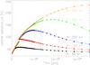 |
Fig. 6 Evolution of the central temperature for objects with the nominal composition under the effect of long-lived isotopes decay. Several radii are shown: 50 km (black squares), 100 km (red diamonds), 200 km (blue upward triangles), 300 km (green downward triangles), and 500 km (orange dots). |
We also find that, although large objects with a cometary composition can suffer from chemical differentiation, their internal temperatures do not allow for the water ice to melt. This would require the presence of compounds that can lower the mixture melting point or require different mixture thermal properties. Indeed, the density (which influence the amount of nuclides) and the thermal conductivity appear to be key parameters when it comes to the thermal evolution of TNOs over the age of the solar system. Decreasing the value of the thermal conductivity induces a slow propagation of the cold wave inside the body, and the internal temperatures can reach higher values. (We considered h = 0.01 to reduce the thermal conductivity.) The surface amorphous layer is thus thinner, about 10 km. Increasing the density of the objects obviously increases the dust content of the material. It thus induces a more efficient heating of the bodies. For instance, if we consider a density of 1710 kg m-3, a 300 km-radius body would suffer from a physical differentiation (presence of liquid water, see Fig. 7). Finally, when considering both a higher density and a lower thermal conductivity, the bodies suffer from more efficient heating and less efficient cooling. In this case the thickness of the surface amorphous layer is only a few kilometers and can be efficiently eroded by collisions.
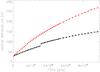 |
Fig. 7 Evolution of the central temperature for an object with a 300 km radius and different densities: 1020 kg m-3 (black squares) and 1710 kg m-3 (red dots). The other parameters are those of the nominal object. The heat source is the decay of long-lived radionuclides. |
5.3. Discussion
Simulations of the thermal evolution of TNOs and Centaurs suggest that, if the water ice was initially crystalline, it would have stayed so in the internal parts of the bodies. Only the surface would have been amorphized by space weathering. However, partial cratering of the surface could bring the underlying crystalline water ice to the surface, so that it would contribute to the overall spectrum.
If water ice was initially amorphous, simulations performed by various groups suggest that a layer of amorphous water ice would be maintained at the surface of the objects, provided they are formed far enough from the Sun (10 − 15 AU) to prevent any crystallization from insolation. Short-lived isotope decay provides an efficient heating of the bodies, but the objects need to be formed rapidly to benefit from this powerful heat source. Regardless of the effects of the short-lived nuclides, long-lived nuclides would heat the bodies later during the evolution. When the internal structure is dominated by the early radioactive heating, the thickness of the amorphous layer depends on the object’s size and formation delay (time for it to grow to its final size). For objects that can actually suffer from crystallization, this results in a thin layer that can be easily removed by impact cratering, so as to reveal the crystalline water ice underneath.
When the thermal evolution is dominated by the effects of long-lived radionuclides, the thickness of the amorphous layer on the surface depends mainly on the thermal conduction and the density of the objects. The simulations suggest that the layer can be very thick, and thus should not be eroded efficiently by impacts. Nonetheless, a higher density and a lower thermal conductivity would allow the largest objects (radius larger than about 300 km) to retain a thin pristine layer and even suffer from a physical differentiation.
Therefore, our results suggest that small TNOs should stay primitive unless 1) they were formed quickly; 2) they are debris from the disruption of larger bodies; and 3) they were formed close enough to the Sun (10 − 15 AU) for crystallization to be triggered at the surface by insolation. The presence of crystalline water ice at the surface of larger objects could be due to
-
1)
rapid formation;
-
2)
formation close to the Sun for crystallization to be triggered by insolation;
-
3)
a high density, which is actually observed for the large objects (Brown 2008);
-
4)
low thermal conductivity, especially close to the surface, which could actually be the case (results from measurements, see for example Groussin et al. 2004);
-
5)
a combination of several of these parameters.
Considering these possibilities, and not accounting for the production of crystalline water ice by some other process, we suggest that objects larger than about 300 km with densities of at least 1500 kg m-3 would present some crystalline water ice on their surface. Crystalline water ice might be produced from amorphous water ice in the subsurface layers, or could come from the presence of liquid water in the internal parts that could then propagate toward the surface through cracks. If the thermal conductivity of the surface layers is additionally very low, the presence of crystalline water ice could simply be due to the erosion of the surface by impact cratering, revealing the underlying material. These conclusions highlight the importance of objects like Quaoar (ρbulk > 2800 kg m-3, Fraser & Brown 2009) or Orcus (ρbulk = 1500−1900 kg m-3, Brown 2008; Brown et al. 2010), which are intermediate both in sizes and densities. Their thermal evolutions might be complex and would require detailed studies (see Desch et al. 2009; Delsanti et al. 2010, for example).
6. Conclusions
We have developed a new 3D thermal evolution model. The main asset of this model is to account for lateral heat fluxes, which allow us to achieve a realistic description of thermal processes, especially on the surface, where insolation induces temperature variations with angular position. We compared this model to a 1D model and obtained results similar to those shown by Orosei et al. (1999). The pole’s temperature does not decrease over time as in 1D results, since heat is diffused from the equator toward the poles. The comparison between the temperature evolutions obtained with this new model and with the 3D model presented by Rosenberg & Prialnik (2007) also shows excellent agreement. Used in the same conditions, this new model is about ten times faster.
Although this model in its current form is not as sophisticated as 1D models from a physical point of view, it opens a wide range of possible studies: heterogeneities of albedo at the surface, for example. Some improvements will be made in the future, to account for variations of physical parameters, such as porosity or composition with the depth, and to allow angular variations of the composition within each layer. Some volatile compounds could also be added, and their sublimation should also be accounted for. This new model uses a fast algorithm that opens the possibility for many improvements, such as introducing of new physical processes or heterogeneities in material properties, that reach the level of physical sophistication of current 1D models.
The comparison of results for the early thermal evolution of TNOs obtained with this model and others show excellent agreement. We indeed confirmed that classical Kuiper Belt objects could have remained primitive, whereas scattered disk objects and Oort cloud objects could be more differentiated. We also tried to interpret the presence/absence of crystalline water ice at the surface of TNOs. We find that unless the objects are formed rapidly, the thermal evolution is dominated by the decay of long-lived isotopes. In this case, only large objects (R > 300 km) with a density of at least 1500 kg m-3 should contain crystalline water ice close to the surface. We also find that intermediate objects (diameters ranging from 500 to 1000 km) should be an interesting population, deserving detailed observational and modeling studies, since these objects would be at the transition, both in sizes and densities, between differentiated and primitive bodies.
Acknowledgments
A.G.L. thanks G. Magni, M. T. Capria, M. C. De Sanctis and D. Turini for useful discussions on the model, and D. Jewitt for useful comments on the manuscript. J.L. thanks the LPI contribution 1549. A.G.L. was supported in part by a NASA Herschel grant to David Jewitt. The authors want to thank the anonymous referee for their useful comments that contributed to a major improvement of the manuscript.
References
- Barkume, K. M., Brown, M. E., & Schaller, E. L. 2008, AJ, 135, 55 [NASA ADS] [CrossRef] [Google Scholar]
- Barucci, M. A., Boehnhardt, H., Cruikshank, D. P., et al. 2008a, in The Solar System Beyond Neptune, ed. M. A. Barucci, H. Boehnhardt, D. Cruikshank, & A. Morbidelli (Tucson: University of Arizona Press), 592, 3 [Google Scholar]
- Barucci, M. A., Brown, M. E., Emery, J. P., et al. 2008b, in The Solar System Beyond Neptune, ed. M. A. Barucci, H. Boehnhardt, D. Cruikshank, & A. Morbidelli (Tucson: University of Arizona Press), 592, 143 [Google Scholar]
- Barucci, M. A., Merlin, F., Guilbert, A., et al. 2008c, A&A, 479, 13 [NASA ADS] [CrossRef] [EDP Sciences] [Google Scholar]
- Belton, M. J. S., & Melosh, J. 2009, Icarus, 200, 280 [Google Scholar]
- Blum, J., Schräpler, R., Davidsson, B. J. R., et al. 2006, ApJ, 652, 1768 [NASA ADS] [CrossRef] [Google Scholar]
- Brown, M. E. 2008, in The Solar System Beyond Neptune, ed. M. A. Barucci, H. Boehnhardt, D. P. Cruikshank, & A. Morbidelli (Tucson: University of Arizona Press), 592, 335 [Google Scholar]
- Brown, M. E., Ragozzine, D., Stansberry, J., et al. 2010, AJ, 139, 2700 [CrossRef] [Google Scholar]
- Brunetto, R., & Roush, T. L. 2008, A&A, 481, 879 [NASA ADS] [CrossRef] [EDP Sciences] [Google Scholar]
- Capria, M. T., Capaccioni, F., Coradini, A., et al. 1996, Planet. Space Sci., 44, 987 [Google Scholar]
- Castillo-Rogez, J. C., Matson, D. L., Sotin, C., et al. 2007, Icarus, 190, 179 [NASA ADS] [CrossRef] [Google Scholar]
- Choi, Y., Cohen, M., Merk, R., et al. 2002, Icarus, 160, 300 [NASA ADS] [CrossRef] [Google Scholar]
- Cohen, M., Prialnik, D., & Podolak, M. 2003, New A, 8, 179 [Google Scholar]
- Cook, J. C., Desch, S. J., Roush, T. L., et al. 2007, ApJ, 663, 1406 [NASA ADS] [CrossRef] [Google Scholar]
- Coradini, A., Capaccioni, F., Capria, M. T., et al. 1997, Icarus, 129, 317 [NASA ADS] [CrossRef] [Google Scholar]
- Coradini, A., Capria, M. T., DeSanctis, M. C., et al. 2008, in The Solar System Beyond Neptune, ed. M. A. Barucci, H. Boehnhardt, D. Cruikshank, & A. Morbidelli (Tucson: University of Arizona Press), 592, 243 [Google Scholar]
- Delsanti, A., Merlin, F., & Guilbert-Lepoutre, A. 2010, A&A, 520, A40 [NASA ADS] [CrossRef] [EDP Sciences] [Google Scholar]
- DeSanctis, M. C., Capria, M. T., & Coradini, A. 2001, AJ, 121, 2792 [NASA ADS] [CrossRef] [Google Scholar]
- Desch, S. J., Cook, J. C., Dogget, T. C., et al. 2009, Icarus, 202, 694 [NASA ADS] [CrossRef] [Google Scholar]
- Doressoundiram, A., Boehnhardt, H., Tegler, S. C., et al. 2008, in The Solar System Beyond Neptune, ed. M. A. Barucci, H. Boehnhardt, D. Cruikshank, & A. Morbidelli (Tucson: University of Arizona Press), 592, 91 [Google Scholar]
- Driscoll, J. R., & Healy, D. M. 1994, Adv. in Applied Math., 15, 202 [Google Scholar]
- Duncan, M. J., & Levison, H. F. 1997, Science, 276, 1670 [NASA ADS] [CrossRef] [PubMed] [Google Scholar]
- Ellsworth, K., & Schubert, G. 1983, Icarus, 54, 490 [NASA ADS] [CrossRef] [Google Scholar]
- Enzian, A., Cabot, H., & Klinger, J. 1997, A&A, 319, 995 [NASA ADS] [Google Scholar]
- Espinasse, S., Klinger, J., Ritz, C., et al. 1991, Icarus, 92, 350 [NASA ADS] [CrossRef] [EDP Sciences] [Google Scholar]
- Fanale, F. P., & Savail, J. R. 1984, Icarus, 60, 476 [NASA ADS] [CrossRef] [Google Scholar]
- Fraser, W., & Brown, M. E. 2009, AAS/Division for Planetary Sciences Meeting Abstracts, 41, 65.03 [Google Scholar]
- Giauque, W. F., & Stout, J. W. 1936, Am. Chem. Soc. J., 58, 1144 [Google Scholar]
- Gomes, R. 2003, Icarus, 161, 404 [Google Scholar]
- Gounelle, M., & Meibom, A. 2008, ApJ, 680, 781 [NASA ADS] [CrossRef] [Google Scholar]
- Gounelle, M., Meibom, A., Hennebelle, P., et al. 2009, ApJ, 694, 1 [Google Scholar]
- Groussin, O., Lamy, P., & Jorda, L. 2004, A&A, 413, 1163 [NASA ADS] [CrossRef] [EDP Sciences] [Google Scholar]
- Guilbert, A., Alvarez-Candal, A., Merlin, F., et al. 2009, Icarus, 201, 272 [NASA ADS] [CrossRef] [Google Scholar]
- Hage, J. I., & Greenberg, J. M. 1990, ApJ, 361, 251 [NASA ADS] [CrossRef] [Google Scholar]
- Hainaut, O. R., Delahode, C. E., Boehnhardt, H., et al. 2000, A&A, 356, 1076 [NASA ADS] [Google Scholar]
- Herman, G., & Podolak, M. 1985, Icarus, 61, 252 [NASA ADS] [CrossRef] [Google Scholar]
- Huebner, W. F., Benkhoff, J., Capria, M. T., et al. 2006, in Heat and gaz diffusion in comet nuclei, published for the Int. Sp. Sci. Inst., Bern, Switzerland (Noordwijk, The Netherlands: ESA publ. div.) [Google Scholar]
- Jewitt, D. 2009, AJ, 137, 4296 [NASA ADS] [CrossRef] [Google Scholar]
- Kenyon, S. J., Bromley, B. C., O’Brien, D. P., et al. 2008, in The Solar System Beyond Neptune, ed. M. A. Barucci, H. Boehnhardt, D. Cruikshank, & A. Morbidelli (Tucson: University of Arizona Press), 592, 293 [Google Scholar]
- Klinger, J. 1980, Science, 209, 271 [NASA ADS] [CrossRef] [PubMed] [Google Scholar]
- Klinger, J. 1981, Icarus, 47, 320 [NASA ADS] [CrossRef] [Google Scholar]
- Lasue, J., De Sanctis, M. C., Coradini, A., et al. 2008, Planet. Space Sci., 56, 1977 [NASA ADS] [CrossRef] [Google Scholar]
- Mastrapa, R. M. E., & Brown, R. H. 2006, Icarus, 183, 207 [NASA ADS] [CrossRef] [Google Scholar]
- McKinnon, W. B., Simonelli, D., & Schubert, G. 1997, in Pluto and Charon, ed. S. A. Stern, & D. J. Tholen (Tucson: Univ. of Arizona Press), 295 [Google Scholar]
- McKinnon, W. B., Prialnik, D., Stern, S. A., et al. 2008, in The Solar System Beyond Neptune, ed. M. A. Barucci, H. Boehnhardt, D. Cruikshank, & A. Morbidelli (Tucson: University of Arizona Press), 592, 213 [Google Scholar]
- Merk, R., & Prialnik, D. 2006, Icarus, 183, 283 [NASA ADS] [CrossRef] [Google Scholar]
- Merlin, F., Guilbert, A., Dumas, F., et al. 2007, A&A, 466, 1185 [NASA ADS] [CrossRef] [EDP Sciences] [Google Scholar]
- Noll, K. S., Grundy, W. M., Chiang, E. I., et al. 2008, in The Solar System Beyond Neptune, ed. M. A. Barucci, H. Boehnhardt, D. Cruikshank, & A. Morbidelli (Tucson: University of Arizona Press), 592, 345 [Google Scholar]
- Orosei, R., Capaccioni, F., Capria, M. T., et al. 1999, Planet. Space Sci., 47, 839 [NASA ADS] [CrossRef] [Google Scholar]
- Prialnik, D., & Podolak, M. 1999, Space Sci. Rev., 90, 169 [NASA ADS] [CrossRef] [Google Scholar]
- Prialnik, D., Sarid, G., Rosenberg, E., et al. 2008, Space Sci. Rev., 138, 147 [NASA ADS] [CrossRef] [Google Scholar]
- Rosenberg, E. D., & Prialnik, D. 2007, Astron., 12, 523 [Google Scholar]
- Russel 1935, J. Am. Ceram. Soc., 18, 1 [CrossRef] [Google Scholar]
- Sarid, G., & Prialnik, D. 2009, Met. & Plan. Sci., 44, 1905 [NASA ADS] [CrossRef] [Google Scholar]
- Schmitt, B., Espinasse, S., Grim, R. J. A., et al. 1989, Phys. and Mech. of Cometary Mat., 302, 65 [Google Scholar]
- Sheppard, S. S., Lacerda, P., & Ortiz, J. L. 2008, in The Solar System Beyond Neptune, ed. M. A. Barucci, H. Boehnhardt, D. Cruikshank, & A. Morbidelli (Tucson: University of Arizona Press), 592, 129 [Google Scholar]
- Shoshany, Y., Prialnik, D., & Podolak, M. 2002, Icarus, 157, 219 [NASA ADS] [CrossRef] [Google Scholar]
- Stansberry, J., Grundy, W., Brown, M., et al. 2008, in The Solar System Beyond Neptune, ed. M. A. Barucci, H. Boehnhardt, D. Cruikshank, & A. Morbidelli (Tucson: University of Arizona Press), 592, 161 [Google Scholar]
- Strazzulla, G., & Palumbo, M. E. 1998, Planet. Space Sci., 46, 1339 [Google Scholar]
- Strazzulla, G., Baratta, G. A., Johnson, R. E., et al. 1991, Icarus, 91, 101 [NASA ADS] [CrossRef] [Google Scholar]
- Tegler, S. C., Bauer; J. M., Romanishin, W., et al. 2008, in The Solar System Beyond Neptune, ed. M. A. Barucci, H. Boehnhardt, D. Cruikshank, & A. Morbidelli (Tucson: University of Arizona Press), 592, 105 [Google Scholar]
- Urey, H. C. 1955, Proc. Nat. Acad. Sci., 41, 127 [Google Scholar]
- Weidenschilling, S. J. 2004, in Comets II, ed. M. C. Festou, H. U. Keller, & H. A. Weaver (Tucson: University of Arizona Press), 745, 97 [Google Scholar]
- Wierczorek, M. A. 2007, Treatise on Geophysics, 10, 165 [Google Scholar]
- Zheng, W., Jewitt, D., & Kaiser, R. I. 2009, J. Phys. Chem., 113, 11174 [Google Scholar]
All Tables
Physical parameters of short-period (SP) and long-period (LP) radioactive isotopes considered in the model.
Numerical results from the comparison between the 3DRos and the 3DSH (two surface samplings) models.
Thickness of the amorphous water ice layer on the surface, for various objects’ radii.
All Figures
|
Fig. 1 Evolution of the central temperature as a function of simulated time for various compositions of the nominal object. Dust mass fractions: 30% (triangles), 50% (circles), and 70% (squares), with a fixed porosity. |
| In the text | |
|
Fig. 2 Evolution of the central temperature as a function of simulated time for the nominal object, and different Hertz factors: h = 1 and h = 0.01, leading to κ = 6 × 10⁻¹ W m-1 K-1 and 6 × 10⁻³ W m-1 K-1, respectively. A formation delay of 1 Myr and the highest mass fraction of |
| In the text | |
|
Fig. 3 Top: temperature distribution at the surface of comparison object determined with the 3DSH model. Middle: fractional difference between the 3DSH model and the 3DRos model using low resolution at the surface. Bottom: fractional difference between the 3DSH model and the 3DRos model using a higher resolution at the surface. White diamonds indicate the position of the subsolar point. |
| In the text | |
|
Fig. 4 Evolution of the central temperature as a function of simulated time for the nominal object and a formation delay of 1.0 Myr years, considering various fractions of short-lived radiogenic elements: |
| In the text | |
|
Fig. 5 Evolution of the central temperature for the nominal object, considering different formation delays −2.0 Myr (squares), 1.0 Myr (triangles), and 0.0 Myr (circles)–, as a function of the simulated time. High-mass fraction of short-lived radiogenic element |
| In the text | |
|
Fig. 6 Evolution of the central temperature for objects with the nominal composition under the effect of long-lived isotopes decay. Several radii are shown: 50 km (black squares), 100 km (red diamonds), 200 km (blue upward triangles), 300 km (green downward triangles), and 500 km (orange dots). |
| In the text | |
|
Fig. 7 Evolution of the central temperature for an object with a 300 km radius and different densities: 1020 kg m-3 (black squares) and 1710 kg m-3 (red dots). The other parameters are those of the nominal object. The heat source is the decay of long-lived radionuclides. |
| In the text | |
Current usage metrics show cumulative count of Article Views (full-text article views including HTML views, PDF and ePub downloads, according to the available data) and Abstracts Views on Vision4Press platform.
Data correspond to usage on the plateform after 2015. The current usage metrics is available 48-96 hours after online publication and is updated daily on week days.
Initial download of the metrics may take a while.