| Issue |
A&A
Volume 528, April 2011
|
|
|---|---|---|
| Article Number | L2 | |
| Number of page(s) | 4 | |
| Section | Letters | |
| DOI | https://doi.org/10.1051/0004-6361/201116488 | |
| Published online | 16 February 2011 | |
Letters to the Editor
Hadronic beam models for quasars and microquasars
1
ICREA & Institut de Ciències de l’Espai (IEEC-CSIC), Campus
UAB, Facultat de Ciències,
Torre C5-parell, 2a planta,
08193
Barcelona,
Spain
e-mail: This email address is being protected from spambots. You need JavaScript enabled to view it.
2
Institut für Theoretische Physik, and Institut für Astro- und
Teilchenphysik, Leopold-Franzens-Universität Innsbruck, Technikerstr. 25, 6020
Innsbruck,
Austria
Received:
10
January
2011
Accepted:
2
February
2011
Abstract
Context. Most of the hadronic jet models for quasars (QSOs) and microquasars (MQs) found in the literature represent beams of particles (e.g. protons). These particles interact with the matter in the stellar wind of the companion star in the system or with crossing clouds, generating γ-rays via proton-proton processes.
Aims. Our aim is to derive the particle distribution in the jet as seen by the observer, so that the γ-ray and neutrino yields can be properly computed.
Methods. We use relativistic invariants to obtain the transformed expressions in the cases of both a power law and power law with a cutoff particle distribution in the beam. We compare them with previous expressions used earlier in the literature.
Results. We show that formerly used expressions for the particle distributions in the beam as seen by the observer are in error, with the differences being strongly dependent on the viewing angle. For example, for Γ = 10 (Γis the Lorentz factor of the blob) and angles larger than ~20°, the calculation used earlier entails an overprediction (order of magnitude or more) of the proton spectra for E > Γmc2, whereas it always overpredicts (two orders of magnitude) the proton spectrum at lower energies, for all the viewing angles.
Conclusions. All the results for photon and neutrino fluxes in hadronic models are affected in beams that have made use of the earlier calculation. Given that correct γ-ray fluxes will in almost any case be significantly diminished in comparison with published results and that the time of observations in Cherenkov facilities grows with the square of the flux-reduction factor in a statistically limited result, the possibility of observing hadronic beams is undermined.
Key words: ISM: jets and outflows / astroparticle physics / Gamma rays: general
© ESO, 2011
1. Introduction
The study of the possible high-energy radiation from QSOs and MQs is uncertain in one central aspect, the particle composition of the jets. Is the radiation emitted produced mainly via inverse Compton (self-synchrotron and/or with external fields) or via proton-proton/proton-photon interactions leading to subsequent meson decay? In the latter case, hadronic jet models have been used to assess this possibility. Most of these models represent beams of particles (e.g. protons) linearly propagating in a direction normal to an accretion disk, interacting with the matter in the stellar wind of the companion star in the case of MQs or with matter in clouds in the case of quasars. The protons in the beams are usually assumed to be distributed with a power law that may be cut at high energies, as is the case when they were accelerated in Fermi processes within the jet and subject to losses. It is then crucial to have a correct description of the proton distribution as seen by the observer, since the emissivity of γ-rays and neutrinos produced by charged and neutral pions make use of the cross sections known in that frame. In this paper we present the derivation of a beam particle distribution as seen by the observer and compare it with the expression used earlier, finding significant differences. Consequences are discussed.
2. Derivation of the particle distribution
In what follows, primed quantities refer to quantities that reside in the jet frame,
whereas unprimed quantities are used for those in the observer frame. We consider the
Lorentz transformations for energies and momenta 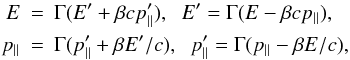 (1)where
p ∥ = pcos(θ) and
p ⊥ = psin(θ) are the
parallel and perpendicular momentum, respectively. For the relativistic case,
mc ≪ p and
mc2 ≪ E, the transformation
of the energy simplifies to E = DE′, with
D = 1/ [ Γ(1 − βcos(θ)) ] .
(1)where
p ∥ = pcos(θ) and
p ⊥ = psin(θ) are the
parallel and perpendicular momentum, respectively. For the relativistic case,
mc ≪ p and
mc2 ≪ E, the transformation
of the energy simplifies to E = DE′, with
D = 1/ [ Γ(1 − βcos(θ)) ] .
The elementary invariants under Lorentz transformations are (see, e.g., Dermer &
Menon 2010) the invariant four-volume,
dxdt = dVdt;
the invariant phase-space element,
dp/E = p2dpdΩ/E → ϵdϵdΩ,
with the final expression applying to photons and extremely relativistic particles; and the
invariant phase volume,
dν = dpdx,
where the boldface stands for three-dimensional space magnitudes. Because the number
N of particles or photons is invariant, one finds that 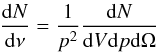 (2)is
also invariant. For photons and extremely relativistic particles, the last invariant becomes
(2)is
also invariant. For photons and extremely relativistic particles, the last invariant becomes
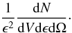 (3)Using the equality
E2 = c2p2 + m2c4
allows writing
p2dp = (pE/c2)dE.
Using the latter in Eq. (2) implies that the
expression
(3)Using the equality
E2 = c2p2 + m2c4
allows writing
p2dp = (pE/c2)dE.
Using the latter in Eq. (2) implies that the
expression 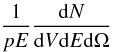 (4)is
invariant under Lorentz transformations. Again, for photons and extremely relativistic
particles, pc = E, ( = ϵ, in the notation
above for this case), and the last invariant becomes expression (3). We define the differential number density of
particles as
n(E,Ω) ≡ dN/ [ dVdEdΩ ] ,
i.e., the differential number of photons or relativistic particles with dimensionless energy
between E and E + dE that are directed
into differential solid angle interval dΩ in the direction Ω of some physical volume
dV. Because of invariant (4) and the definition of n(E,Ω), we can write
(4)is
invariant under Lorentz transformations. Again, for photons and extremely relativistic
particles, pc = E, ( = ϵ, in the notation
above for this case), and the last invariant becomes expression (3). We define the differential number density of
particles as
n(E,Ω) ≡ dN/ [ dVdEdΩ ] ,
i.e., the differential number of photons or relativistic particles with dimensionless energy
between E and E + dE that are directed
into differential solid angle interval dΩ in the direction Ω of some physical volume
dV. Because of invariant (4) and the definition of n(E,Ω), we can write
 (5)which is valid in general,
and
(5)which is valid in general,
and  (6)which is valid for photons
and extremely relativistic particles. Equation (5) just says that the expression for the distribution function
f(r,p) appearing in kinetic theory of
gases, such that the product
f(r,p)dpdV
is the number of particles lying in a given volume element dV and having
momenta in definite intervals dp, is Lorentz-invariant (see
e.g., Eq. (10.5) of Landau & Lifshitz 1987).
We note that
(6)which is valid for photons
and extremely relativistic particles. Equation (5) just says that the expression for the distribution function
f(r,p) appearing in kinetic theory of
gases, such that the product
f(r,p)dpdV
is the number of particles lying in a given volume element dV and having
momenta in definite intervals dp, is Lorentz-invariant (see
e.g., Eq. (10.5) of Landau & Lifshitz 1987).
We note that  (7)and the invariance
of f(r,p) is the one expressed by Eq. (4).
(7)and the invariance
of f(r,p) is the one expressed by Eq. (4).
2.1. The extremely relativistic case
In this case, the particle density in the jet frame transforms into the observer frame,
if it is a power law defined as  (8)by virtue of the previous
formulae ((6) and (8)), as
(8)by virtue of the previous
formulae ((6) and (8)), as 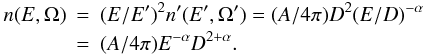 (9)
(9)
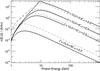 |
Fig. 1 A power-law spectrum of protons in a beam as seen by the observer for different values of viewing angles, and an example of Lorentz factor and slope (solid lines). The gray dashed lines stand for the earlier derivation results for the same parameters (see Sect. 2.4). |
2.2. The general case
Using Eqs. (1) and the one for
E2, it is possible to find that ![Mathematical equation: \begin{eqnarray} E/E' & = & E/[\Gamma (E-\beta c p \cos(\theta))] \nonumber \\ & = & \frac{1}{ \Gamma \left(1-\beta \cos(\theta) \sqrt{1-m^2 c^4/E^2} \right) }\cdot \label{ee-T} \end{eqnarray}](/articles/aa/full_html/2011/04/aa16488-11/aa16488-11-eq41.png) (10)In
addition, using the Lorentz transformation for momenta (Eq. (1) and that
(10)In
addition, using the Lorentz transformation for momenta (Eq. (1) and that  ), one has
![Mathematical equation: \begin{eqnarray} p'^2 &=& p^2 \sin^2 (\theta) + \Gamma^2 ( p \cos(\theta) - \beta E / c)^2 ) \nonumber \\ &=& p^2 \left[ \sin^2 (\theta) + \Gamma^2 ( \cos(\theta) - \beta E / \sqrt {E^2 - m^2c^4} )^2 \right]. \label{pp-T} \end{eqnarray}](/articles/aa/full_html/2011/04/aa16488-11/aa16488-11-eq43.png) (11)Using
the latter expression to get p/p′ and inserting it
into Eq. (5), together with Eqs. (8) and (10) we get,
(11)Using
the latter expression to get p/p′ and inserting it
into Eq. (5), together with Eqs. (8) and (10) we get, ![Mathematical equation: \begin{eqnarray} \label{final} n(E,\Omega) &=& \frac{ A}{4\pi} \\ &&\times \frac{ \Gamma^{-\alpha-1} E^{-\alpha} (1-\beta \cos(\theta) \sqrt{1-m^2 c^4/E^2})^{-\alpha-1} } { \left[ \sin^2 (\theta) + \Gamma^2 \left( \cos(\theta) - \frac{ \beta }{ \sqrt {1 - m^2c^4 / E^2} } \right)^2 \right]^{1/2} }\cdot \nonumber \end{eqnarray}](/articles/aa/full_html/2011/04/aa16488-11/aa16488-11-eq45.png) (12)In
the limit when mc2 ≪ E, the
last expression reduces to
(A/4π)E − αD2 + α.
To prove this we use
(12)In
the limit when mc2 ≪ E, the
last expression reduces to
(A/4π)E − αD2 + α.
To prove this we use  which can be established by
squaring both sides, and then by summing and subtracting
Γ2sin2(θ) + Γ2β2cos2(θ)
on the lefthand side, with additional use of the definition of
Γ2 = 1/ [ 1 − β2 ] . Also we do not assume a
specific jet composition, so it is a general result for any kind of particle
distributions. Figure 1 shows the resulting
expression (12) for a power-law spectrum
of protons in a beam as seen by the observer, for different values of viewing angles, and
an example of Lorentz factor and slope (solid lines). For high energies, when
E > Γmc2,
n(E,Ω) is a power-law distribution, as the original
primed one, albeit it presents a different behavior for lower values of
E.
which can be established by
squaring both sides, and then by summing and subtracting
Γ2sin2(θ) + Γ2β2cos2(θ)
on the lefthand side, with additional use of the definition of
Γ2 = 1/ [ 1 − β2 ] . Also we do not assume a
specific jet composition, so it is a general result for any kind of particle
distributions. Figure 1 shows the resulting
expression (12) for a power-law spectrum
of protons in a beam as seen by the observer, for different values of viewing angles, and
an example of Lorentz factor and slope (solid lines). For high energies, when
E > Γmc2,
n(E,Ω) is a power-law distribution, as the original
primed one, albeit it presents a different behavior for lower values of
E.
2.3. A power law with an exponential cutoff
We also briefly consider the case in which the intrinsic particle distribution in the
beam is a power law with an exponential cutoff. This would be a natural consequence of
particles being subject to losses on the same site as where they are accelerated. As such,
the cutoff appears in the primed referenced frame, where  (13)Here,
Ecut should be fixed in the beam frame, where acceleration
and losses are supposed to occur, but once fixed it is not subject to Lorentz
transformations. However, the energy variable in the exponential function is. The result
is
(13)Here,
Ecut should be fixed in the beam frame, where acceleration
and losses are supposed to occur, but once fixed it is not subject to Lorentz
transformations. However, the energy variable in the exponential function is. The result
is ![Mathematical equation: \begin{eqnarray} \label{final-cut} n(E,\Omega) &=& \frac{ A}{4\pi} \\ && \times \frac{ \Gamma^{-\alpha-1} E^{-\alpha} (1-\beta \cos(\theta) \sqrt{1-m^2 c^4/E^2})^{-\alpha-1} } { \left[ \sin^2 (\theta) + \Gamma^2 \left( \cos(\theta) - \frac{ \beta }{ \sqrt {1 - m^2c^4 / E^2} } \right)^2 \right]^{1/2} } \nonumber \\ && \times \exp \left( -\frac{\Gamma E } {E_{\rm cut}} (1-\beta \cos(\theta) \sqrt{1- m^2c^4/E^2} \right). \nonumber \end{eqnarray}](/articles/aa/full_html/2011/04/aa16488-11/aa16488-11-eq53.png) (14)When
mc2 ≪ E, the exponential
cutoff exp( − E′/Ecut) is transformed into
exp( − E/DEcut), with
D the bulk Doppler factor.
(14)When
mc2 ≪ E, the exponential
cutoff exp( − E′/Ecut) is transformed into
exp( − E/DEcut), with
D the bulk Doppler factor.
2.4. Comparison with Purmohammad & Samimi (2001)
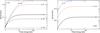 |
Fig. 2 Comparison of the derived expression for the spectrum of protons in beams, following Eq. (22). Left: a function of the viewing angle (θ) for Γ = 10. Right: a function of the bulk Lorentz factor (Γ), for θ = 20°. |
Purmohammad & Samimi (2001, hereafter PS01)
state that the isotropic particle distribution transformed from the jet into the observer
frame results in (in this section and to avoid confusion we label their expressions with
⋆ ): ![Mathematical equation: \begin{eqnarray} \label{them-general} n_\star(E,\Omega) &= &\frac{A}{4\pi} \Gamma^{-\alpha+1} E^{-\alpha} \\ && \times \frac {(1-\beta \cos(\theta) \sqrt{1-m^2 c^4/E^2} )^{-\alpha} } { \left[ \sin^2 \theta +\Gamma^2 \left(\cos(\theta)- \frac{\beta }{ \sqrt{1-m^2 c^4/E^2}}\right)^2 \right]^{1/2} }\cdot \nonumber \end{eqnarray}](/articles/aa/full_html/2011/04/aa16488-11/aa16488-11-eq62.png) (15)Purmohammad
&Samimi’s (2001) paper does not provide a
derivation of their Eq. (3), quoted above as (15), but earlier private communication with one of us was sufficient to
reconstruct it, as follows. They start by assuming conservation of particles in the form
(15)Purmohammad
&Samimi’s (2001) paper does not provide a
derivation of their Eq. (3), quoted above as (15), but earlier private communication with one of us was sufficient to
reconstruct it, as follows. They start by assuming conservation of particles in the form
 (16)thus one has
 (17)From the
Lorentz-invariance of the phase-space element
dp/E, the invariance of
pdΩdE can also be proved. Then, one can write
(17)From the
Lorentz-invariance of the phase-space element
dp/E, the invariance of
pdΩdE can also be proved. Then, one can write
 (18)Using the
expressions derived above for p/p′ and the equality
dV′ = ΓdV into (17), one gets
(18)Using the
expressions derived above for p/p′ and the equality
dV′ = ΓdV into (17), one gets 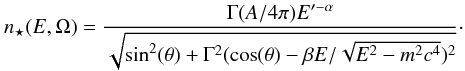 (19)From here, after
replacing in the numerator
(19)From here, after
replacing in the numerator  ,
expression (15) follows immediately.
,
expression (15) follows immediately.
Formally, one can say that there is a problem hidden in Eq. (16), from which the rest of the derivation
follows. The invariant phase volume is not dVdΩdE but
rather p2dVdΩdp. To avoid
inconsistencies, invariants (from which to derive transformation laws) should be written
as operations over individually invariant factors, e.g., dN over
dν, rather than from identities (which is what one obtains by replacing
the definition of n and n′ in Eq. (16)). However, the latter can also yield the
correct result, too, if care is exercised. In practice, then, the problem with the prior
derivation is in the use of the equality dV′ = ΓdV. This
equation implies that dV′ is the proper volume
dV0, which is clearly incorrect, given that the momentum,
p′, of the particles
in that volume is not zero. Only for the proper volume is the referred equality true (see,
e.g., Eq. (4.6) of Landau & Lifshitz 1987).
To clarify this issue, let us introduce, in addition of the two reference systems
(observer and beam), another frame K0 in which the particles
with the given momentum are at rest. The proper volume dV0 of
the element occupied by the particles is defined relative to this system. The velocities
of the primed and unprimed systems relative to the system K0
coincide by definition with the velocities v and v′,
which these particles have in the systems of the observer and the beam, respectively.
Thus, we can write  (20)from
which one can write
(20)from
which one can write  (21)If we use
Eqs. (18) and (21) in Eq. (16), the last transforms back into the expression of the invariant
quantity
1/(pE) × dN/(dVdEdΩ)
and Eq. (5) follows.
(21)If we use
Eqs. (18) and (21) in Eq. (16), the last transforms back into the expression of the invariant
quantity
1/(pE) × dN/(dVdEdΩ)
and Eq. (5) follows.
The difference between expression (15)
and our Eq. (12) is important. Dividing
one by another, we obtain  (22)which is a non-trivially
dependent function of Γ, E, and θ. However, it is not a
function of α. In the extremely relativistic case
mc2 ≪ E, one notices a
factor D/Γ of difference. Put otherwise, in the stated asymptotic
regime, the ratio expressed by Eq. (22)
reduces to
(22)which is a non-trivially
dependent function of Γ, E, and θ. However, it is not a
function of α. In the extremely relativistic case
mc2 ≪ E, one notices a
factor D/Γ of difference. Put otherwise, in the stated asymptotic
regime, the ratio expressed by Eq. (22)
reduces to  ,
which is only a function of Γ and θ. One can see that, in the case of
θ = 0°,
n(E,Ω)/n ⋆ (E,Ω) → 2
for growing Γ. For other values of θ, this 2D function quickly falls off.
We plot the comparison between our derivation and the one by PS01 in Fig. 2, both as a function of viewing angle θ
(for fixed Γ = 10) and bulk Lorentz factor Γ (for θ = 20°). We see that
the differences range from a factor of ~2 in the case of directly-pointing
beams of blazars and microblazars (of very low θ, in our example, 0.6°),
to one order of magnitude at least for the more common cases of moderate inclinations
(e.g., for 20°; with the difference being significantly larger for larger inclinations).
As soon as θ is larger than ~5°, the proton spectrum in the
beam increasingly undershoots PS01’s calculation. This leads to an analogous correction of
previously calculated γ-ray and neutrino emission (typically by more than
one order of magnitude) in all cases in which expression (15) was used. In the low energy decline, PS01’s calculation always
overestimates (by about two orders of magnitude) the correct yield of the proton spectrum
(see Fig. 1 at proton energies between 1 and 10 GeV).
,
which is only a function of Γ and θ. One can see that, in the case of
θ = 0°,
n(E,Ω)/n ⋆ (E,Ω) → 2
for growing Γ. For other values of θ, this 2D function quickly falls off.
We plot the comparison between our derivation and the one by PS01 in Fig. 2, both as a function of viewing angle θ
(for fixed Γ = 10) and bulk Lorentz factor Γ (for θ = 20°). We see that
the differences range from a factor of ~2 in the case of directly-pointing
beams of blazars and microblazars (of very low θ, in our example, 0.6°),
to one order of magnitude at least for the more common cases of moderate inclinations
(e.g., for 20°; with the difference being significantly larger for larger inclinations).
As soon as θ is larger than ~5°, the proton spectrum in the
beam increasingly undershoots PS01’s calculation. This leads to an analogous correction of
previously calculated γ-ray and neutrino emission (typically by more than
one order of magnitude) in all cases in which expression (15) was used. In the low energy decline, PS01’s calculation always
overestimates (by about two orders of magnitude) the correct yield of the proton spectrum
(see Fig. 1 at proton energies between 1 and 10 GeV).
3. Discussion
The proton-beam model presented by PS01 gives an expression for a power-law proton spectrum in a beam, as seen by the observer. We have demonstrated that this expression is incorrect, since it does not comply with relativistic invariants. We derived the correct transformation from the jet frame particle density to the observer’s, which strictly obeys these Lorentz invariance constraints. By comparing our result with PS01, we noticed that differences depend strongly on the viewing angle. For many cases, PS01 calculation entails a significant overprediction (order of magnitude) of the proton spectra for E > Γmc2, whereas it always significantly overpredicts (two orders of magnitude) the proton spectrum at lower energies, for all viewing angles. The γ-ray luminosity is related to the particle density through the corresponding emissivity of the processes by which the particles interact. For instance, the charged and neutral pion decay channels are the most effective yield of photons and neutrinos in many situations, and its emissivity is directly proportional to the particle density n(E,Ω). Many publications that rely on the calculation by PS01 for estimating γ-ray and neutrino emission yields in hadronic beam scenarios are thus affected in this way.
One particular example can be seen in the hadronic MQ case (Romero et al. 2003)1 and in their applications (e.g., Romero et al. 2005; Orellana et al. 2007; Reynoso et al. 2008). These are all affected by our results. MQs can have Γ ~ 2, but θ-values above 10° are typical. MQs can precess, as for SS433, where θ can even change up to 20° around an already large mean viewing angle.
Only a small part of the γ-ray AGNs are not blazars. The majority among those associated with radio sources possess relatively large core dominance (Abdo et al. 2010), indicating that their viewing angle is probably not large. Assuming θ < 20°, if Γ < 10, PS01 deviation is no more than a factor of ~6 (at E > mc2). For the average blazar with Γ = 10 and θ < 10° the difference is a factor of ~2. However, it has been argued that during the extreme TeV flaring events of some blazars (e.g. Mkn 501, PKS 2155-304), Lorentz factors greater than Γ ~ 50 are required (e.g. Begelman et al. 2008). If the viewing angle remains at θ ~ 1/Γquiet ~ 1/10 ~ 5.7° during such events, PS01 formulation error can grow to more than an order of magnitude. Furthermore, a few radio galaxies with large viewing angles are also detected at γ-ray energies: M87 with viewing angle θ < ~ 40°, and Cen A where estimates for the viewing angle range from 15° to 80°. These radio galaxies have been already modeled with the PS01 derivation (e.g., Reynoso et al. 2010). Here, the difference between the PS01 formula and ours can reach a factor 20 for Γ not larger than 5.
Finally, we note that models designed to predict future detections of large-viewing angle sources with higher sensitivity instruments than currently available will strongly overpredict the number of sources if the PS01 formula is used. Similarly, a model for an AGN that overestimates the γ-ray flux could make wrong associations of unidentified γ-ray sources. Given that γ-ray fluxes will be diminished in many cases, and that the time of observations in Cherenkov facilities grows with the square of the flux-reduction factor, the likelihood of observing hadronic beams is undermined.
Note that the Eq. (2) in the latter paper has a missing square in the denominator factor
 . This error has been adopted in
several of the papers quoting Romero et al. (2003).
. This error has been adopted in
several of the papers quoting Romero et al. (2003).
Acknowledgments
D.F.T. acknowledges support from grants AYA2009-07391, SGR2009-811, and TW2010005. A.R. acknowledges support by the Marie Curie IRG grant 248037 within the FP7 Program. We acknowledge O. Reimer for discussions.
References
- Abdo, A., Ackermann, M., Ajello, M., et al. 2010, ApJ, 720, 912 [NASA ADS] [CrossRef] [Google Scholar]
- Begelman, M., Fabian, A. C., & Rees, M. J. 2008, MNRAS, 384, L19 [NASA ADS] [CrossRef] [Google Scholar]
- Dermer, C., & Menon, G. 2010, High-Energy Radiation from Black Holes (Oxford University Press) [Google Scholar]
- Landau, L., & Lifshitz, E. M. 1987, Theory of Fields, fourth revised English edn. (Buttenworth-Heinemann) [Google Scholar]
- Purmohammad, D., & Samimi, J. 2001, A&A, 371, 61 (PS01) [NASA ADS] [CrossRef] [EDP Sciences] [Google Scholar]
- Orellana, M., Bordas, P., Bosch-Ramon, V., Romero, G. E., & Paredes, J. M. 2007, A&A, 476, 9 [NASA ADS] [CrossRef] [EDP Sciences] [Google Scholar]
- Romero, G. E, Torres, D. F., Kaufman-Bernadó, M. M., & Mirabel, I. F. 2003, A&A, 410, L1 [NASA ADS] [CrossRef] [EDP Sciences] [Google Scholar]
- Romero, G. E, Christiansen, H. R., & Orellana, M. 2005, APJ, 632, 1093 [Google Scholar]
- Reynoso, M. M., Romero, G. E., & Christiansen, H. R. 2008, MNRAS, 387, 1745 [NASA ADS] [CrossRef] [Google Scholar]
- Reynoso, M. M., Medina, M. C., & Romero, G. E. 2010, A&A, submitted [arXiv:1005.3025v1] [Google Scholar]
All Figures
|
Fig. 1 A power-law spectrum of protons in a beam as seen by the observer for different values of viewing angles, and an example of Lorentz factor and slope (solid lines). The gray dashed lines stand for the earlier derivation results for the same parameters (see Sect. 2.4). |
| In the text | |
|
Fig. 2 Comparison of the derived expression for the spectrum of protons in beams, following Eq. (22). Left: a function of the viewing angle (θ) for Γ = 10. Right: a function of the bulk Lorentz factor (Γ), for θ = 20°. |
| In the text | |
Current usage metrics show cumulative count of Article Views (full-text article views including HTML views, PDF and ePub downloads, according to the available data) and Abstracts Views on Vision4Press platform.
Data correspond to usage on the plateform after 2015. The current usage metrics is available 48-96 hours after online publication and is updated daily on week days.
Initial download of the metrics may take a while.