| Issue |
A&A
Volume 528, April 2011
|
|
|---|---|---|
| Article Number | L3 | |
| Number of page(s) | 4 | |
| Section | Letters | |
| DOI | https://doi.org/10.1051/0004-6361/201016175 | |
| Published online | 17 February 2011 | |
Letters to the Editor
First evidence of a gravitational lensing-induced echo in gamma rays with Fermi LAT
1
DSM/IRFU, CEA/Saclay, 91191
Gif-sur-Yvette,
France
e-mail: This email address is being protected from spambots. You need JavaScript enabled to view it.
2
Nicolaus Copernicus Astronomical Center,
Warszawa,
Poland
e-mail: This email address is being protected from spambots. You need JavaScript enabled to view it.
Received:
19
November
2010
Accepted:
24
January
2011
Abstract
Aims. This article shows the first evidence ever of gravitational lensing phenomena in high energy gamma-rays. This evidence comes from the observation of an echo in the light curve of the distant blazar PKS 1830-211 induced by a gravitational lens system.
Methods. Traditional methods for estimating time delays in gravitational lensing systems rely on the cross-correlation of the light curves from individual images. We used the 300 MeV–30 GeV photons detected by the Fermi-LAT instrument. It cannot separate the images of known lenses, so the observed light curve is the superposition of individual image light curves. The Fermi-LAT instrument has the advantage of providing long, evenly spaced, time series with very low photon noise. This allows us to use Fourier transform methods directly.
Results. A time delay between the two compact images of PKS 1830-211 has been searched for by both the autocorrelation method and the “double power spectrum” method. The double power spectrum shows a 4.2σ proof of a time delay of 27.1 ± 0.6 days, consistent with others’ results.
Key words: gravitational lensing: strong / quasars: individual: PKS 1830-211 / methods: data analysis
© ESO, 2011
1. Introduction
Precise estimation of the time delay between components of lensed active galactic nuclei (AGN) is crucial for modeling the lensing objects. In turn, more accurate lens models give better constraints on the Hubble constant. More than 200 strong lens systems have been discovered, most of them in recent years by dedicated surveys such as the Cosmic Lens All-Sky Survey (Myers et al. 2003; Browne et al. 2003) and the Sloan Lens ACS Survey (Bolton et al. 2004). The launch of the Fermi satellite (Atwood et al. 2009) in 2008 offered the opportunity to investigate gravitational lensing phenomena with high-energy gamma rays. The observation strategy of Fermi-LAT, which surveys the whole sky in 190 min, allows a regular sampling of quasar light curves with a period of a few hours. This paper deals with the observation and estimation of time delays in strong lensing systems and not with the detection and use of microlensing phenomena such as in Torres et al. (2003).
The multiple images of a gravitational lensed AGN cannot be directly observed with high energy gamma-ray instruments such as Fermi-LAT, Swift, or ground-based Cerenkov telescopes, owing to their limited angular resolutions. The angular resolution of these instruments is at best a few arcminutes (in the case of HESS), when the typical separation of the images for quasar lensed by galaxies is a few arcseconds. This paper is concerned with estimating the time delay in strong lenses when only spatially unresolved data are available. Spectral analysis techniques and echo detection methods are investigated. A similar approach to detecting GRB lensing has been proposed by Wambsganss (1993).
Our methods of time-delay estimation have been tested on simulated light curves and on the Fermi LAT observations of the very bright radio quasar PKS 1830-211, for which the time delay was previously estimated by Lovell et al. (1998) using radio observations. The paper is organized as follows. We first give a very brief summary of properties of PKS 1830-211 and of Fermi LAT data towards this AGN. We next introduce the methods for estimating the time delay. The last section is devoted to measuring the time delay between the two compact components of PKS 1830-211.
2. The PKS 1830-211 gravitational lens system
The AGN PKS 1830-211 is a variable, bright radio source and an X-ray blazar. Its redshift has been measured to be z = 2.507 (Lidman et al. 1999). The blazar was detected in the γ-ray wavelengths with EGRET. The EGRET source was associated with the radio source by Mattox et al. (1997). The classification of PKS 1830-211 as a gravitationally lensed quasi-stellar object was first proposed by Pramesh Rao & Subrahmanyan (1988). The lensing galaxy is a face-on spiral galaxy, which was identified by Winn et al. (2002) and Courbin et al. (2002), and it is located at redshift z = 0.89 (Wiklind & Combes 1996).
PKS 1830-211 is observed in radio as an elliptical ring-like structure connecting two bright sources roughly one arcsecond distant (Jauncey et al. 1991). The compact components were separately observed by the Australia Telescope Compact Array at 8.6 GHz for 18 months. These observations and the subsequent analysis by Lovell et al. (1998) give a magnification ratio between the 2 images of 1.52 ± 0.05 and a time delay of  days. A separate measurement of a time delay of
  days has been made by Wiklind & Combes (2001) using molecular absorption lines.
 |
Fig. 1 Fermi LAT light curve of PKS 1830-211, with a two-day binning. The energy range is 300 MeV to 300 GeV. |
3. Fermi LAT data on PKS 1830-211
PKS 1830-211 has been detected by the Fermi LAT instrument with a detection significance above 41 Fermi Test Statistic (TS), equivalent to a 6σ effect (Abdo et al. 2010). The long-term light curve is presented in Fig. 1 with a two-day binning. The data analysis from this paper uses a two-day binning, which provides a sufficient photon statistic per bin with a time span per bin that is much shorter than 28 days. The data analysis was cross-checked by binning the light curve into one day and 23-h bins, with similar results. The data were taken between August 4, 2008 and October 13, 2010 and processed by the publicly available Fermi Science Tools version 9. The v9r15p2 software version and the P6_V3_DIFFUSE instrument response functions were used. The light curve was produced by aperture photometry selecting photons from a region with radius 0.5 deg around the nominal position of PKS 1830-211 and energies between 300 MeV and 300 GeV.
4. Data processing and method
4.1. Idea
If a distant source (in our case an AGN) is gravitationally lensed, the light reaches the observer by at least two different paths. We assume here that there are only two light paths. In reality, the light curves of the two images are not totally identical since (in addition to differences due to photon noise) the source can be microlensed in one of the two paths. Neglecting for the moment the background light and the differences due to microlensing, the observed flux can be decomposed into two components. One of the components is the intrinsic AGN light curve, given by f(t), with Fourier transform  The other component has a similar time evolution to the first one, but is shifted in time with a delay a. In addition, the brightness of the second component differs by a factor b from that of the first component, so that it can be written as bf(t + a), and its transform to the Fourier space gives
  .
.
The sum of two component gives g(t) = f(t) + bf(t + a), which transforms into  in Fourier space. The power spectrum Pν of the source is obtained by computing the square modulus of
  :
:  (1)The measured Pν is the product of the “true” power spectrum of the source times a periodic component with a period (in the frequency domain) equal to the inverse of the relative time delay a. The microlensing of one of the components, if taken into account, gives a modulation of the amplitude of the oscillatory pattern at low frequencies. Since the typical duration of a caustic crossing microlensing event is a few months, only frequencies under 3 × 10⁻⁷ Hz will be affected.
The usual way to measure the time delay a is to calculate the autocorrelation function of f(t). This method was investigated by Geiger & Schneider (1996). Computation of the autocorrelation of a light curve with uneven sampled data is described in Edelson & Krolik (1988). The Fermi light curve of PKS 1830-211 has very few gaps, and only one notable four-day gap. The missing data have been linearly interpolated. However, simulations with an artificial gap have shown that the results of the present paper are not affected by this gap. The autocorrelation function can be written as the sum of three terms. One of these terms models the “intrinsic” autocorrelation of the AGN, decreasing with a time constant λ. If λ is larger than a, the autocorrelation method fails, because the time delay peak merges with the intrinsic component of the AGN. Another potential problem with the autocorrelation method is the sensitivity to spurious periodicities such as the one coming from the motion and rotation of the Fermi satellite.
The periodic modulation of Pν suggests the use of another method, based on the computation of the power spectrum of Pν, noted Da. This method is similar in spirit to the cepstrum analysis (Bogert et al. 1963) used in seismology and speech processing. If  were a constant function of ν, Da would have a peak at the time delay a. In the general case, Da is obtained by the convolution of a Dirac function, coming from the cosine modulation, by the Fourier transform of the function:
  (2)where W(0, νmax) is the window in frequency of Pν and νmax is maximum available frequency. The Fourier transform h(a) of
  defines the width of the time delay peak in the double power spectrum Da. For instance if
  and λW ≫ 1, then the time delay peak in Da has a Lorentzian shape with a FWHM of λ/π. For a typical value of λ = 10 days, one has a FWHM of 3 days.
In the next section we describe the calculation of Pν and Da and illustrate the procedure with Monte Carlo simulations.
4.2. Power spectrum
To avoid problems arising from the finite length of measurements, sampling and aliasing, we use the procedure for data reduction described by Brault & White (1971) and Press et al. (2007).
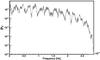 |
Fig. 2 Simulated power spectrum of a lensed AGN with a time delay of 28 days between images. The power Pν is in arbitrary units. |
The artificial light curve was produced by summing three simulated components. The light curve of PKS 1830-211 shown in Fig. 1 does not exhibit any easily recognized features, but it does have a rather random-like aspect. The first component was thus simulated as white noise with a Poisson distribution. It would be more realistic to use red noise instead of white noise, but the latter is sufficient for most of our purposes, such as computing Da. The second component is obtained from the first by shifting the light curve with a 28-day time lag. The effect of differential magnification of the images has also been included. The background photon noise was taken into account by adding a third component with a Poisson distribution.
The mean number of counts per two-day bin for PKS 1830-211 is 5.42. This value was used to generate artificial light curves. The first and second components account for 80% of the simulated count rate and the rest is contributed by the Poisson noise.
4.3. Time delay determination
The methods of time delay determination use the power spectrum Pν as described in the previous section. The simulated Pν presented in Fig. 2 shows a very clear periodic pattern. From Eq. (1) we know that the period of the observed oscillations equals the inverse of the time delay between the images.
Our preferred approach was to calculate the double power spectrum Da. As in Sect. 4.2, the power spectrum Pν has to be prepared before undergoing a Fourier transform to the “time delay” domain. The low-frequency part (ν < 1/55 day-1) of Pν is cut off. This cut arises because of the strong power observed at low frequencies in the power spectrum of PKS 1830-211. The high-frequency part of the spectrum Pν is also removed because the power at high frequency is low. (It goes to 0 at the Nyquist frequency.) Calculation of Da proceeds like in Sect. 4.2, except that the Pν data are bent to zero by multiplication with a cosine bell. The Da distribution is estimated from five segments of the light curve. In every bin of the Da distribution, the estimated double power spectrum is given by the average over the five segments. The errors bars on Da are estimated from the dispersion of bin values divided by two (since there are five segments). Due to the random nature of the sampling process, some of the error bars obtained are much smaller than the typical dispersion in the Da points. To take this into account, a small systematic error bar was added quadratically to all points. The result (with statistical error bars only) is presented in Fig. 3.
 |
Fig. 3 Double power spectrum Da for the simulated lensed AGN of Fig. 2. Da is plotted in arbitrary units. The solid line is a fit to a linear plus Gaussian profile. |
 |
Fig. 4 Autocorrelation function of the simulated lensed AGN of Fig. 2. The solid line is a fit to a linear plus Gaussian profile. |
As mentioned in Sect. 4.1, the usual approach for time delay estimation is to compute the autocorrelation of the light curve. The auto-covariance is obtained by taking the real part of the inverse Fourier transform of Pν. The auto-covariance is normalized (divided by the value at zero time lag) to get the autocorrelation. The autocorrelation function of an artificial light curve simulated as in Sect. 4.2 is presented in Fig. 4.
A peak with a significance of roughly 16σ is present at 27.85 ± 0.14 days, however, the significance of this peak is overestimated since light curves are simulated with white noise instead of red noise. The autocorrelation function of a light curve driven by red noise is given by e − a/λ. For our simulated light curves, λ = 0, so that the peak is a hardly affected by the background of the AGN.
For the simulated light curves, both approaches of time delay determination give reasonable and compatible results.
 |
Fig. 5 Measured power spectrum of PKS 1830-211, plotted in arbitrary units. |
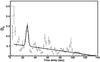 |
Fig. 6 Double power spectrum of PKS 1830-211 plotted in arbitrary units. The solid line is a fit to a linear plus Gaussian profile. |
5. Results and discussion
The results for real data were obtained with the same procedure as for the simulated light curves. Figure 5 shows the power spectrum Pν calculated from the light curve of PKS 1830-211. An oscillatory pattern is clearly visible in the power spectrum. It is similar to the pattern expected from the simulations shown in Fig. 2. The autocorrelation function and the Da distribution calculated for real data are shown in Figs. 7 and 6. A peak around 27 days is seen in both distributions. Several other peaks are present on the autocorrelation function as already noted by Geiger & Schneider (1996, see their Fig. 1). The peak around five days in the Da distribution is likely to be an artefact of the time variation of the exposure of the LAT instrument on PKS 1830-211. Using the method described in Sect. 4.3, the significance of the peak around 27 days is found to be 1.1σ in the autocorrelation function and 4.2σ in the double power spectrum Da. Fitting the position of the peak gives the time delay of a = 27.1 ± 0.6 days for the Da distribution. The fit of the autocorrelation function to a Gaussian peak over an exponential background gives a = 27.1 ± 0.45 days. In both cases, the quoted error is derived from the fit.
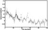 |
Fig. 7 Measured autocorrelation function of PKS 1830-211. The solid line is a fit to an exponential plus Gaussian profile. |
References
- Abdo, A. A., Ackermann, M., Ajello, M., et al. 2010, VizieR Online Data Catalog, 218, 80405 [NASA ADS] [Google Scholar]
- Atwood, W. B., Abdo, A. A., Ackermann, M., et al. 2009, ApJ, 697, 1071 [NASA ADS] [CrossRef] [Google Scholar]
- Bogert, B. P., Healy, M. J. R., & Tukey, J. W. 1963, in Proceedings on the Symposium on Time Series Analysis, ed. M.Rosenblat (NY: Wiley), 209 [Google Scholar]
- Bolton, A. S., Burles, S., Schlegel, D. J., Eisenstein, D. J., & Brinkmann, J. 2004, AJ, 127, 1860 [NASA ADS] [CrossRef] [Google Scholar]
- Brault, J. W., & White, O. R. 1971, A&A, 13, 169 [NASA ADS] [Google Scholar]
- Browne, I. W., Wilkinson, P. N., Jackson, N. J., et al. 2003, MNRAS, 341, 13 [NASA ADS] [CrossRef] [Google Scholar]
- Courbin, F., Meylan, G., Kneib, J., & Lidman, C. 2002, ApJ, 575, 95 [Google Scholar]
- Edelson, R. A., & Krolik, J. H. 1988, ApJ, 333, 646 [NASA ADS] [CrossRef] [Google Scholar]
- Geiger, B., & Schneider, P. 1996, MNRAS, 282, 530 [NASA ADS] [Google Scholar]
- Jauncey, D. L., Reynolds, J. E., Tzioumis, A. K., et al. 1991, Nature, 352, 132 [NASA ADS] [CrossRef] [Google Scholar]
- Lidman, C., Courbin, F., Meylan, G., et al. 1999, ApJ, 514, L57 [Google Scholar]
- Lovell, J. E. J., Jauncey, D. L., Reynolds, J. E., et al. 1998, ApJ, 508, L51 [Google Scholar]
- Mattox, J. R., Schachter, J., Molnar, L., Hartman, R. C., & Patnaik, A. R. 1997, ApJ, 481, 95 [NASA ADS] [CrossRef] [Google Scholar]
- Myers, S. T., Jackson, N. J., Browne, I. W. A., et al. 2003, MNRAS, 341, 1 [NASA ADS] [CrossRef] [Google Scholar]
- Pramesh Rao, A., & Subrahmanyan, R. 1988, MNRAS, 231, 229 [NASA ADS] [Google Scholar]
- Press, W. H., Teukolsky, S. A., Vetterling, W. T., & Flannery, B. P. 2007, Numerical Recipes, The Art of Scientific Computing, 3rd edn. (Cambridge University Press) [Google Scholar]
- Torres, D. F., Romero, G. E., Eiroa, E. F., Wambsganss, J., & Pessah, M. E. 2003, MNRAS, 339, 335 [NASA ADS] [CrossRef] [Google Scholar]
- Wambsganss, J. 1993, ApJ, 406, 29 [NASA ADS] [CrossRef] [Google Scholar]
- Wiklind, T., & Combes, F. 1996, in Cold Gas at High Redshift, ed. M. N. Bremer, & N. Malcolm, Astrophysics and Space Science Library, 206, 227 [Google Scholar]
- Wiklind, T., & Combes, F. 2001, in Gravitational Lensing: Recent Progress and Future Go, ed. T. G. Brainerd, & C. S. Kochanek, ASP Conf. Ser., 237, 155 [Google Scholar]
- Winn, J. N., Kochanek, C. S., McLeod, B. A., et al. 2002, ApJ, 575, 103 [NASA ADS] [CrossRef] [Google Scholar]
All Figures
|
Fig. 1 Fermi LAT light curve of PKS 1830-211, with a two-day binning. The energy range is 300 MeV to 300 GeV. |
| In the text | |
|
Fig. 2 Simulated power spectrum of a lensed AGN with a time delay of 28 days between images. The power Pν is in arbitrary units. |
| In the text | |
|
Fig. 3 Double power spectrum Da for the simulated lensed AGN of Fig. 2. Da is plotted in arbitrary units. The solid line is a fit to a linear plus Gaussian profile. |
| In the text | |
|
Fig. 4 Autocorrelation function of the simulated lensed AGN of Fig. 2. The solid line is a fit to a linear plus Gaussian profile. |
| In the text | |
|
Fig. 5 Measured power spectrum of PKS 1830-211, plotted in arbitrary units. |
| In the text | |
|
Fig. 6 Double power spectrum of PKS 1830-211 plotted in arbitrary units. The solid line is a fit to a linear plus Gaussian profile. |
| In the text | |
|
Fig. 7 Measured autocorrelation function of PKS 1830-211. The solid line is a fit to an exponential plus Gaussian profile. |
| In the text | |
Current usage metrics show cumulative count of Article Views (full-text article views including HTML views, PDF and ePub downloads, according to the available data) and Abstracts Views on Vision4Press platform.
Data correspond to usage on the plateform after 2015. The current usage metrics is available 48-96 hours after online publication and is updated daily on week days.
Initial download of the metrics may take a while.