| Issue |
A&A
Volume 528, April 2011
|
|
|---|---|---|
| Article Number | A68 | |
| Number of page(s) | 8 | |
| Section | Astronomical instrumentation | |
| DOI | https://doi.org/10.1051/0004-6361/201015903 | |
| Published online | 03 March 2011 | |
Monitoring the solar UV irradiance spectrum from the observation of a few passbands
1 LPC2E, UMR 6115, CNRS and University
of Orléans, 3A avenue de la Recherche
Scientifique, 45071 Orléans Cedex
2, France
e-mail: This email address is being protected from spambots. You need JavaScript enabled to view it.
2 LPG, UMR 5109, CNRS and University of Joseph Fourier,
Bâtiment D de Physique, BP 53, 38041 Saint-Martin d’Hères Cedex 9, France
3 LATMOS, UMR 8190, CNRS,
11 boulevard
D’Alembert, 78280
Guyancourt,
France
4 Observatoire Royal de Belgique,
Avenue Circulaire
3, 1800
Brussels,
Belgium
5 Laboratory for Atmospheric and Space
Physics, University of Colorado, 1234 Innovation Dr., Boulder, CO
80303,
USA
Received: 10 October 2010
Accepted: 10 January 2011
Abstract
Context. The solar irradiance in the UV is a key ingredient in space weather applications; however, because of the lack of continuous and long-term observations, various indices are still used today as surrogates for the solar spectral irradiance.
Aims. As an alternative to current spectrometers we use a few radiometers with properly chosen passbands and reconstruct the solar spectral irradiance from their outputs. The feasibility of such a reconstruction is justified by the high redundancy in the spectral variability.
Methods. Using a multivariate statistical approach, we first compared six years of daily-averaged UV spectra and a selection of passbands (from existing radiometers) and solar indices. This leads to a strategy for defining those passbands that are most appropriate for reconstructing the spectrum.
Results. With four passdbands chosen from already existing instruments, we reconstruct the UV spectrum with a relative error of about 20%. Better performance is achieved with a combination of passbands than with a combination of indices.
Key words: Sun: UV radiation / instrumentation: photometers / methods: statistical / methods: data analysis
© ESO, 2011
1. Introduction
The solar irradiance in the ultraviolet (UV) is a key parameter for solar terrestrial physics (Lilensten et al. 2008). Now, casting the solar UV variability is also extremely important for climate modelling (see Gray et al. 2010, for a review). In solar physics, the most energetic part of the solar UV spectrum is conventionally divided into middle UV (MUV, 200–300 nm), far UV (FUV, 122–200 nm), extreme UV (EUV, 10–121 nm), and soft X-rays (XUV, 0.1–10 nm) (Tobiska & Nusinov 2006). Different classifications are used in other domains, such as in medicine. The solar spectral variability in the UV is complex and highly dynamic, and it directly affects the thermosphere/ionosphere system. Various space weather applications, such as orbit determination, satellite communications, and positioning require a continuous and radiometrically calibrated monitoring of the solar spectral irradiance in the UV. It is also necessary to understand how the solar UV variability may affect climate directly or indirectly. Many chemical cycles are indeed affected by the solar spectral irradiance in the UV (Egorova et al. 2004).
The long-term monitoring of the UV, however, is a major challenge. Measurements must be carried out in space, where current instruments suffer from ageing, degradation, and signal contamination. Until 2003, when the SORCE satellite started operating, there was no continuous monitoring of the complete UV spectrum. This lack of data has been particularly severe in the EUV range, and was termed the “EUV hole” (Schmidtke et al. 2002), which ended with the launch of the TIMED satellite in February 2002 (Woods et al. 2005).
The solar atmosphere is not in thermodynamic equilibrium and so the formation of the solar UV spectrum cannot be described by a Planck spectrum. For that reason, several physical mechanisms need to be considered. In the MUV range, several important Fraunhofer absorption lines (e.g. Mg II at 280 nm) are noticeable, which come from elements in the chromosphere and the photosphere. The MUV range, however, is dominated not by separate absorption lines but by an immense number of unresolved spectral lines that form the UV line haze (e.g. Busá et al. 2001). At the considered temperature in the upper solar atmosphere, many charged ions are involved. Intense emission lines coming from the de-excitation of these ionised atoms are a prevalent process of emission: coronal lines predominate at shorter EUV wavelengths, while those of the transition region and the chromosphere are found at longer EUV wavelengths and in the FUV range. The EUV range is, moreover, dominated by the Lyman series for H (Lyα at 121.6 nm) and by He II (Lyα at 30.4 nm), both of which are emitted in the transition region. These lines, however, are coupled with higher layers, so they cannot be assigned to a specific altitude (Vourlidas et al. 2001). Finally, the continuum of the UV spectrum is driven by free-bound and free-free processes arising in the upper photosphere. For wavelengths above 160 nm, however, the continuum mainly mainly originates in the chromosphere.
Because of this diversity of processes, the spectral variability has many degrees of freedom, and there is a priori no reason for different spectral lines to evolve similarly. One may then expect the integration of the solar spectrum over finite spectral bands to irreversibly destroy the information that is needed to reconstruct some of the spectral lines contained in these bands. As we shall see later, this is not necessarily the case, since the spectral variability is remarkably coherent.
The Sun varies on all times scales and its variability is strongly wavelength-dependent (Lean 1987). The variability on a 27-day solar rotation scale, for example, is mostly related to the appearance and disappearance of active regions at the solar surface. The center-to-limb variation causes a 13.5-day modulation, with an excess of emission for spectral lines that exhibit limb brightening (e.g. coronal lines) and a deficit for wavelengths that exhibit limb darkening, such as the 168–210 nm range (Crane et al. 2004). Eruptive phenomena, whose time scales range from minutes to hours, mostly affect the EUV and the XUV bands. Long-term variations, such as the solar cycle modulation, also have a more marked impact on the shorter wavelengths.
The lack of continuous observations in the EUV has prompted the development of several empirical approaches to reconstructing that part of the solar spectrum. The most widespread approach is based on the use of solar proxies as substitutes for the solar irradiance. The radio flux at 10.7 cm (F10.7) (Tapping & Detracey 1990) and the MgII core-to-wing index (Heath & Schlesinger 1986) are widely used for that purpose. Linear combinations of these proxies and their 81-days running mean, or nonlinear functions of them (such as the E10.7 proxy) are today used in many models (Hinteregger 1981; Lean et al. 2003; Tobiska et al. 2000; Richards et al. 1994, 2006).
A second approach consists in considering the solar spectrum as a linear superposition of reference spectra that originate in different regions on the solar disk. Such regions can be determined on the basis of either solar images or solar magnetograms:
-
solar images images in the EUV and in the UV have been used by several authors to estimate the relative contributions of solar features such as the quiet Sun, coronal holes, and active regions. Their respective contrast may be defined empirically (e.g. Worden et al. 1998), or semi-empirically using the differential emission measure (e.g. Warren et al. 1998; Kretzschmar et al. 2004). Some recent progress in automated image processing allows users for tracking such solar features in near real-time (e.g. Higgins et al. 2010);
-
a different approach consists in assuming that the solar variability in the UV, visible and infra-red is mainly driven by solar magnetic features such as the quiet Sun, umbra, penumbra, or faculae. Their relative contributions are estimated using solar magnetograms, and a solar atmosphere model is used to assign a spectrum to each region (Krivova & Solanki 2008). Although these models are steadily improving, the EUV range cannot be properly described by them yet (Shapiro et al. 2010).
Such a small number of contributions is the consequence of the remarkable coherency of the solar spectral irradiance, which is manifested by the similar time evolution of the irradiance as observed at different wavelengths. Floyd et al. (2005), for example, show that emissions coming from the upper photosphere, the chromosphere, the transition region, and the lower corona are strongly correlated on time scales that exceed the dynamic time of sporadic events such as flares. The reason for this high correlation resides in the strong structuring of the solar atmosphere by the magnetic field (Domingo et al. 2009).
This coherency in the variability is a key property for our study since it implies that the spectral irradiance at a specific wavelength can be almost totally reconstructed from other wavelengths or from other spectral bands. This property has so far been investigated in two different ways:
-
by combining observations with the CHIANTI database, Kretzschmar et al. (2006) showed that the EUV spectrum can be retrieved from the observation of a selected set of lines. The relative error on their reconstructed spectrum is below 10%, using only six to ten lines. Feldman et al. (2010) explore the same idea by using the observation of six narrow passbands, processed with an atomic code;
-
Dudok de Wit et al. (2005) came to the same conclusion by using a statistical approach that determines how similarly spectral lines evolve in time. They also provide a strategy for selecting the most appropriate lines.
The second strategy, which we want to advocate here, is to reconstruct the solar spectral irradiance from the measurement of a small set of passbands. The idea is to pave the way for future space experiments that use radiometers with a few (typically less than six) channels to measure the irradiance in properly chosen spectral bands. As already discussed by Kretzschmar et al. (2008), such instruments are an interesting complement to classical spectrometers, which makes them particularly suited to space weather needs.
In the following, we test this idea with three existing radiometers: EUVS onboard GOES, LYRA onboard PROBA2, and PREMOS onboard PICARD. These instruments together offer 11 passbands in the EUV, the FUV, and the MUV. Since none of them has delivered enough data yet to carry out a proper statistical analysis, we simulated their responses by using their transmittance characteristics and six years of daily measurements from the TIMED and SORCE satellites.
The input data are discussed in Sect. 2. In Sect. 3, the statistical method we use to compare the variabilities is presented and a strategy for selecting the best passbands proposed. Different sets are tested in Sect. 4, and the results discussed in Sect. 5. Conclusions follow in Sect. 6.
2. The data set
Our objective is to reconstruct the solar spectral variability in the EUV/FUV/MUV bands, which are the most important ones for space weather applications and for Sun-stratosphere studies. While the EUV band is important for thermosphere/ionosphere specification, the FUV and MUV bands are essential for climate modelling. No single instrument can measure this full range, so we rely on a composite coming from various instruments. For that reason, we restrict our spectral range from 27 to 280 nm.
Our study is based on six years of daily solar spectral irradiance from August 1, 2003 until January 1, 2010. This span covers the declining solar cycle and the rise of the next cycle. We consider the daily median in order to exclude flares. Here we focus on time scales of days and beyond, since impulsive variations do not exhibit the same coherency as longer term variations. Indeed, physical conditions are unique for each flare (Woods et al. 2006). Its extension to impulsive events will be investigated in a future work. Several empirical models, such as the Flare Irradiance Spectral Model (FISM) (Chamberlin et al. 2008), have been specifically designed to reproduce the short-term spectral variability.
The data in the 27–115 nm range come from the EUV Grating Spectrograph (EGS), which is part of the Solar Extreme Ultraviolet Experiment (SEE) onboard TIMED (Woods et al. 2005). This instrument has a spectral resolution of 0.4 nm, but the data are rebinned to 1 nm for the present study. The 115–280 nm range is covered by the SOlar Stellar Irradiance Comparison Experiment (SOLSTICE) instrument onboard the Solar Radiation and Climate Experiment (SORCE), which also has a binsize of 1 nm (Rottman 2005). We use version 10 data both for TIMED and for SORCE. The current version of the SORCE SOLSTICE level 3 irradiance (version 10) shows an anomalously large amount of variability in the 210–230 nm range. The SOLSTICE instrument scientists believe that this is due to an underestimate of the field-of-view component of the degradation correction (Snow et al. 2005). Additional calibration measurements will be used in determining this correction in the next data release. For this reason, we discard the 210–230 nm range in the following. As several of the detectors we consider cover the XUV range, we extend the data set toward shorter wavelengths using the measurements from the XUV Photometer System (XPS) onboard SORCE, which are processed with an algorithm using CHIANTI spectral models (Woods et al. 2008).
Our first objective is to show which sets of existing passbands are most appropriate for reconstructing the solar spectral variability from a linear combination of them. To do so, we consider a set of 11 passbands from three existing instruments, see Table 1:
-
five passbands from the EUV sensor (EUVS) onboard GOES-13 (Fineschi & Viereck 2007), which cover most of the EUV spectrum. These passbands were defined specifically for the reconstruction of the EUV range;
-
four spectral channels from the Large Yield Radiometer (LYRA) onboard PROBA2 (Hochedez et al. 2006). PROBA2 is actually a technological mission, and some of the detectors from LYRA are based on new solar-blind diamond technology;
-
two passbands from the PREcision MOnitoring Sensor (PREMOS) radiometer onboard PICARD (Thuillier et al. 2006). This instrument has longer wavelengths since one of the scientific objectives of PICARD is to study the solar radiative impact on ozone chemistry in the terrestrial atmosphere.
In the following, we simulate the output of these 11 passbands by convolving the data from TIMED and SORCE with their actual transmittance and subsequently compare these outputs to all the other wavelengths of the EUV/FUV/MUV spectrum. In doing so, we make some important hypotheses. First, we assume that the transmittance of the detectors and their filters does not degrade in time. As we discard the 210–230 nm range, PREMOS 1 will not be considered in the following. For the same reason, the Herzberg channel from LYRA (200–220 nm) does not include wavelengths beyond 210 nm. Although this does not affect our conclusions, one should keep in mind that this channel does not faithfully represent the response from LYRA. The second assumption is that the simulated responses are as good as the input data are. That is, any artefact in the input data will affect the outputs. This inbreeding cannot be avoided because the TIMED and SORCE data are the only spectral irradiance measurements that are available. Our work should therefore be understood as a theoretical case of what could possibly be done with a true response from the passbands.
The next part introduces the statistical approach we used to determine the correlation between fluxes and passbands.
List of the passbands (with their letter code) used in this study and their spectral range.
3. Statistical method
To reconstruct the solar spectrum from the observations of few spectral bands, we first need to determine which wavelengths behave similarly. Two wavelengths are said to be redundant if the solar irradiance I(λ,t) at these two wavelengths, once properly normalised, exhibits the same time evolution. To this aim, we use a classical technique in multivariate statistics called multidimensional scaling (Chatfield & Collins 1990), which allows us to represent graphically the dissimilarity between correlated variables. This dissimilarity is expressed by a distance, which is estimated here between each pair of wavelengths or passbands. This distance can be defined in different ways, but the most familiar measure of dissimilarity is Euclidean distance, such that 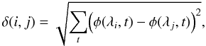 (1)where
 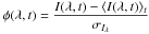 represents the standardised irradiance at wavelength λ, ⟨ · ⟩ t expresses time averaging, and σIλ is the standard deviation of the considered irradiance. When the data are highly correlated, as is the case here, then they can be represented reasonably well on a 2D map, while letting their pairwise distance reflect their dissimilarity. The idea is thus to project our multidimensional cloud of wavelengths on a 2D subspace that captures their salient properties in terms of distances. A better known example of multidimensional scaling is reconstructing a map of a country according to distances between all pairs of cities.
Interestingly, the location of all the points on the 2D map can be readily obtained from only a few matrix operations, using the Singular Decomposition Method (SVD) (Golub & Van Loan 2000). This technique decomposes the normalised irradiances into sets of separable functions of time and wavelength 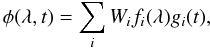 (2)with the condition that these functions are orthonormal, i.e.,
 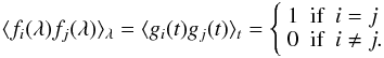 (3)Each weight squared
  represents the amount of variance that is described by the ith dimension. Weights are conventionally sorted in decreasing order. Here, the first weights carry a major fraction of the variance thanks to the remarkable redundancy of solar spectral variability. This justifies in principle the projection of all wavelengths on a low-dimensional subspace where the coordinates of each wavelength along the ith dimension (axis) is simply given by Wifi(λ). The major advantage of this approach is that the dissimilarity between all wavelengths and passbands can be evaluated at a single glance. Doing the same by means of the more classical tables of pairwise correlation coefficients would be intractable.
Different time scales in the solar variability also express different physical mechanisms. To explore this in more detail, we built two data sets, a lowpass and a highpass one, with a cutoff at 81 days (using a Butterworth filter). This cutoff of three solar rotation periods approximately corresponds to the lifetime of active regions. High- and low-pass data respectively capture rapid variations and solar rotation effects, and slow variations, including the solar cycle.
In what follows, we first normalise the data and subsequently filter them before applying the multidimensional scaling. For the sake of comparison, two of the most widely used UV indices, namely the F10.7 and the MgII indices, are included in the analysis.
3.1. Long time scales
Let us first consider the lowpass filtered data, which describe the long-term evolution of the solar spectral irradiance on scales of several months and beyond. The first three projections obtained by SVD respectively capture 96%, 2%, and 1%of the variance. From this we readily conclude that the salient features are properly described by a 2D and even by a 1D projection. This is not surprising since the long term evolution is very similar at all wavelengths and also in the two solar indices.
Figure 1 presents the 2D map. Adding more dimensions does not give deeper insight and merely complicates the visualisation. Neither the meaning of the axes nor the units are important here; what does matter is the relative distance between the points, each of which corresponds to a wavelength bin, a passband, or an index. This distance directly reflects the degree of dissimilarity between the variability between corresponding points. In a forthcoming paper, we shall elaborate on the physical interpretation of these projections. In Fig. 1, most of the scatter occurs along the vertical axis. Most wavelengths are grouped in one single cluster, and the only outliers are some wavelengths in the 45–70 nm range, which are known to suffer from instrumental artefacts associated with degradation. The ten passbands are represented in Fig. 1 by a letter coding, see Table 1. As expected, all passbands are located within the main cluster of points, except for PREMOS 2 (P2), which coincides with the spectral band it is supposed to describe. The F10.7 and MgII indices are clearly located outside of the cluster of points, so even though they are reasonably good indices, better performance can achieved here by using passbands. This is precisely the reason for advocating a reconstruction from a few passbands rather than from indices.
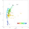 |
Fig. 1 2D representation of the normalised fluxes for long time scales. Colour codes correspond to wavelengths (nm). Passbands and indices are indicated by letters (see Table 1). The two axes correspond to Wifi(λ). |
It is worth mentioning that any linear combination of two nearby passbands will be located approximately on a straight line passing through them. As an example, we included in the analysis the average of PREMOS 2 and EUV B, giving the red point “H” in Fig. 1. One can check that this point is indeed located half way between “P2” and “B”. From Fig. 1, we can now propose a strategy for selecting the best passbands: they should be located as close as possible to the different wavelengths while being distributed all over the cluster. In addition to this, linear combinations of passbands (i.e. lines linking pairs of passbands) should cover the clusters. We conclude from Fig. 1 that any of the passbands (except PREMOS 2) can be used for reconstructing the long-term variability in the EUV and FUV, since their long-term evolutions are very similar. In particular, there is no compelling reason for distinguishing emissions originating in the corona (as measured as EUV A-D, LYRA Al, and LYRA Zr) or emissions from lower layers, as provided by LYRA Ly and EUV E. These two passbands exhibit a different behaviour because LYRA Ly has a strong contribution of wavelength longward of 130 nm, while EUV E is a narrow filter centred on the bright Lyman-α line. A rapid estimation actually shows that the scatter of these passbands on the 2D map is within the instrumental error bars of the data from the different instruments. In the MUV range, PREMOS 2 is recommended for wavelengths longer than 230 nm, so depending on the range that needs to be reconstructed and the desired accuracy, one can use either one passband only for the EUV & FUV or two for the whole UV spectrum. There is no need to have more of them.
Besides the choice of the passbands, other criteria require consideration when designing a radiometer measuring the UV irradiance. The detector technology is one of them. Detectors using silicon technology exhibit some drawbacks, especially the high sensitivity to visible light or the signal contamination due to the low-working temperature of the detectors needed to limit the noise. Wide band gap materials, such as diamond, cubic boron nitride, and aluminium nitride, would definitely help to circumvent these limitations of silicon detectors (Hochedez et al. 2000). In contrast to silicon, diamond detectors (with a gap potential Eg ≈ 5.5 eV at room temperature) are “solar-blind” with an UV/Visible rejection ratio of at least four orders of magnitude. Because they are less subject to pinhole degradation and more radiation hard, diamond detectors should also present a longer lifetime than silicon detectors making them a priori suitable for space weather missions. The LYRA and PREMOS detectors use diamond technology, so when in the following some passbands are found to be equivalent, we prefer these diamond detectors. To reconstruct the long-term variability of the UV solar spectrum, we propose LYRA Ly and PREMOS 2 for the following.
To check this strategy, we compared two reconstructions of the solar spectrum, one that is based on above-mentioned pair of channels and another based on a combination of pass bands that offers the best coverage of the entire spectrum (Lyra Al, LYRA Ly, LYRA Hb, and PREMOS 2). The results are very similar, which supports the validity of our statistical approach and also points out that it is unnecessary to entirely cover the solar spectrum with different passbands in order to capture the spectral variability. Only a few passbands (here two) are needed to capture the salient properties of the long-term spectral variability. It must be stressed, however, that these conclusions are only based on the last six years of data, and so one should be cautious in extrapolating them to future solar cycles. Future measurements of the full UV spectrum will tell us how our empirical models stand the test of time.
3.2. Short time scales
Short time scales capture time scales below 81 days and thus mostly reflect the variability associated with solar rotation. The first three weights of the SVD method respectively capture 82%, 8%, and 4% of the variance. The coherency of the spectral variability is not as strong anymore as with the long-term evolution, as was to be expected from the properties of the EUV/FUV/MUV spectrum. In spite of this, a 2D map still captures over 90% of the variance and thus represents the relative distances relatively well between the spectral lines. This map is shown in Fig. 2. In contrast to Fig. 1, we now see a clear structuring according to the wavelength along the vertical axis, with the hot coronal lines at the top, while most chromospheric and transition region lines are at the bottom. Wavelengths above 180 nm are clustered differently along the horizontal axis. A finer analysis of the first two functions of time gi(t) reveals that the horizontal axis represents the modulation amplitude on a 27-day solar period, while the vertical axis captures the 13.5-day modulation amplitude, which is a signature for center-to-limb variations. The F10.7 index remains outside of the cloud of points, which again illustrates the superior performance of passbands.
In contrast to the long-term scales, passbands are no longer located within a unique cluster. As in Fig. 1, the passbands coincide with the spectral bands they are supposed to describe. Based on the strategy developed in Sect. 3.1, we can define the most appropriate set of passbands for reconstructing the short-term variability. According to Fig. 2, the next six candidates exhibit very similar time evolutions: LYRA Al, LYRA Zr, and the four spectral bands from EUVS (EUV A-D). Only one is needed approximately to reconstruct the five others. LYRA Al could be an excellent choice since the spectral band of this particular channel includes He II at 30.4 nm, but also uses diamond technology. Finally LYRA Al, combined with LYRA Ly, LYRA Hb, and PREMOS 2, will provide excellent coverage of the 2D map. These four filters are therefore recommended for reconstructing the short term variability of the solar UV spectrum. This leads us to distinguish emissions coming from the corona (as measured by EUV A-D, LYRA Al, and LYRA Zr) from emissions coming from lower layers (as provided by LYRA Ly and EUV E). We checked the performance of all 210 combinations of four passbands out of ten and our choice indeed comes out as one of the very few combinations that minimises the reconstruction error (to be discussed below).
4. Reconstruction method
Our empirical model for reconstructing the UV spectrum is based on a linear combination of the response of the passbands (Fi): 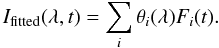 (4)One model is built for fitting the long-term evolution, and a different one is for the short-term evolution. The fitting capacity of these models can in principle be augmented by including more regressors, with for example a constant term, or nonlinear combinations of the fluxes. We found, however, that the resulting improvement in the reconstruction was not significant as compared to the inherent uncertainty of the data. A convenient measure of the quality of the reconstruction is the relative error, which is defined as
 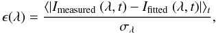 (5)where σλ is again the standard deviation of Imeasured (λ,t). This estimate gives values that are considerably higher than the ones obtained from the more conventional definition, in which a normalisation versus the average value is used. Our choice is motivated by the need for reconstructing the spectral variability and not just the average spectral irradiance.
We estimate the model parameters (θi) by using a least-squares method and compute the relative error on different time intervals. The model is trained on a sample of 600 days (including both solar maximum and solar minimum) and then tested on the remaining 1600 days (see Fig. 5).
We now look at the reconstruction based on the response from passbands, on one hand, and on indices (F10.7 and Mg II), on the other. As mentioned before, we do not investigate the 210–230 nm range.
4.1. Long time scales
We first consider the reconstruction for long time scales. Using the result from Sect. 3.1, we use the passbands LYRA Ly and PREMOS 2 for reconstructing the long-term variability. The relative error is displayed in Fig. 3; also shown is the relative error obtained by using only the Mg II and F10.7 indices only. The two passbands suffice for reconstructing the long-term variability of the UV solar spectrum with a relative error of about 20%. While PREMOS 2 is definitely required for the MUV range, any of the other passbands can be used for reconstructing the EUV & FUV ranges with a similar relative error. Their performance is definitely better than for the indices alone.
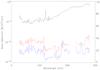 |
Fig. 3 Relative error for the long time scale versus wavelength (nm) for the set of passbands (LYRA Ly and PREMOS 2 in blue), and for the reconstruction based on two indices (Mg II and F10.7, in red). The solar spectrum is shown for comparison in black, with 1-nm resolution. |
4.2. Short time scales
For short time scales, we use the set of passbands that minimises the relative error on the reconstruction of the short-term variability: LYRA Al, LYRA Ly, LYRA Hb, and PREMOS 2. The relative error for the four passbands and the two indices, are displayed in Fig. 4. Let us stress that the F10.7 and MgII indices are not surrogates for the MUV range, so a better gauge for photospheric emissions is needed, which explains the dramatic increase in the relative error for wavelengths above 180 nm. By using the passbands, the short-term variability of the UV solar spectrum can be reconstructed with a relative error of about 20% for the FUV and MUV ranges. Some wavelengths in the EUV range, however, are more difficult to reconstruct.
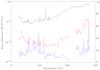 |
Fig. 4 Relative error for the short time scales versus wavelength (nm) for a model based on four passbands described in Sect. 4.2 (in blue), and for the reconstruction based on two indices (in red). The solar spectrum is shown for comparison in black, with a 1-nm resolution. |
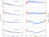 |
Fig. 5 Comparison between the measured (in black) and the fitted (in colour) irradiances, for four wavelengths on the left and their residual on the right. The measurement precision (4% for SEE, 1% for SOLSTICE) is indicated in each plot. The fit is based on the set of passbands described in the text. The model parameters are estimated from the maximum and the minimum of the solar cycle (in red), while the relative error is estimated within the blue interval, which corresponds approximatively to 1600 days. |
5. Total reconstruction
We now combine the models for the long and the short time scales to reconstruct the full spectral irradiance. The set of passbands we use is the same as before: LYRA Ly and PREMOS 2 for long time scales and LYRA Al, LYRA Ly, LYRA Hb, and PREMOS 2 for short time scales. Both LYRA Al and LYRA Hb are unnecessary for the reconstruction of the long time scale since their temporal behaviour is redundant with LYRA Ly. The results are summarised in Fig. 5, which displays four typical wavelength bins and their reconstruction, with the residual error (i.e. the difference between the two). The irradiance in the 30.5 nm bin is dominated by the He II line at 30.34 nm with a significant contribution from coronal lines. The 121.5 nm bin represents the strong Lyα line, which is very well reconstructed. The two other bins represent the contribution of the Si II at 181.69 nm and the Mg I absorption edge at 251 nm. The 27-day modulation is properly reconstructed as expected, while one can notice a slight discrepancy (less than 1%) over the long term for wavelength in the MUV range. According to this study, four passbands suffice for reconstructing the solar variability in the UV range with a relative error of about 20%. However, several wavelengths in the 40–70 range remain difficult to reconstruct. This was to be expected because these bins are also located away from the clusters in Figs. 1 and 2. The main raison for this is probably the instrument degradation, which causes long-term drifts.
The definition of a set of passbands dedicated to monitoring the UV solar spectrum is not unique. The statistical strategy developed here allows defining several sets of passbands that could give similar results.
The model parameters (θi) here depend directly on the instrument EGS/TIMED and SOLSTICE/SORCE data, which are the only spectral irradiance measurements that are available for the whole UV spectrum. The quality of the reconstruction should therefore be linked to the quality of the inputs data. The key figure here is the absolute accuracy of the measurements: 10–20% for EGS and 1.2–6% for SOLSTICE, where our reconstruction is as good as the spectral irradiances inputs are. Besides, the model parameters depend directly on the chosen passbands. A full characterisation of the responsitivities of the chosen channels is therefore required to compute the appropriate model parameters. Next comes the problem of the degradation of the passbands, including changes in the spectral responsivities. Few studies have been done in the past, and the degradation is often modelled by an empirical law (e.g. Floyd 1999). The chosen passbands should exhibit minor degradation or at least a degradation that can easily be modelled to adjust the model parameters. The choice of the technologies of filters and detectors is also a major criterion. A radiometer dedicated to the space weather should be as robust as possible to allow long-term monitoring. Diamond detectors should thus be an excellent choice and, LYRA will certainly provide information about the longevity of these detectors.
6. Conclusions
We have investigated here how the solar spectral variability in the EUV/FUV/MUV bands (for time scales of days and beyond) can be reconstructed empirically from the linear combination of the observations made in a few spectral bands. To do so, we first simulated the response of ten existing detectors with different passbands, using six years of daily measurements of the UV spectrum from SORCE and TIMED. Next, we proposed a strategy for determining the best combination of detectors, using a graphical representation based on multidimensional scaling. We identified several key spectral ranges from a statistical point of view and for a non-flaring Sun at a resolution of 1 nm.
This work points out that it is unnecessary to entirely cover the solar spectrum with different passbands in order to reconstruct the spectral variability at all wavelengths. Some non-overlapping passbands give very similar responses that are well within the experimental error of the instruments. This is a manifestation of a few degrees of freedom in the solar spectral variability. As a consequence of this, the UV spectrum can be reconstructed between 27 and 280 nm using only four passbands and with a relative error of about 20%. The error obtained by reconstructing the spectrum only from solar indices, such as F10.7 and Mg II, is about two times larger. Direct observations of a few passbands therefore bring a major improvement to spectral reconstructions, as compared to proxy-based reconstructions. However, we must stress that this study is only based on six years of observations. So at least one full solar cycle is needed to validate it.
As an outcome of this study, we are now using the four channels of LYRA/PROBA2 to reconstruct the solar spectral variability in nearly real time. The recent launch of the Extreme ultraviolet Variability Experiment (EVE) onboard Solar Dynamics Observatory (SDO) (Woods et al. 2010) will provide an opportunity to extend our study to the XUV range and with a subminute cadence. As no observation of the full UV spectrum will exist after the SORCE missions ends, the method presented here will be useful for filling spectral gaps. Finally, this study paves the way for a simple instrumental concept that could be used for monitoring the solar UV spectrum in the framework of the Space Situational Awareness programme.
Acknowledgments
This study received funding from the European Community’s Seventh Framework Programme (FP7/2007-2013) under the grant agreement No. 218816 (SOTERIA project, www.soteria-space.eu). The authors wish to thank the anonymous referee for his careful reading of the manuscript and his fruitful comments and suggestions.
References
- Amblard, P., Moussaoui, S., Dudok de Wit, T., et al. 2008, A&A, 487, L13 [NASA ADS] [CrossRef] [EDP Sciences] [Google Scholar]
- Busá, I., Andretta, V., Gomez, M. T., & Terranegra, L. 2001, A&A, 373, 993 [NASA ADS] [CrossRef] [EDP Sciences] [Google Scholar]
- Chamberlin, P. C., Woods, T. N., & Eparvier, F. G. 2008, Space Weather, 6, 5001 [CrossRef] [Google Scholar]
- Chatfield, C., & Collins, A. J. 1990, Introduction to Multivariate Analysis (London: Chapman & Hall) [Google Scholar]
- Crane, P. C., Floyd, L. E., Cook, J. W., et al. 2004, A&A, 419, 735 [NASA ADS] [CrossRef] [EDP Sciences] [Google Scholar]
- Domingo, V., Ermolli, I., Fox, P., et al. 2009, Space Sci. Rev., 145, 337 [Google Scholar]
- Dudok de Wit, T., Kretzschmar, M., Lilensten, J., & Woods, T. 2009, Geophys. Res. Lett., 36, 10107 [NASA ADS] [CrossRef] [Google Scholar]
- Dudok de Wit, T., Lilensten, J., Aboudarham, J., Amblard, P., & Kretzschmar, M. 2005, Ann. Geophys., 23, 3055 [NASA ADS] [CrossRef] [Google Scholar]
- Egorova, T., Rozanov, E., Manzini, E., et al. 2004, Geophys. Res. Lett., 31, 6119 [NASA ADS] [CrossRef] [Google Scholar]
- Evans, J. S., Strickland, D. J., Woo, W. K., et al. 2010, Sol. Phys., 262, 71 [Google Scholar]
- Feldman, U., Brown, C. M., Seely, J. F., et al. 2010, J. Geophys. Res., Space Phys., 115, 3101 [CrossRef] [Google Scholar]
- Fineschi, S., & Viereck, R. A. 2007, Solar Physics and Space Weather Instrumentation II, SPIE Conf. Ser., 6689 [Google Scholar]
- Floyd, L. 1999, Adv. Space Res., 23, 1459 [Google Scholar]
- Floyd, L., Newmark, J., Cook, J., Herring, L., & McMullin, D. 2005, J. Atm. Solar-Terrestrial Phys., 67, 3 [Google Scholar]
- Golub, G. H., & Van Loan, C. F. 2000, Matrix Computations, ed. J. H. Press (Baltimore) [Google Scholar]
- Gray, L. J., Beer, J., Geller, M., et al. 2010, Rev. Geophys., 48, RG4001 [Google Scholar]
- Heath, D. F., & Schlesinger, B. M. 1986, J. Geophys. Res., 91, 8672 [NASA ADS] [CrossRef] [Google Scholar]
- Higgins, P. A., Gallagher, P. T., McAteer, R. T. J., & Bloomfield, D. S. 2010, Adv. Space Res., in press [arXiv:1006.5898] [Google Scholar]
- Hinteregger, H. E. 1981, Adv. Space Res., 1, 39 [Google Scholar]
- Hochedez, J., Schmutz, W., Stockman, Y., et al. 2006, Adv. Space Res., 37, 303 [NASA ADS] [CrossRef] [Google Scholar]
- Hochedez, J., Verwichte, E., Bergonzo, P., et al. 2000, Phys. Stat. Sol. Appl. Res., 181, 141 [NASA ADS] [CrossRef] [Google Scholar]
- Kretzschmar, M., Lilensten, J., & Aboudarham, J. 2004, A&A, 419, 345 [NASA ADS] [CrossRef] [EDP Sciences] [Google Scholar]
- Kretzschmar, M., Lilensten, J., & Aboudarham, J. 2006, Adv. Space Res., 37, 341 [Google Scholar]
- Kretzschmar, M., Dudok de Wit, T., Lilensten, J., et al. 2008, Acta Geophys., 57, 42 [NASA ADS] [CrossRef] [Google Scholar]
- Krivova, N. A., & Solanki, S. K. 2008, J. Astrophys. Astron., 29, 151 [NASA ADS] [CrossRef] [Google Scholar]
- Lean, J. 1987, J. Geophys. Res., 92, 839 [NASA ADS] [CrossRef] [Google Scholar]
- Lean, J. L., Livingston, W. C., Heath, D. F., et al. 1982, J. Geophys. Res., 87, 10307 [NASA ADS] [CrossRef] [Google Scholar]
- Lean, J. L., Warren, H. P., Mariska, J. T., & Bishop, J. 2003, J. Geophys. Res., Space Phys., 108, 1059 [Google Scholar]
- Lilensten, J., Dudok de Wit, T., Kretzschmar, M., et al. 2008, Ann. Geophys., 26, 269 [NASA ADS] [CrossRef] [Google Scholar]
- Richards, P. G., Fennelly, J. A., & Torr, D. G. 1994, J. Geophys. Res., 99, 8981 [Google Scholar]
- Richards, P. G., Woods, T. N., & Peterson, W. K. 2006, Adv. Space Res., 37, 315 [Google Scholar]
- Rottman, G. 2005, Sol. Phys., 230, 7 [NASA ADS] [CrossRef] [Google Scholar]
- Schmidtke, G., Tobiska, W. K., & Winningham, D. 2002, Adv. Space Res., 29, 1553 [NASA ADS] [CrossRef] [Google Scholar]
- Shapiro, A. I., Schmutz, W., Schoell, M., Haberreiter, M., & Rozanov, E. 2010, A&A, 517, A48 [NASA ADS] [CrossRef] [EDP Sciences] [Google Scholar]
- Snow, M., McClintock, W. E., Rottman, G., & Woods, T. N. 2005, Sol. Phys., 230, 295 [NASA ADS] [CrossRef] [Google Scholar]
- Tapping, K. F., & Detracey, B. 1990, Sol. Phys., 127, 321 [Google Scholar]
- Thuillier, G., Dewitte, S., Schmutz, W., & The Picard Team 2006, Adv. Space Res., 38, 1792 [NASA ADS] [CrossRef] [Google Scholar]
- Tobiska, W., & Nusinov, A. 2006, in COSPAR, Plenary Meeting, 36, 36th COSPAR Scientific Assembly, 2621 [Google Scholar]
- Tobiska, W. K., Woods, T., Eparvier, F., et al. 2000, J. Atm. Solar-Terrestrial Phys., 62, 1233 [Google Scholar]
- Vourlidas, A., Klimchuk, J. A., Korendyke, C. M., Tarbell, T. D., & Handy, B. N. 2001, ApJ, 563, 374 [NASA ADS] [CrossRef] [Google Scholar]
- Warren, H. P., Mariska, J. T., & Lean, J. 1998, J. Geophys. Res., 103, 12077 [NASA ADS] [CrossRef] [Google Scholar]
- Woods, T. N., Eparvier, F. G., Bailey, S. M., et al. 2005, J. Geophys. Res., Space Phys., 110, 1312 [Google Scholar]
- Woods, T. N., Kopp, G., & Chamberlin, P. C. 2006, J. Geophys. Res., Space Phys., 111, 10 [Google Scholar]
- Woods, T. N., Chamberlin, P. C., Peterson, W. K., et al. 2008, Sol. Phys., 250, 235 [NASA ADS] [CrossRef] [Google Scholar]
- Woods, T. N., Eparvier, F. G., Hock, R., et al. 2010, Sol. Phys., 3 [Google Scholar]
- Worden, J. R., White, O. R., & Woods, T. N. 1998, ApJ, 496, 998 [Google Scholar]
All Tables
List of the passbands (with their letter code) used in this study and their spectral range.
All Figures
|
Fig. 1 2D representation of the normalised fluxes for long time scales. Colour codes correspond to wavelengths (nm). Passbands and indices are indicated by letters (see Table 1). The two axes correspond to Wifi(λ). |
| In the text | |
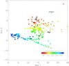 |
Fig. 2 Same plot as Fig. 1, for short time scales (<81 days). |
| In the text | |
|
Fig. 3 Relative error for the long time scale versus wavelength (nm) for the set of passbands (LYRA Ly and PREMOS 2 in blue), and for the reconstruction based on two indices (Mg II and F10.7, in red). The solar spectrum is shown for comparison in black, with 1-nm resolution. |
| In the text | |
|
Fig. 4 Relative error for the short time scales versus wavelength (nm) for a model based on four passbands described in Sect. 4.2 (in blue), and for the reconstruction based on two indices (in red). The solar spectrum is shown for comparison in black, with a 1-nm resolution. |
| In the text | |
|
Fig. 5 Comparison between the measured (in black) and the fitted (in colour) irradiances, for four wavelengths on the left and their residual on the right. The measurement precision (4% for SEE, 1% for SOLSTICE) is indicated in each plot. The fit is based on the set of passbands described in the text. The model parameters are estimated from the maximum and the minimum of the solar cycle (in red), while the relative error is estimated within the blue interval, which corresponds approximatively to 1600 days. |
| In the text | |
Current usage metrics show cumulative count of Article Views (full-text article views including HTML views, PDF and ePub downloads, according to the available data) and Abstracts Views on Vision4Press platform.
Data correspond to usage on the plateform after 2015. The current usage metrics is available 48-96 hours after online publication and is updated daily on week days.
Initial download of the metrics may take a while.