| Issue |
A&A
Volume 528, April 2011
|
|
|---|---|---|
| Article Number | A44 | |
| Number of page(s) | 7 | |
| Section | Stellar atmospheres | |
| DOI | https://doi.org/10.1051/0004-6361/201015814 | |
| Published online | 28 February 2011 | |
Research Note
Microturbulent velocity from stellar spectra: a comparison between different approaches
Dipartimento di AstronomiaUniversitá degli Studi di Bologna,
via Ranzani 1,
40126
Bologna,
Italy
e-mail: alessio.mucciarelli2@unibo.it
Received: 24 September 2010
Accepted: 17 January 2011
Context. The classical method to infer microturbulent velocity in stellar spectra requires that the abundances of the iron lines are not correlated with the observed equivalent widths. An alternative method, requiring the use of the expected line strength, is often used to bypass the risk of spurious slopes caused by the correlation between the errors in abundance and equivalent width.
Aims. Our aim is to compare the two methods, describe their respective advantages and disadvantages, and show how they apply to the typical practical cases.
Methods. We performed a test with a grid of synthetic spectra, including instrumental broadening and Poissonian noise. For these spectra, we derived the microturbulent velocity by using the two approaches and compared the results with the original value with which the synthetic spectra were generated.
Results. The two methods provide similar results for spectra with SNR ≥ 70, while for lower signal-to-noise (SNR) both approaches underestimate the true microturbulent velocity, depending on the SNR and the possible selection of the lines based on the equivalent width errors. Basically, the values inferred by using the observed equivalent widths better agree with those of the synthetic spectra. Indeed, the method based on the expected line strength is not totally free from a bias that can heavily affect the determination of microturbulent velocity. Finally, we recommend to use the classical approach (based on the observed equivalent widths) to infer this parameter. For a full spectroscopical determination of the atmospherical parameters, the difference between the two approaches is reduced, which leads to an absolute difference in the derived iron abundances of less than 0.1 dex.
Key words: stars: fundamental parameters / techniques: spectroscopic
© ESO, 2011
1. Introduction
One of the major limitations in the model atmospheres based on 1D geometry is an unrealistic treatment of the surface convection. Usually, the convective energy transfer is computed by adopting the classical mixing-length theory (Böhm-Vitense 1958), a parameterization aimed to bypass the lack of a rigorous mathematical formulation for the convective energy transfer. On the other hand, this parameterization cannot describe the convective phenomena realistically, because it ignores their time-dependent and non-local nature.
Basically, photospheric turbulent motions are divided into two typologies, according to the size of the turbulent element: if this is smaller than the mean free path of the photons, we call it microturbulence, if it is larger, macroturbulence.
These motions broaden the spectral lines, and the necessity to parameterize these effects arises from the discrepancy between the empirical and theoretical curves of growth (COG) on their flat part. Microturbulent velocity (hereafter vt) is a free parameter introduced to remove this discrepancy and to compensate for the missing broadening. Usually, vt is included during the spectral synthesis in the Doppler shift calculation, adding in quadrature vt and thermal Doppler line broadening.
Some general objections can be voiced against on this simplification:
-
(1)
the distinction between micro and macroturbulence is only anarbitrary boundary, because it is based on the incorrectassumption that the velocity fields work on a discrete scale, whilethese velocity fields rather run on a continuous scale;
-
(2)
the 1-D model atmospheres (usually adopted in the chemical analysis) include depth-independent microturbulent velocity. Observational hints point toward a different scenario, see e.g. the works about Arcturus by Gray (1981) and Takeda (1992);
-
(3)
the turbulent velocity distribution is generally modeled as isotropic and Gaussian; this is contradicted by the observation of the granulation on the solar surface; as pointed out by Nordlund et al. (1997) and Asplund et al. (2000), the phenomenon of photospheric granulation is characterized by laminar (and not turbulent) velocities, caused by strong density stratification;
-
(4)
the mixing-length theory describes the general temperature structure of the photosphere, but it is unable to model some relevant convective effects, such as the photospheric velocity field and the horizontal fluctuations in the temperature structure (Steffen & Holweger 2002).
The classical and empirical way to estimate vt is to erase any slope between the abundance A(Fe)1 and the reduced equivalent width log 10(EW/λ) (hereafter EWR, where EW is the equivalent width), because vt preferentially works on the moderated/strong lines, while the weak ones are more sensitive to abundance. Even if the least-square fitting of these two quantities is usually used to infer vt, this method requires that the two quantities have uncorrelated errors. This condition is not met in this case, because the errors in EWR and A(Fe) are obviously correlated, with the risk to introduce a spurious slope in the A(Fe)–EWR plane.
To bypass this obstacle and provide a more robust diagnostic to infer vt, Magain (1984) proposed to derive vt by using the theoretical EW (hereafter EWT) instead of the observed one. In this paper, we investigate the impact of these two approaches to derive vt, in order to evaluate their reliability and to estimate the best one to use in the typical chemical abundance analysis.
2. Artificial spectra: general approach
The basic idea is to generate sets of synthetic spectra with a given and a priori known vt (with inclusion of instrumental broadening and noise) and to analyze them with the two methods. Such a procedure allows one to estimate the absolute goodness of the two methods (comparing the derived vt with the original one) but also the relative accuracy between the two approaches to highlight systematic effects, if any.
Different sets of artificial spectra were generated with the following method:
-
(1)
synthetic spectra for a giant star withTeff = 4500 K, log g = 2.0, [M/H] = –1.0 dex and vt = 2 km s-1 were computed with the spectro-synthesis code SYNTHE by Kurucz in its Linux version (Sbordone et al. 2004, 2005), starting from LTE, plane-parallel ATLAS 9 model atmospheres and by adopting the line compilation by Kurucz2; the synthetic spectra cover a wavelength range between 5500 and 8000 Å;
-
(2)
the spectra were convolved with a Gaussian profile to mimic the instrumental resolution of the modern echelle spectrographs. A spectral resolution of λ/δλ = 45 000 was adopted (analogous to that of several spectrographs as UVES, CRIRES, SARG);
-
(3)
the broadened spectra were re-sampled to a constant wavelength step of δx = 0.02 Å/pixel (similar to that of UVES echelle spectra);
-
(4)
poissonian noise was added to the rebinned spectra by using the IRAF task MKNOISE to reproduce different noise conditions. Signal-to-noise (SNR) ratios of 25, 40, 50, 70, 100 and 200 were simulated. Owing to the random nature of the noise, we resorted to MonteCarlo simulations, and for each value of SNR, 200 artificial spectra were generated and analyzed independently.
We selected from the Kurucz linelist ~250 Fe I transitions in the spectrum, taking into account only unblended lines or those with negligible blending, similarly to what is done on real observed spectra. For all spectra, EWs were measured with the automatic code DAOSPEC (Stetson & Pancino 2008).
3. Determination of vt and caveats
For all synthetic spectra described above, least-square fits were computed both in the A(Fe)–EWR and A(Fe)–EWT planes, choosing the value of vt that minimizes the slope. All other parameters (Teff, log g and [M/H]) were kept fixed, according to the original ones of the synthetic spectra3.
The most often adopted proxy for the theoretical line strength can be written as log 10(gf) − θχex (see also Eq. (14.4) in Gray 1992), where log 10(gf) is the oscillator strength, θ the Boltzmann factor (defined as θ = 5040/Teff) and χex the excitation potential. Note that EWT does not include terms strictly inferred by the observations but only those related to the adopted model atmospheres (θ) and to atomic data of the involved transitions (log 10(gf) and χex).
Figure 1 shows the comparison between the true equivalent width computed for the synthetic spectrum of the giant star (before adding noise) and the proxy used for EWT. It is evident from the figure that the quantity log 10(gf) − θχex is proportional to the true equivalent width of the synthetic spectrum (at least in the EW range shown in Fig. 1), because it is a monotonic function of the true EW. In this work, we adopt the quantity log 10(gf) − θχex as the proxy for EWT because this is the formalism usually adopted in the chemical analysis that follow the method described by Magain (1984).
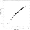 |
Fig. 1 Behavior of the true equivalent widths measured in the synthetic spectrum (without Poissonian noise) computed with the atmospheric parameters of a giant star, as a function of the quantity log 10(gf) − θχex. |
A threshold for the strongest lines was applied: only lines weaker than log (EW/λ) = –4.85 were included in the analysis, corresponding to ~78 m Å at 5500 Å and ~113 m Å at 8000 Å. Stronger lines (basically located along the flat/damped part of the COG) were excluded in order to avoid additional effects (both observational and theoretical) that could affect the determination of vt. In fact: (i) strong features deviate from the Gaussian approximation (owing to the development of Lorenztian wings), with the risk to underestimate the EW (as discussed in Stetson & Pancino 2008, see their Fig. 7); and (ii) these lines are affected by other effects, in addition to the microturbulent velocity, i.e. hyperfine/isotopic splitting, damping treatment and modeling of outermost atmospheric layers: the inclusion of these lines could lead to a different vt, which is very sensitive to the treatment of these effects for the iron lines, but it is not sure that the derived vt will be appropriate also for other elements (as discussed by Ryan 1998). Generally stronger lines can be taken into account in the abundance analysis (and for some elements like Ca or Ba only strong/damped transitions are often available), but they should be excluded from the determination of vt.
We recall that the approach used in this work represents only a simple case compared with the analysis of real spectra, because it is based on some simplifications:
-
(i)
the large number of unblended lines. In real spectra, the numberof lines is limited by the quality of the available oscillatorstrengths and by the wavelength coverage;
-
(ii)
only vt is adopted as a free parameter to determine, because the other atmospherical parameters are known before from the computation of the synthetic spectra;
-
(iii)
the used spectra are flat and their continuum (virtually) set to the unity. Hence, distortions of the continuum caused by residual fringing, uncorrected merging of the echelle orders or the residual of blaze function are not included;
-
(iv)
this analysis is limited to features that can be well reproduced by a Gaussian function, while in real cases some features with prominent damping wings can be included in the analysis by adopting a Voigt profile fitting (but taking into account the caveats discussed above for strong lines).
4. Impact of the SNR
For each SNR, 200 artificial spectra were generated and analyzed independently, and the mean value of vt of each group of SNR was derived. An important step in this kind of analysis is a careful selection of the lines used to infer vt, excluding features not well measured that could introduce a bias in the vt determination. In order to quantify the impact of inaccurate EWs in the vt estimate, we determined vt by considering different error thresholds and by taking into account only lines with errors σEW less than 10, 20, 30, and 50%; these errors were computed by the DAOSPEC code from the standard deviation of the local flux residuals and represent a 68% confidence interval on the derived value of the EW (see Stetson & Pancino 2008, for details). The discarding of lines with inaccurate EWs was performed individually for each artificial spectrum. As sanity check, the EWs measured in a synthetic spectrum with SNR = 25 were compared with the true EWs of the original spectrum (before adding noise). The results are shown in Fig. 2; the inner panels show the behavior of the relative error in percentage as a function of the true and measured EW (left and right inset, respectively). These plots confirm the reliability of the measured EWs and show that the errors in the EW measurement mainly affect the weak lines, while the strong ( > 40 mÅ) lines are well measured with small uncertainties.
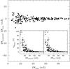 |
Fig. 2 Difference between the measured and true EW in a synthetic spectrum with SNR = 25 as a function of the true EW. In the left inset we show the behavior of the error in percentage of the measured EW as a function of the true EW, while in the right inset we show the same behavior as a function of the measured EW. |
The results concerning the determination of vt with the two methods for the sample of synthetic spectra described above are plotted in Fig. 3, where empty and filled circles indicate the values of vt derived by using the EWR and EWT method, respectively. The errorbars indicate the dispersion around the mean of each set of simulations of a given SNR. For sake of clarity, the original value of vt of the synthetic spectra is plotted as a dashed line. Typically, the dispersion around the mean in each group ranges from a few hundredths of km s-1 (for SNR = 100 and 200) up to 0.2 km s-1 for SNR = 25 and considering lines with residual errors less than 50%; note that these dispersions are basically compatible with the corresponding errors of the computed slopes4.
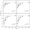 |
Fig. 3 Behavior of the measured microturbulent velocity as a function of SNR, derived with the classical method (empty circles) and the prescription by Magain (1984) (filled circles) for a giant star. Each point is the average value obtained by using 200 synthetic spectra of a given SNR, and the errorbars indicate the dispersion around the mean. Dashed lines indicate the original value of vt of the synthetic spectra. Each panel shows the results obtained by considering different thresholds for the residual errors in the EW measurement. |
For relatively high ( ≥ 70) SNR, the two methods provide very similar results and agree with the vt of the original synthetic spectrum. Indeed, if the SNR is increased, the errors in the EW measurements are reduced and the discrepancy between the two approaches is erased. On the other hand, spectra with SNR < 70 show vt always lower than the original value , and the discrepancy increases when lines with high uncertainties are also taken into account. Generally vt inferred by using EWT turns out to be systematically lower than that obtained with the classical method by 0.1–0.2 km s-1, approximately. The reasons of this systematic underestimate will be explained in Sect. 5.
These findings also highlight the impact of measured EWs with high uncertainties: the inclusion of lines with very uncertain EWs (generally, the weakest lines in spectra with low SNR) worsens the discrepancy with the true vt of the original synthetic spectra. Thus, a careful selection of the used lines, considering the accuracy of their EWs, is crucial in the derivation of vt to exclude additional bias.
A simple analytical model can be derived by fitting the data shown in Fig. 3. The absolute value δvt of the difference between the derived vt and the true one can be expressed as δvt = fσEW/SNR, where fσEW is a linear function of the adopted error threshold σEW (expressed in %). The fit of the present dataset provides δvt = (0.14·σEW + 2.64)/SNR for vt derived by using EWR and δvt = (0.19·σEW + 5.16)/SNR when EWT is adopted.
We also repeated these checks with synthetic spectra computed with the typical parameters of a dwarf star (Teff = 6000 K, log g = 4.0, [M/H] = –1.0 dex and vt = 1 km s-1), finding basically the same result.
5. Is the EWT approach free from biases?
A useful example to clarify the systematic offset between the two methods is to measure EWs of the red giant synthetic spectrum before adding noise: all lines, regardless of their strengths, provide the same abundance. These EWs were varied randomly by ± 1σ, where σ was computed with the classical formula by Cayrel (1988) ( , adopting SNR = 25, the wavelength step δx = 0.02 Åpixel and a FWHM of λ/R, corresponding to 0.12 Å at 5500 Å and 0.18 at 8000 Å) and the analysis repeated as described above. The error is assumed the same regardless of the size of the EW. Figure 4 shows an example of this test, with the distribution of the Fe I lines in the A(Fe)–EWR and A(Fe)–EWT planes (upper and lower panel, respectively). The filled points show how a generic weak line (with initial A(Fe) = 6.5 dex) moves in the two diagrams because of the effect of EW errors. In the upper panel of Fig. 4 the effect from the correlation between the error in EW measures and derived abundances is clearly visible, while the correlation is avoided by definition in A(Fe)–EWT plane: this is the main reason behind the use of EWT.
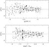 |
Fig. 4 Behavior of the iron abundance as a function of EWR (upper panel) and EWT (lower panel) for a synthetic spectrum computed with vt = 2 km s-1. Filled points show for both cases the shift of a given line owing to the EW error. |
The mean slope, computed by taking into account 200 MonteCarlo simulations of random error distribution, is +0.13 ± 0.02 in the A(Fe)–EWR plane, and –0.01 ± 0.02 in the A(Fe)–EWT plane (always keeping fixed the vt value at the original value of the synthetic spectrum, vt = 2 km s-1). These slopes point out the need to increase vt (of at least 0.2–0.3 km s-1) to erase the residual slope when vt is optimized by using the EWR. On the other hand, adopting the EWT, no relevant change in vt are necessary. This finding exactly reproduces the bias discussed by Magain (1984) (and shown in his Fig. 2), but it seems to contradict to the findings shown in Fig. 3, where the two methods provide lower vt with respect to the true value. Indeed, Magain (1984) demonstrated that vt is systematically overestimated when derived with the classical method.
How can we explain this discrepancy? In the real case (and also in the test performed with synthetic spectra, see Sect. 2), not all lines can be measured and used to infer vt. The effect of the slanting movement of the lines shown in Fig. 4 (upper panel) is critical for very weak lines (where the errors are more relevant), but at low SNR not all these very weak features are detectable, because they are too noisy or indiscernible from the noise envelope. Hence, many weak lines that contribute to the positive slope in the A(Fe)–EWR plane will go out of the detectability threshold, which in turn reduces the positive slope.
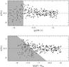 |
Fig. 5 Same of Fig. 4 but highlighting the lines detectable at SNR = 25 (grey points). Grey regions indicate the location of the undetectable lines. |
For a given SNR, a reasonable and generally adopted threshold to measure spectral lines is to assume three times the uncertainty provided by the Cayrel formula. Thus, for SNR = 25 we can measure absorption lines of at least 9 mÅ and 11 mÅ at 5500 and 8000 Å, respectively. Because the difference is negligible along the entire coverage of the spectrum, We conservatively adopted a threshold of 11 mÅ. Figure 5 reports the same results as Fig. 4, but highlighting the lines that are really detectable assuming this threshold (gray points), while the lines located in the gray shaded regions are excluded from the analysis.
The mean slope of the 200 MonteCarlo simulations, computed on the surviving lines, turns out to be of −0.10 ± 0.02 in the A(Fe)–EWR plane, and −0.14 ± 0.02 in the A(Fe)–EWT plane. When we take into account the effective possibility to detect very weak lines with large uncertainties, the situation turns into the opposite of the case described in Fig. 4:
-
the threshold in the A(Fe)–EWT plane turns out to be diagonal, introducing a negative slope and the need to lower vt to erase any trend5;
-
in both cases the derived vt will be lower than the original value of the synthetic spectrum (the same finding discussed above and shown in Fig. 3).
In principle, all these effects are valid for higher SNR as well, but become negligible because the quoted uncertainties in the EW measurement are of only a few percent.
This experiment clarifies the origin of the systematic underestimate of vt with the two approaches (shown in Fig. 3). When vt is derived from EWR, the correlation between the EWR and abundance errors moves the lines in an asymmetric way on the A(Fe)–EWR plane (upper panel of Fig. 4), but the threshold of detectability of the lines will mainly populate the region with A(Fe) > 6.5 dex with respect to other one (as appreciable in the upper panel of Fig. 5), which leads to a negative slope (and an underestimate of vt).
When vt is derived from EWT, the threshold of the line selection shown in the lower panel of Fig. 5 increases the asymmetric distribution of the lines in the plane, always leading to a negative slope (as demonstrated by the average slopes in the two cases) and a slightly lower vt value.
Obviously, the inclusion of weak lines with inaccurate measures will worsen the discrepancy (lower panels in Fig. 3).
To summarize, the vt inferred by using the A(Fe)–EWT plane are not totally free from observational biases. In fact:
-
(a)
the use of A(Fe)–EWT plane partially erases the effect from the correlation between errors in EW and abundances, but also introduces another bias owing to the threshold of detectability of the lines (more relevant and crucial at low SNR), as described above;
-
(b)
errors in A(Fe) and EWT are still not totally independent from each other, because both quantities suffer from uncertainties from the adopted log 10(gf) values. Indeed, an overestimate of the oscillator strength for a given line will provide an overestimate of EWT, but also an underestimate of A(Fe), introducing a negative, spurious slope when EWT is used to infer vt. Note that this effect is secondary, if accurate laboratory oscillator strengths are taken into account. For instance, the typical errors of the Fe I log 10(gf) in the critical compilation by Fuhr & Wiese (2006) are less than 25%. These errors translate into an iron abundance error on the same order of magnitude as on obtained with an error of EW of ~25% or less. The correlation between the errors in log 10(gf) and abundances introduce a spurious slope in the plane A(Fe)-EWT, in a similar way to the spurious slope in the A(Fe)-EWR plane from the correlation between abundance and EWR discussed above. Otherwise, one needs to consider this secondary bias as well only if inaccurate/inhomogeneous atomic data for iron lines are included in the linelist;
-
(c)
if the temperature was inferred by imposing the excitational equilibrium (erasing any slope in A(Fe)–χex plane), θ will also be affected (in a stronger way for low SNR spectra) by the errors in EW, and therefore EWT will also be affected by the same bias, by definition. Note that these last two aspects have not been deeply investigated in the present work.
6. Impact of the number of lines
Previous results are based on a large number of Fe I lines (250), allowing a good sampling of both weak and moderately strong features. This assumption allows avoiding spurious slopes (regardless of the adopted method) caused by inadequate sampling of line strengths.
Some mid/high-resolution multi-object spectrographs offer wavelength coverages that limit the number of available Fe I lines.
A simple test was performed to clarify what difference the number of lines makes. Fifty Fe I lines were randomly extracted from the measured lines in a red giant synthetic spectrum with noise SNR = 25, and vt was redetermined with the two methods. This procedure was repeated by using 200 MonteCarlo extractions. The average values of the vt distributions is very similar to those obtained above, but with a larger dispersion (σ ~ 0.3–0.4 km s-1) with respect to that obtained in the case described in Sect. 4.
If the same check is performed with a synthetic spectrum with SNR=100, the final distributions share dispersions around the mean of about σ ~ 0.15–0.2 km s-1, in both cases, while in the case discussed in Sect. 4 the dispersion was very small (see Fig. 3). These dispersions are also larger than those inferred from EWR and EWT when a large number of transitions is used.
The most discrepant vt values in the derived distributions are obtained when an inadequate sampling of the weak and strong lines is adopted. Indeed, if the experiment is repeated imposing the condition that the 50 random lines are extracted by equally sampling the entire EW range (thus providing a statistically significant sample of weak and strong lines), the dispersion around the mean of the derived distribution of vt is reduced by about a factor of 1.5 and 2 for SNR = 25 and 100 respectively. In this case, the distributions show dispersions around the mean that are barely consistent with those obtained with the entire linelist. We can conclude that the number of used lines and the relative sampling between weak and strong lines are crucial elements that can affect the determination of vt more severely than the choice of the EWR or EWT method in the analysis.
7. Impact of the continuum placement
As already pointed out above, the test performed with synthetic spectra neglects uncertainties arising from the continuum location, because the continuum in artificial spectra is set at unity and totally flat, while in real spectra several additional effects affect its correct identification. In order to clarify how much this source of uncertainty in the EW measurements impacts vt, We performed two simple tests by considering synthetic spectra with SNR = 25:
-
(1)
the EWs were remeasured by adopting a higher and lowercontinuum level with respect to that derived in the previousexperiment. The variations in the continuum level are of ± 5 and ± 10%, translating into a systematic (positive or negative depending by the sign of continuum variation) offset of the derived EWs (the same finding has been discussed in Stetson & Pancino (2008), see their Fig. 2). The differences between vt derived with the EWR and EWT methods are similar to those obtained with the original continuum level;
-
(2)
the synthetic spectra were multiplied with a sinusoidal curve to mimic a fringing-like pattern, similar to that observed in real spectrum. Here likewise there was no relevant difference (within the uncertainties) with the original analysis.
The continuum tracement (for a continuum defined globally along the entire spectrum) does not dramatically affect the results described in Sect. 4 about the relative difference between vt derived with EWR and EWT methods.
8. A real case: UVES spectra of LMC giants
In order to show a case based on real spectra, we derived vt with the two methods for some Large Magellanic Cloud giants stars observed with UVES (Mucciarelli et al. 2009), with typical SNR = 50, which were originally analyzed following the prescriptions by Magain (1984).
Microturbulent velocities computed with the classical method (and fixing the other parameters) are higher by ~0.2–0.25 km s-1 than those obtained with the prescription by Magain (1984); this difference translates into an iron abundance ~0.15 dex lower when the classical approach is adopted.
A point to recall here is that the Teff and vt can be correlated if these quantities are derived with the classical full spectroscopic method. Indeed, the majority of the weak lines have high χex, while several strong transitions have low excitation potentials, which leads to a correlation between χex and the strength of the lines. Also, variations in Teff and vt differently change single and ionized iron lines abundances, which makes it necessary to readjust the surface gravity. The higher vt computed with the classical method implies the need to adjust spectroscopically both Teff and log g, by increasing them and hence reducing the iron abundance difference (by less than 0.1 dex).
To summarize, the absolute difference in iron abundance computed with the two approaches is reduced (by less than 0.1 dex) if a full spectroscopic determination of all atmospherical parameters is performed. Therefore, if one or more parameters are fixed to a certain value, this compensation does not take place and the absolute difference can be higher.
9. Determination of vt: the best strategy
We propose an easy strategy to minimize the effect of the bias discussed above, deriving the vt from EWR, because this is the approach that yields the better results with respect to the true vt of the synthetic spectra used in Sect. 4:
-
(i)
because the determination ofvt is strongly affected by the correlated errors in abundances and EWs, the lines with high uncertainties in the EW measurement need to be discarded. Indeed, as demonstrated in Fig. 3, the inclusion of lines with inaccurate EWs leads to highly incorrect vt with respect to the true value. Basically, the use of lines with EW errors of less than 10% provides a good agreement with the vt value of the synthetic spectra. The reader can use the relations provided in Sect. 4 to estimate the amplitude of the bias in vt as a function of the adopted σEW cutoff. Note that the computation of the EW uncertainty is not provided by all codes developed to measure EWs, but a standard error about the goodness of the fit for each measured line is recommended, through the standard deviation of the local flux residuals after the Gaussian fitting (as performed by DAOSPEC) or by adopting other formulae, i.e. the Cayrel formula or that proposed by Ramirez et al. (2001);
-
(ii)
as shown in Fig. 3, even if an adequate line selection is applied, a residual discrepancy between the derived and true vt of ~0.15 km s-1 remains in the most critical case of SNR = 25. A possible method to reduce this residual discrepancy is to perform a linear fit obtained taking into account the uncertainties in both EWs and abundances (following the approach by Press et al. 1992, as implemented in the FORTRAN routine FITEXY). Errors in EWs were estimated as described in Sect. 4, while the error in the abundance of each individual line was derived by computing the abundance with the EW varied of ± 1σEW. This method to perform the linear fit allows one to obtain values of vt consistent within the errors with the true value of the synthetic spectra (see the first panel of Fig. 3), which reduces the residual discrepancy. Usually in the chemical analysis, the slope in A(Fe) – EWR plane is computed neglecting the uncertainties in the two variables (because this procedure needs the computation of the error in both EW and abundance for each measured line), but this approach (or other approaches to find the linear relation in data with uncertainties in both directions, see e.g. Hogg et al. 2010) is recommended.
10. Conclusions
We draw the following conclusions from the above test:
-
(1)
The method to infer the microturbulent velocity from the EWTprovides the same results (within the quoted uncertainties) as theclassical method for moderate/high SNR (≥70).
-
(2)
For SNR < 70 both methods underestimate the microturbulent velocity, and when low (25) SNR spectra are analyzed, a better agreement with the true vt of the synthetic spectra is found with the classical method based on EWR.
-
(3)
The discrepancy with the true vt value (regardless of the adopted method) worsens when EWs with high uncertainties (generally, the weakest lines in low SNR spectra) are taken into account. This finding points out the need to estimate the quality of the measured EWs for each individual line (a procedure usually not performed in the chemical analysis), to reduce this systematic underestimate.
-
(4)
These results are valid for both giant and dwarf stars, under the assumptions that the strong lines that deviate significantly from the Gaussian approximation are excluded from the analysis.
-
(5)
The number of used lines and the adequate sampling of weak and strong lines for a small number of available iron lines affects the determination of vt more than the adopted approach to infer this parameter.
-
(6)
The simultaneous spectroscopic optimization of all atmospheric parameters is recommended, to compensate errors in the determinations of the parameters.
Note that this is a simplifying assumption. Indeed, the most adopted method to perform a chemical analysis (the so-called full spectroscopic method) is based on the following requirements: (i) the iron abundance is independent of χex (constraint for Teff); (ii) the same abundance should be derived from single and ionized iron lines (constraint for log g); (iii) the iron abundance is independent of the line strength (constraint for vt); (iv) the model metallicity well reproduces the iron abundance (constraint for [M/H]).
Acknowledgments
We thank the referee Matthias Steffen, whose comments and suggestions have significantly improved the paper. We warmly thank Elena Pancino for her useful suggestions and a careful reading of the manuscript.
References
- Asplund, M., Nordlund, A., Trampedach, R., Allen de Prieto, C., & Stein, R. F. 2000, A&A, 359, 729 [NASA ADS] [Google Scholar]
- Böhm-Vitense, E. 1958, ZA, 46, 108 [Google Scholar]
- Cayrel, R. 1988, in The Impact of very high S/N SPectroscopy on Stellar Physics, ed. G. Cayrel de Strobel, & M. Spite, IAU Symp., 132, 345 [Google Scholar]
- Fuhr, J. R., & Wiese, W. L. 2006, JPCRD, 35, 1669 [NASA ADS] [Google Scholar]
- Gray, D. F. 1981, ApJ, 245, 992 [NASA ADS] [CrossRef] [Google Scholar]
- Gray, D. F. 1992, The Observation and analysis of stellar spectra, Cambridge Astrophys. Ser. [Google Scholar]
- Hogg, D. W., Bovy, J., & Lang, D. 2010 [arXiv:1008.4686] [Google Scholar]
- Magain, P. 1984, A&A, 134, 189 [NASA ADS] [Google Scholar]
- Mucciarelli, A., Origlia, L., Ferraro, F. R., & Pancino, E. 2009, ApJ, 659, L134 [NASA ADS] [CrossRef] [Google Scholar]
- Nordlund, A., Spruit, H. C., Ludwig, H.-G., & Trampedach, R. 1997, A&A, 328, 229 [NASA ADS] [Google Scholar]
- Press, W. H.,Teukolsky, A. A., Vetterling, W. T., & Flannery, B. P., Numerical Recipes, 2nd edn. (Cambridge: Cambridge Univ. Press) [Google Scholar]
- Ramirez, S. V., Cohen, J. G., Buss, J., & Briley, M. M., 2001, AJ, 122, 1429 [NASA ADS] [CrossRef] [Google Scholar]
- Ryan, S., A&A, 331, 1051 [Google Scholar]
- Sbordone, L. 2005, Mem. Soc. Astron. Ital. Suppl., 8, 61 [Google Scholar]
- Sbordone, L., Bonifacio, P., Castelli, F., & Kurucz, R. L. 2004, Mem. Soc. Astron. Ital. Suppl., 5, 93 [Google Scholar]
- Steffen, M., & Holweger, H., 2002, A&A, 387, 258 [NASA ADS] [CrossRef] [EDP Sciences] [Google Scholar]
- Stetson, P. B., & Pancino, E. 2008, PASP, 120, 1332 [Google Scholar]
- Takeda, Y. 1992, A&A, 253, 487 [NASA ADS] [Google Scholar]
All Figures
|
Fig. 1 Behavior of the true equivalent widths measured in the synthetic spectrum (without Poissonian noise) computed with the atmospheric parameters of a giant star, as a function of the quantity log 10(gf) − θχex. |
| In the text | |
|
Fig. 2 Difference between the measured and true EW in a synthetic spectrum with SNR = 25 as a function of the true EW. In the left inset we show the behavior of the error in percentage of the measured EW as a function of the true EW, while in the right inset we show the same behavior as a function of the measured EW. |
| In the text | |
|
Fig. 3 Behavior of the measured microturbulent velocity as a function of SNR, derived with the classical method (empty circles) and the prescription by Magain (1984) (filled circles) for a giant star. Each point is the average value obtained by using 200 synthetic spectra of a given SNR, and the errorbars indicate the dispersion around the mean. Dashed lines indicate the original value of vt of the synthetic spectra. Each panel shows the results obtained by considering different thresholds for the residual errors in the EW measurement. |
| In the text | |
|
Fig. 4 Behavior of the iron abundance as a function of EWR (upper panel) and EWT (lower panel) for a synthetic spectrum computed with vt = 2 km s-1. Filled points show for both cases the shift of a given line owing to the EW error. |
| In the text | |
|
Fig. 5 Same of Fig. 4 but highlighting the lines detectable at SNR = 25 (grey points). Grey regions indicate the location of the undetectable lines. |
| In the text | |
Current usage metrics show cumulative count of Article Views (full-text article views including HTML views, PDF and ePub downloads, according to the available data) and Abstracts Views on Vision4Press platform.
Data correspond to usage on the plateform after 2015. The current usage metrics is available 48-96 hours after online publication and is updated daily on week days.
Initial download of the metrics may take a while.