© ESO, 2011

1. Introduction

Several people (e.g., Charbonnel & Talon 2005, 2007; Charbonnel & Zahn 2007) have discussed the importance of properly quantifying the mixing properties of tracers that behave as passive tracers, such as⁷Li. Thus far, the lack of a reliable expression for the diffusivity of a passive tracer was remedied by the use of heuristic expressions which lack predictive power because they are adjusted to reproduce known data. In lieu of empirical relations, one might think of employing the diffusivities of either heat and/or mean molecular weight μ that were derived in Papers I and II. Such an assumption is, however, questionable, because a tracer such as⁷Li is by definition passive since it does not affect the density of the fluid and in consequence, does not affect the velocity field. On the other hand, both T and μ affect the density and for that reason are called active tracers. There is therefore a need to a) construct a diffusivity for passive tracers; b) show how it relates to that of heat and molecular weight; and c) assess its validity before it is used. This is the task of this work.

While the RSM (Reynolds stress model) discussed in I and II provides a methodology to treat the first two items, provided care is taken to account for all the variables in the problem, item c) is more difficult since we are not aware of any direct measurement of a passive tracer diffusivity in astrophysical settings. Since we believe that an assessment is necessary and perhaps even indispensable for the credibility of the model, we show how our results compare with the only case we know of direct measurement of a passive tracer diffusivity. It is not an astrophysical setting but an oceanographic one, the so-called North Atlantic Tracer Release Experiment (NATRE, Ledwell et al. 1993, 1998) in which the tracer SF₆ was released in the ocean. From the measurements in time of its dispersion, a value of the corresponding diffusivity was derived. We applied our model to NATRE and showed that the model predictions fare well with the measured data.

Some of the results that have emerged from this analysis can be summarized as follows:

a) the model is algebraic; b) in the general 3D case, the passive tracer diffusivity is a tensor that depends on stable, unstable stratification, shear (differential rotation), and double diffusion processes; c) in the 1D version of the model, in doubly stable regimes, ∇_μ > 0,   ∇ − ∇_ad < 0, the passive tracer diffusivity is nearly the same as those of the T-μ fields; d) in semi-convection regimes, ∇_μ > 0,   ∇ − ∇_ad > 0, the passive tracer diffusivity is larger than that of the μ-field; and e) in salt fingers regimes,∇_μ < 0,∇ − ∇_ad < 0, the passive scalar diffusivity is smaller than that of the μ-field.

2. Passive tracer flux

Calling c the passive tracer field, we begin with the general conservation equation (d/dt = ∂_t + u_i∂_i), $\frac{\mathrm{d}\mathit{\rho c}}{\mathrm{d}\mathit{t}}\mathrm{=}\frac{\mathit{\partial \rho }{\mathit{J}}_{\mathit{i}}}{\mathit{\partial }{\mathit{x}}_{\mathit{i}}}\mathit{,}$(1a)where u_i is the total velocity field and the diffusion flux J_i is given by Chapman & Cowling (1970): ${\mathit{J}}_{\mathit{i}}\mathrm{=}{\mathit{\chi }}_{\mathit{c}}\mathrm{(}{\mathit{c}}_{\mathit{,i}}\mathrm{+}{\mathit{\kappa }}_{\mathit{T}}{\mathit{T}}^{-1}{\mathit{T}}_{\mathit{,i}}\mathrm{+}{\mathit{\kappa }}_{\mathit{p}}{\mathit{p}}^{-1}{\mathit{p}}_{\mathit{,i}}\mathrm{)}$(1b)with a_,i = ∂a / ∂x_i and where κ_T,κ_p are dimensionless functions. Often, in the literature, J_i includes the density and has the opposite sign and χ_c is called D. We also note that different authors have used different notations, e.g., Eq. (2.1) of Aller & Chapman (1960), Eq. (3) of Schatzman (1969), Eq. (1) of Michaud (1970), and Eq. (1) of Vauclair & Vauclair (1982).

• a)

  mean c-field. In carrying out the mass averaging process (Favre 1969; Canuto 1997, 1999) defined $\overline{\mathit{\rho c}}\mathrm{=}\overline{\mathit{\rho }}\hspace{0.17em}\mathit{C,} \overline{\mathit{\rho c}{\mathit{u}}_{\mathit{i}}}\mathrm{=}\overline{\mathit{\rho }\hspace{0.17em}}\mathit{C}{\mathit{U}}_{\mathit{i}}\mathrm{+}\overline{\mathit{\rho }{\mathit{u}}_{\mathit{i}}^{\mathrm{\prime }}{\mathit{c}}^{\mathrm{\prime }}}\mathit{,}$(2a)we obtain (D_t = ∂_t + U_i∂_i) $\overline{\mathit{\rho }}\frac{\mathrm{D}\mathit{C}}{\mathrm{D}\mathit{t}}\mathrm{=}\mathrm{-}\frac{\mathit{\partial }}{\mathit{\partial }{\mathit{x}}_{\mathit{i}}}\left(\overline{\mathit{\rho }}{\mathit{J}}_{\mathit{i}}^{\mathit{c}}\right)\mathrm{+}\frac{\mathit{\partial }}{\mathit{\partial }{\mathit{x}}_{\mathit{i}}}\left(\overline{\mathit{\rho }}{\mathit{\chi }}_{\mathit{c}}\frac{\mathit{\partial C}}{\mathit{\partial }{\mathit{x}}_{\mathit{i}}}\right)\mathit{,}$(2b)where U_i,C are the mean velocity and mean concentration fields, and the first term on the rhs of (2b) is the turbulent c- flux defined as (primes indicate turbulent variables): $\mathrm{c}\mathrm{-}\mathrm{flux:}\overline{\mathit{\rho }}{\mathit{J}}_{\mathit{i}}^{\mathit{c}}\mathrm{=}\overline{\mathit{\rho }{\mathit{u}}_{\mathit{i}}^{\mathrm{\prime }}{\mathit{c}}^{\mathrm{\prime }}}\mathit{.}$(2c)At first sight, it may look as though Eq. (2b) is unrelated to the T-μ fields or for that matter, to shear and vorticity but, as we show below, the turbulent c-flux (2c) entails all those dependences.

• b)

  passive tracer fluxes. Multiplying (1a) by u_i, Eq. (6a) of Paper I by c and adding the two, we obtain ${\mathit{\partial }}_{\mathit{t}}\mathrm{\left(}\mathit{\rho c}{\mathit{u}}_{\mathit{i}}\mathrm{\right)}\mathrm{+}{\mathit{\partial }}_{\mathit{j}}\mathrm{\left(}\mathit{\rho c}{\mathit{u}}_{\mathit{i}}{\mathit{u}}_{\mathit{j}}\mathrm{\right)}\mathrm{=}\mathit{c}{\mathit{F}}_{\mathit{i}}\mathit{,}$(3a)where F_i was defined in Eq. (6a) of Paper I as ${\mathit{F}}_{\mathit{i}}\mathrm{=}\mathrm{-}{\mathit{p}}_{\mathit{,i}}\mathrm{-}\mathit{\rho }{\mathit{g}}_{\mathit{i}}\mathrm{+}{\mathit{\sigma }}_{\mathit{ij,j}}$(3b)where the last term on the rhs of (3b) is the kinematic viscosity tensor and the other symbols have their usual meaning. Next, we mass average (3a) with the following results $\begin{array}{ccc}\overline{\mathit{\rho c}{\mathit{u}}_{\mathit{i}}}& \mathrm{=}& \overline{\mathit{\rho }}{\mathit{U}}_{\mathit{i}}\mathit{C}\mathrm{+}\overline{\mathit{\rho }{\mathit{u}}_{\mathit{i}}^{\mathrm{\prime }}{\mathit{c}}^{\mathrm{\prime }}}\mathrm{=}\overline{\mathit{\rho }}{\mathit{U}}_{\mathit{i}}\mathit{C}\mathrm{+}\overline{\mathit{\rho }}{\mathit{J}}_{\mathit{i}}^{\mathit{c}}\\ \overline{\mathit{\rho c}{\mathit{u}}_{\mathit{i}}{\mathit{u}}_{\mathit{j}}}& \mathrm{=}& \overline{\mathit{\rho }}{\mathit{U}}_{\mathit{i}}{\mathit{U}}_{\mathit{j}}\mathit{C}\mathrm{+}{\mathit{U}}_{\mathit{k}}\mathrm{(}{\mathit{\delta }}_{\mathit{ik}}{\mathit{J}}_{\mathit{j}}^{\mathit{c}}\mathrm{+}{\mathit{\delta }}_{\mathit{jk}}{{\mathit{J}}_{\mathit{i}}^{\mathit{c}}}^{\mathrm{)}}\mathrm{+}\overline{\mathit{\rho }}{\mathit{R}}_{\mathit{ij}}\mathrm{+}\overline{\mathit{\rho }{\mathit{u}}_{\mathit{i}}^{\mathrm{\prime }}{\mathit{u}}_{\mathit{j}}^{\mathrm{\prime }}{\mathit{c}}^{\mathrm{\prime }}}\end{array}$(3c)where $\overline{\mathit{\rho }}{\mathit{R}}_{\mathit{ij}}\mathrm{=}\overline{\mathit{\rho }{\mathit{u}}_{\mathit{i}}^{\mathrm{\prime }}{\mathit{u}}_{\mathit{j}}^{\mathrm{\prime }}}$ are the Reynolds stresses. Subtracting its mass-averaged from the original equation, we obtain, after several steps, the equation governing the concentration flux: 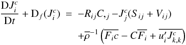$\begin{array}{ccc}\frac{\mathrm{D}{\mathit{J}}_{\mathit{i}}^{\mathit{c}}}{\mathrm{D}\mathit{t}}\mathrm{+}{\mathrm{D}}_{\mathit{f}}\mathrm{\left(}{\mathit{J}}_{\mathit{i}}^{\mathit{c}}\mathrm{\right)}& \mathrm{=}& \mathrm{-}{\mathit{R}}_{\mathit{ij}}\mathit{C}{\mathit{,}}_{\mathit{j}}\mathrm{-}{\mathit{J}}_{\mathit{j}}^{\mathit{c}}\mathrm{(}{\mathit{S}}_{\mathit{ij}}\mathrm{+}{\mathit{V}}_{\mathit{ij}}\mathrm{)}\\ & & \mathrm{+}{\overline{\mathit{\rho }}}^{-1}\mathrm{(}\overline{{\mathit{F}}_{\mathit{i}}\mathit{c}}\mathrm{-}\mathit{C}\overline{{\mathit{F}}_{\mathit{i}}}\mathrm{+}{\overline{{\mathit{u}}_{\mathit{i}}^{\mathrm{\prime }}{\mathit{J}}_{\mathit{k,k}}^{\mathit{c}}}}^{\mathrm{)}}\end{array}$(4a)where 2S_ij = U_i,j + U_j,i,2V_ij = U_i,j − U_j,i, are the shear and vorticity characterizing the mean velocity field. After some further algebraic steps regarding the last terms on the rhs of (4a), we obtain 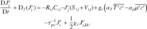$\begin{array}{ccc}\frac{\mathrm{D}{\mathit{J}}_{\mathit{i}}^{\mathit{c}}}{\mathrm{D}\mathit{t}}\mathrm{+}{\mathrm{D}}_{\mathit{f}}\mathrm{\left(}{\mathit{J}}_{\mathit{i}}^{\mathit{c}}\mathrm{\right)}& \mathrm{=}& \mathrm{-}{\mathit{R}}_{\mathit{ij}}\mathit{C}{\mathit{,}}_{\mathit{j}}\mathrm{-}{\mathit{J}}_{\mathit{j}}^{\mathit{c}}\mathrm{(}{\mathit{S}}_{\mathit{ij}}\mathrm{+}{\mathit{V}}_{\mathit{ij}}\mathrm{)}\mathrm{+}{\mathit{g}}_{\mathit{i}}\mathrm{(}{\mathit{\alpha }}_{\mathit{T}}\overline{{\mathit{T}}^{\mathrm{\prime }}{\mathit{c}}^{\mathrm{\prime }}}\mathrm{-}{\mathit{\alpha }}_{\mathit{\mu }}{\overline{{\mathit{\mu }}^{\mathrm{\prime }}{\mathit{c}}^{\mathrm{\prime }}}}^{\mathrm{)}}\\ & & \mathrm{-}{\mathit{\tau }}_{\mathit{pc}}^{-1}{\mathit{J}}_{\mathit{i}}^{\mathit{c}}\mathrm{+}\frac{\mathrm{1}}{\mathrm{2}}{\mathit{\chi }}_{\mathit{c}}{\mathit{J}}_{\mathit{i,kk}}^{\mathit{c}}\mathit{.}\end{array}$(4b)It is interesting to compare (4b) with the corresponding equations for the T-μ fluxes, Eqs. (9e,11b) of Paper I. The first two terms in each of these three equations are similar since they represent the sources of the fluxes given by the interaction of the Reynolds stresses R_ij with the gradients of the corresponding mean variables. The second terms in each of the three equations are also similar since they represent the interaction of the mean shear and vorticity with the fluxes under consideration. The third terms in each expression is where the differences occur. The T-μ fields have similar terms but with opposite signs since the T-μ fields contribute in opposite ways to the density, as Eq. (1b) of Paper I shows. Since the T-μ fields are active tracers, the square terms represent potential energies of the two fields while such a term does not exist in the case of a passive scalar, where we instead have a term that comes from the term g_iρ in the momentum equation, see the second term in (3b); specifically, when we multiply g_iρ by c′, we obtain the term $\overline{{\mathit{\rho }}^{\mathrm{\prime }}{\mathit{c}}^{\mathrm{\prime }}}\mathrm{\to }{\mathit{\alpha }}_{\mathit{T}}\overline{{\mathit{T}}^{\mathrm{\prime }}{\mathit{c}}^{\mathrm{\prime }}}\mathrm{-}{\mathit{\alpha }}_{\mathit{\mu }}\overline{{\mathit{\mu }}^{\mathrm{\prime }}{\mathit{c}}^{\mathrm{\prime }}}$(4c)where we have used Eq. (1b) of Paper I. Finally, since a passive tracer is characterized by a kinematic diffusivity χ_c, the latter gives rise to the last term in (4b). Thus, Eq. (4b) tells us that the c-field interacts not only with the large-scale fields C,U_i, but also with the fluctuating parts of the T-μ fields, as Eq. (4c) clearly shows. To proceed, we need to determine the two fluxes entering the third term in (4b). In the local limit, the first one was given in Eq. (124) of C99, and reads as: $\overline{{\mathit{T}}^{\mathrm{\prime }}{\mathit{c}}^{\mathrm{\prime }}}\mathrm{=}{\mathit{\tau }}_{\mathit{c\theta }}\mathrm{(}{\mathit{\beta }}_{\mathit{i}}{\mathit{J}}_{\mathit{i}}^{\mathit{c}}\mathrm{-}{\mathit{C}}_{\mathit{,i}}{{\mathit{J}}_{\mathit{i}}^{\mathit{h}}}^{\mathrm{)}}\mathit{,} {\mathit{\beta }}_{\mathit{i}}\mathrm{=}\mathrm{-}\hspace{0.17em}\mathit{\partial T}\mathit{/}\mathit{\partial }{\mathit{x}}_{\mathit{i}}\mathrm{-}{\mathit{\lambda }}_{\mathit{i}}\mathit{g}{\mathit{c}}_{\mathit{p}}^{-1}$(4d)where ${\mathit{\lambda }}_{\mathit{i}}\mathrm{=}\mathrm{-}\mathrm{(}\mathit{g}\overline{\mathit{\rho }}{\mathrm{)}}^{-1}\mathit{\partial }\overline{\mathit{p}}\mathit{/}\mathit{\partial }{\mathit{x}}_{\mathit{i}}$. 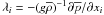Analogously, we derive $\overline{{\mathit{\mu }}^{\mathrm{\prime }}{\mathit{c}}^{\mathrm{\prime }}}\mathrm{=}\mathrm{-}{\mathit{\tau }}_{\mathit{c\mu }}\mathrm{(}{\mathit{J}}_{\mathit{i}}^{\mathit{c}}{\overline{\mathit{\mu }}}_{\mathit{,i}}\mathrm{+}{\mathit{C}}_{\mathit{,i}}{{\mathit{J}}_{\mathit{i}}^{\mathit{\mu }}}^{\mathrm{)}}\mathit{.}$(4e)Substituting these two relations into (4b) and taking the stationary limit, we obtain that the passive tracer flux is given by the following equation: $\mathrm{(}{\mathit{\delta }}_{\mathit{ij}}\mathrm{+}{\mathit{\omega }}_{\mathit{ij}}\mathrm{)}{\mathit{J}}_{\mathit{j}}^{\mathit{c}}\mathrm{=}\mathrm{-}{\mathit{e}}_{\mathit{ij}}{\mathit{C}}_{\mathit{,j}}$(5a)where $\begin{array}{c}\\ {\mathit{e}}_{\mathit{ij}}\mathrm{=}{\mathit{\tau }}_{\mathrm{pc}}\left[{\mathit{R}}_{\mathit{ij}}\mathrm{+}{\mathit{g}}_{\mathit{i}}\left({\mathit{\alpha }}_{\mathit{T}}{\mathit{\tau }}_{\mathit{c\theta }}{\mathit{J}}_{\mathit{j}}^{\mathit{h}}\mathrm{-}{\mathit{\alpha }}_{\mathit{\mu }}{\mathit{\tau }}_{\mathit{c\mu }}{\mathit{J}}_{\mathit{j}}^{\mathit{\mu }}\right)\right]\\ {\mathit{\omega }}_{\mathit{ij}}\mathrm{=}\hspace{0.17em}{\mathit{\tau }}_{\mathrm{pc}}\mathrm{[}{\mathit{S}}_{\mathit{ij}}\mathrm{+}{\mathit{V}}_{\mathit{ij}}\mathrm{-}{\mathit{g}}_{\mathit{i}}{\mathrm{(}{\mathit{\alpha }}_{\mathit{T}}{\mathit{\tau }}_{\mathit{c\theta }}{\mathit{\beta }}_{\mathit{j}}\mathrm{+}{\mathit{\alpha }}_{\mathit{\mu }}{\mathit{\tau }}_{\mathit{c\mu }}{\overline{\mathit{\mu }}}_{\mathit{,j}}\mathrm{)}}^{\mathrm{]}}\mathit{.}\end{array}$(5b)As for the dissipation-relaxation time scales ${\mathit{\tau }}_{\mathrm{pc}}\mathit{,}{\mathit{\tau }}_{\mathit{c\theta }}\mathit{,}{\mathit{\tau }}_{\mathit{c\mu }}$(5c)we introduce the following notation and approximation: ${\mathit{\alpha }}_{\mathrm{1}}\mathrm{=}\frac{{\mathit{\tau }}_{\mathrm{pc}}}{\mathit{\tau }}\mathit{,} {\mathit{\alpha }}_{\mathrm{2}}\mathrm{=}\frac{{\mathit{\tau }}_{\mathit{c\theta }}}{\mathit{\tau }}\mathrm{=}\frac{{\mathit{\tau }}_{\mathit{c\mu }}}{\mathit{\tau }}$(5d)where τ = 2K / ε is the eddy turnover time scale and K-ε are the eddy kinetic energy and its rate of dissipation. The second relation in (5d) rests on the assumption that a passive tracer has the same dissipation time scale as the active tracers T and μ. Equations (5b) then become $\begin{array}{ccc}{\mathit{e}}_{\mathit{ij}}& \mathrm{=}& {\mathit{\alpha }}_{\mathrm{1}}\mathit{\tau }\left[{\mathit{R}}_{\mathit{ij}}\mathrm{+}{\mathit{g}}_{\mathit{i}}\mathit{\tau }{\mathit{\alpha }}_{\mathrm{2}}\left({\mathit{\alpha }}_{\mathit{T}}{\mathit{J}}_{\mathit{j}}^{\mathit{h}}\mathrm{-}{\mathit{\alpha }}_{\mathit{\mu }}{\mathit{J}}_{\mathit{j}}^{\mathit{\mu }}\right)\right]\\ {\mathit{\omega }}_{\mathit{ij}}& \mathrm{=}& {\mathit{\alpha }}_{\mathrm{1}}\mathit{\tau }\mathrm{[}{\mathit{S}}_{\mathit{ij}}\mathrm{+}{\mathit{V}}_{\mathit{ij}}\mathrm{-}{\mathit{g}}_{\mathit{i}}\mathit{\tau }{\mathit{\alpha }}_{\mathrm{2}}{\mathrm{(}{\mathit{\alpha }}_{\mathit{T}}{\mathit{\beta }}_{\mathit{j}}\mathrm{+}{\mathit{\alpha }}_{\mathit{\mu }}{\overline{\mathit{\mu }}}_{\mathit{,j}}\mathrm{)}}^{\mathrm{]}}\mathit{.}\end{array}$(5e)The derivation of the equation for the c-flux is now complete except for the two dimensionless variables α_1,2 which we discuss in the next section. We note the following points. First, the passive tracer flux depends on shear, vorticity, T and μ-gradients. Second, using the Hamilton-Cayley theorem, one can rewrite (5a) in the following form: ${\mathit{J}}_{\mathit{i}}^{\mathit{c}}\mathrm{=}\mathrm{-}\mathrm{(}{\mathit{K}}_{\mathit{c}}{\mathrm{)}}_{\mathit{ij}}\frac{\mathit{\partial C}}{\mathit{\partial }{\mathit{x}}_{\mathit{j}}}$(5f)where the tensor diffusivity tensor (K_c)_ij can be written down explicitly (see C99). Third, as for the functions α_1,2, relations (13i) of Paper I show that the forms of π_1,4 defined in Eq. (10c) of Paper I conserve the T-μ symmetry. It is therefore tempting to identify α₁ with either π_1,4 because they are both potentially acceptable candidates. However, since we have no reason to chose one over the other, the construction of the function, ${\mathit{\alpha }}_{\mathrm{1}\mathit{,}\mathrm{2}}\mathrm{=}\mathit{f}\mathrm{\left(}{\mathit{\pi }}^{\mathrm{\prime }}\mathit{s}\mathrm{\right)}\mathit{,}$(5g)is a non trivial problem that we discuss in the next section.

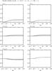Fig. 1 Doubly Stable case, ∇μ > 0,   ∇ − ∇ad < 0, Rμ < 0. The dimensionless mixing efficiencies, defined in Eq. (6d), for the case of a passive tracer, spice, and the ratios of the former with those of μ, heat, buoyancy, and spice.

3. The functions α_1,2

To determine the functions α_1,2, we suggest the following procedure. Let us consider the 1D version of Eqs. (5). Using the notation ${\mathit{J}}_{\mathrm{3}}^{\mathit{c}}\mathrm{\equiv }{\mathit{J}}_{\mathit{c}}$, we derive that ${\mathit{J}}_{\mathit{c}}\mathrm{=}\mathrm{-}\frac{{\mathit{e}}_{\mathrm{33}}}{\mathrm{1}\mathrm{+}{\mathit{\omega }}_{\mathrm{33}}}\frac{\mathit{\partial C}}{\mathit{\partial z}}\mathrm{\equiv }\mathrm{-}{\mathit{K}}_{\mathit{c}}\frac{\mathit{\partial C}}{\mathit{\partial z}}\mathrm{·}$(6a)Using the relation in (Paper II, footnote 1), it is easy to show that ${\mathit{\omega }}_{\mathrm{33}}\mathrm{=}{\mathit{\alpha }}_{\mathrm{1}}{\mathit{\alpha }}_{\mathrm{2}}\mathrm{(}\mathit{\tau N}{\mathrm{)}}^{\mathrm{2}}\mathit{,} {\mathit{N}}^{\mathrm{2}}\mathrm{=}\mathrm{-}\mathit{g}{\mathit{\rho }}_{\mathrm{0}}^{-1}\mathit{\partial }\overline{\mathit{\rho }}\mathit{/}\mathit{\partial z}\mathit{.}$(6b)The computation of e₃₃ is a bit more involved but using relations (Paper II, footnote 1) and (Paper I, Appendix C), we obtain the following result ${\mathit{e}}_{\mathrm{33}}\mathrm{=}{\mathit{\alpha }}_{\mathrm{1}}\mathit{\tau }\overline{{\mathit{w}}^{\mathrm{2}}}\mathrm{[}\mathrm{1}\mathrm{-}{\mathit{\alpha }}_{\mathrm{2}}\mathrm{(}\mathit{\tau N}{\mathrm{)}}^{\mathrm{2}}{\mathit{A}}_{\mathit{\rho }}\mathrm{]}\mathit{,} {\mathit{A}}_{\mathit{\rho }}\mathrm{=}\mathrm{(}{\mathit{A}}_{\mathit{h}}\mathrm{-}{\mathit{R}}_{\mathit{\mu }}{\mathit{A}}_{\mathit{\mu }}\mathrm{)}\mathrm{(}\mathrm{1}\mathrm{-}{\mathit{R}}_{\mathit{\mu }}{\mathrm{)}}^{-1}$(6c)where R_μ = ∇_μ(∇ − ∇_ad)^-1 is the so-called density ratio and the functions A_h,μ are given in (Paper I, Appendix C). Since the form of K_c is also of the type (Paper II, Eqs. 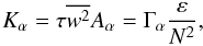(6b, c)), namely (α = h,μ,c), ${\mathit{K}}_{\mathit{\alpha }}\mathrm{=}\mathit{\tau }\overline{{\mathit{w}}^{\mathrm{2}}}{\mathit{A}}_{\mathit{\alpha }}\mathrm{=}{\mathrm{\Gamma }}_{\mathit{\alpha }}\frac{\mathit{\epsilon }}{{\mathit{N}}^{\mathrm{2}}}\mathit{,}$(6d)the corresponding A_c is given by ${\mathit{A}}_{\mathit{c}}\mathrm{=}\frac{{\mathit{\alpha }}_{\mathrm{1}}}{\mathrm{1}\mathrm{+}{\mathit{\alpha }}_{\mathrm{1}}{\mathit{\alpha }}_{\mathrm{2}}\mathrm{(}\mathit{\tau N}{\mathrm{)}}^{\mathrm{2}}}\mathrm{[}\mathrm{1}\mathrm{-}{\mathit{\alpha }}_{\mathrm{2}}\mathrm{(}\mathit{\tau N}{\mathrm{)}}^{\mathrm{2}}{\mathit{A}}_{\mathit{\rho }}\mathrm{]}\mathit{.}$(6e)The dimensionless functions Γ in (6d) are known as mixing efficiencies, and they were discussed in Paper II, Sect. 3. To double check (6e), in Appendix A we re-derive it using a 1D model from the very beginning. If we compare the forms of the functions A_h,μ with that of A_c, we notice that they are different, which is why we stated earlier that the identification of K_c with either K_h and/or K_μ is hard to justify. The point will be clearer when we plot such diffusivities and their ratios in Figs. 1–3.

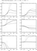Fig. 2 Same as in Fig. 1 but for the case of semi-convection ∇μ > 0,   ∇ − ∇ad > 0, Rμ > 1. The values of Rμ are the reciprocal of those of the case in Fig. 3.

Fig. 3 Same as in Fig. 1 but for the case of salt-fingers, ∇μ < 0,∇ − ∇ad < 0, Rμ < 1.

Next, we consider the active tracer represented by the μ-field and take the limit in which the α_μcontraction coefficient becomes vanishingly small ${\mathit{\alpha }}_{\mathit{\mu }}\mathrm{~}\mathrm{(}\mathit{\partial \rho }\mathit{/}\mathit{\partial \mu }{\mathrm{)}}_{\mathit{T}}\mathrm{\to }\mathrm{0}\mathit{,} {\mathit{R}}_{\mathit{\mu }}\mathrm{\to }\mathrm{0.}$(7a)Physically, (7a) implies that a change in μ does not affect the density, in which case the μ-field behaves like a passive tracer. In this limit, we should therefore have: ${\mathit{\alpha }}_{\mathit{\mu }}\mathrm{\to }\mathrm{0}\mathit{,} {\mathit{R}}_{\mathit{\mu }}\mathrm{\to }\mathrm{0}\mathrm{:} {\mathit{K}}_{\mathit{c}}\mathrm{\to }{\mathit{K}}_{\mathit{\mu }}\mathit{,} {\mathit{A}}_{\mathit{c}}\mathrm{\to }{\mathit{A}}_{\mathit{\mu }}$(7b)Since K_c depends on the functions α_1,2 and K_μ depends on the π′s, the limit (7b) will allow us to establish a relation between the α_1,2 and the π′s for which we have an explicit form (Paper I, Eq. (13i)). We begin with Eq. (6e), which now becomes ${\mathit{R}}_{\mathit{\mu }}\mathrm{\to }\mathrm{0}\mathrm{:} {\mathit{A}}_{\mathit{c}}\mathrm{\to }\frac{{\mathit{\alpha }}_{\mathrm{1}}}{\mathrm{1}\mathrm{+}{\mathit{\alpha }}_{\mathrm{1}}{\mathit{\alpha }}_{\mathrm{2}}\mathrm{(}\mathit{\tau N}{\mathrm{)}}^{\mathrm{2}}}\mathrm{[}\mathrm{1}\mathrm{-}{\mathit{\alpha }}_{\mathrm{2}}\mathrm{(}\mathit{\tau N}{\mathrm{)}}^{\mathrm{2}}{\mathit{A}}_{\mathit{h}}\mathrm{]}$(8a)where A_h is given in Appendix C of Paper I which, in this limit, reads as follows: $\begin{array}{ccc}\mathit{D}{\mathit{A}}_{\mathit{h}}& \mathrm{\to }& {\mathit{\pi }}_{\mathrm{4}}\mathrm{(}\mathrm{1}\mathrm{+}\mathit{\eta x}\mathrm{)}\mathit{,} \mathit{D}\mathrm{=}\mathrm{(}\mathrm{1}\mathrm{+}\mathit{\eta x}\mathrm{)}\mathrm{(}\mathrm{1}\mathrm{+}\mathit{\mu x}\mathrm{)}\mathit{,}\\ \mathit{\eta }& \mathrm{\to }& {\mathit{\pi }}_{\mathrm{1}}{\mathit{\pi }}_{\mathrm{2}}\mathit{,} \mathit{\mu }\mathrm{\to }{\mathit{\pi }}_{\mathrm{1}}{\mathit{\pi }}_{\mathrm{3}}\mathit{.}\end{array}$(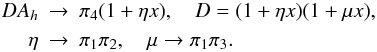8b)We next consider the form of A_μ given in Appendix C of Paper I, $\mathit{D}{\mathit{A}}_{\mathit{\mu }}\mathrm{=}{\mathit{\pi }}_{\mathrm{1}}\mathrm{(}\mathrm{1}\mathrm{+}\mathit{\mu x}\mathrm{-}{\mathit{\pi }}_{\mathrm{2}}{\mathit{\pi }}_{\mathrm{4}}\mathit{x}\mathrm{)}\mathit{.}$(8c)It is easy to verify that the third relation (7b) is satisfied if we take ${\mathit{R}}_{\mathit{\mu }}\mathrm{=}\mathrm{0}\mathrm{:} {\mathit{\alpha }}_{\mathrm{1}}\mathrm{=}{\mathit{\pi }}_{\mathrm{1}}\mathit{,}{\mathit{\alpha }}_{\mathrm{2}}\mathrm{=}{\mathit{\pi }}_{\mathrm{2}}\mathit{.}$(8d)By repeating the same procedure with the T-field instead, we obtain ${\mathit{R}}_{\mathit{\mu }}\mathrm{=}\mathrm{\infty :} {\mathit{\alpha }}_{\mathrm{1}}\mathrm{=}{\mathit{\pi }}_{\mathrm{4}}\mathrm{=}{\mathit{\pi }}_{\mathrm{1}}\mathit{,}{\mathit{\alpha }}_{\mathrm{2}}\mathrm{=}{\mathit{\pi }}_{\mathrm{2}}\mathit{,}$(8e)which is identical to (8d), thus assuring the validity of the procedure. Next, since the shortest time scale dominates, we begin by writing 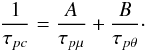$\frac{\mathrm{1}}{{\mathit{\tau }}_{\mathit{pc}}}\mathrm{=}\frac{\mathit{A}}{{\mathit{\tau }}_{\mathit{p\mu }}}\mathrm{+}\frac{\mathit{B}}{{\mathit{\tau }}_{\mathit{p\theta }}}\mathrm{·}$(9)Introducing the π′s from their definition (10c) of Paper I and α₁ from (5d), we choose A,B in (9) to satisfy the two requirements (8d,e). The result is ${\mathit{\alpha }}_{\mathrm{1}}\mathrm{=} \frac{{\mathit{R}}_{\mathit{\mu }}\mathrm{+}{\mathit{R}}_{\mathit{\mu }}^{-1}}{{\mathit{R}}_{\mathit{\mu }}{\mathit{\pi }}_{\mathrm{4}}^{-1}\mathrm{+}{\mathit{R}}_{\mathit{\mu }}^{-1}{\mathit{\pi }}_{\mathrm{1}}^{-1}}\mathrm{·}$(10)Admittedly, relation (10) is not the only possible functional dependence that satisfies the limits (8d,e), but we have chosen it for its simplicity. As for α₂, its identification with π₂ seems unproblematic: ${\mathit{\alpha }}_{\mathrm{2}}\mathrm{=}{\mathit{\pi }}_{\mathrm{2}}\mathit{.}$(11)

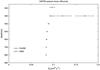Fig. 4 The z-profile of the predicted passive tracer diffusivity vs. the values measured at NATRE.

4. Results

Using the previous results and the variables (τN)² from solving Eqs. (9c-e) of Paper II, Figs. 1–3 show results for different values of Ri and R_μ. In Fig. 1, corresponding to the Doubly-Stable case ∇_μ > 0,   ∇ − ∇_ad < 0 and thus R_μ < 0, we present the dimensionless mixing efficiencies Γ; see Eq. (6d), for a passive tracer panel a) and in panel b) we present the case of spice (a term borrowed from oceanography) defined as σ ≡ α_TT + α_μμ. Since σ is invariant under the exchange of the T and μ fields, it could be viewed as a possible candidate for a passive tracer. The corresponding mixing efficiency is ${\mathrm{\Gamma }}_{\mathit{\sigma }}\mathrm{=}\mathrm{(}{\mathrm{\Gamma }}_{\mathit{h}}\mathrm{+}{\mathit{R}}_{\mathit{\mu }}{\mathrm{\Gamma }}_{\mathit{\mu }}\mathrm{)}\mathrm{(}\mathrm{1}\mathrm{+}{\mathit{R}}_{\mathit{\mu }}{\mathrm{)}}^{-1}$(12)In the remaining panels c)–f) we exhibit the ratios of the mixing efficiencies of a passive tracer with those of μ, heat, buoyancy and spice. As one can observe from panels c)–f), for all practical purposes, there is little difference between the diffusivity of a passive tracer and that of μ, heat or spice. However, since a doubly-stable situation is uncommon, the case is rather academic. In Fig. 2 we present the results for the case of semi-convection, ∇_μ > 0,   ∇ − ∇_ad > 0, and thus R_μ > 1. As one can observe from panel c), the passive tracer diffusivity is larger than that of μ by up to a factor of two and it is smaller than that of heat by the same amount. Finally, in Fig. 3 we present the results for the case of salt-fingers, ∇_μ < 0,∇ − ∇_ad < 0 and thus R_μ < 1, in which case we notice that the passive tracer mixing efficiency is smaller than that of μ but larger than that of heat by roughly the same amount.

5. Assessment of the model prediction against the NATRE data

As an assessment of the model, we present a comparison of the model results with those of the only case we know in which a passive tracer diffusivity was measured directly. It is not an astrophysical case but an oceanographic one corresponding to the experiment NATRE (North Atlantic Tracer Release Experiment) in which the tracer SF₆ was released in the middle of the Atlantic Ocean at the depth of approximately 400 m. It was monitored for several months, and a diffusivity was deduced from the dispersion in time. For details, the reader should consult the original papers by Ledwell et al. (1993, 1998). In the oceanographic case, the role of the μ field is played by salinity, and R_μ is denoted by R_ρ defined analogously as the ratio of the salinity to the temperature z-gradients. In Fig. 4 we present the z-profile of the measured diffusivity vs. the one predicted by the present model in its 1D version presented in Appendix A. The model’s results were obtained using the z-profile of the density ratio R_ρ from the measurements themselves (Laurent & Schmitt 1999). The functions A_h,μ that enter the second of (6c) were constructed using relations (Paper II, Eq. (6d)) in which the heat-to-salt flux ratio “r” was computed from its definition, Paper II, Eq. (7b). The variable x in A_h,μ was obtained by solving Eqs. (Paper II, Eqs. (9c–e)), and the variable $\overline{{\mathit{w}}^{\mathrm{\prime }\mathrm{2}}}\mathit{/}\mathit{K}$ is given by Eq. (Paper II, Eq. (6h)). The model reproduces the measured data fairly well.

6. Summary and conclusions

As one may have guessed on physical grounds, the diffusivity of a passive tracer is not the same as that of active tracers such as temperature, buoyancy, and mean molecular weight. The derivation presented in this paper makes that clear, and the results shown in Figs. 1–3 quantify that relationship, specifically, the ratios of the diffusivities of passive vs. active tracers. The model results are algebraic, hence not difficult to implement in stellar structure-evolution codes.

References

Appendix A: 1D Passive tracer vertical flux

In order to derive the vertical flux of a passive tracer field denoted by c, we begin with the general equation ${\mathit{\partial }}_{\mathit{t}}\mathit{\rho c}\mathrm{+}{\mathit{\partial }}_{\mathit{i}}\left(\mathit{\rho c}{\mathit{u}}_{\mathit{i}}\right)\mathrm{=}{\mathit{\chi }}_{\mathit{c}}\mathit{\rho }{\mathit{\partial }}_{\mathit{i}}^{\mathrm{2}}\mathit{c,}$(A.1)where the rhs represents molecular effects with a kinematic diffusivity χ_c. We split the c,u_i fields into an average and a fluctuating component, c = C + c′ and ${\mathit{u}}_{\mathit{i}}\mathrm{=}{\mathit{U}}_{\mathit{i}}\mathrm{+}{\mathit{u}}_{\mathit{i}}^{{}^{\mathrm{\prime }}}$ and proceed as follows. After introducing the above relations in (A.1), using the incompressibility condition, averaging the result, and subtracting it from the initial equation for the total c-field, algebraic steps lead to the following equation for the fluctuating component (D_t = ∂_t + U_i∂_i): ${\mathit{D}}_{\mathit{t}}{\mathit{c}}^{\mathrm{\prime }}\mathrm{+}{\mathit{u}}_{\mathit{i}}^{\mathrm{\prime }}{\mathit{\partial }}_{\mathit{i}}\mathit{C}\mathrm{+}{\mathit{\partial }}_{\mathit{i}}\mathrm{(}{\mathit{u}}_{\mathit{i}}^{\mathrm{\prime }}{\mathit{c}}^{\mathrm{\prime }}\mathrm{-}{\overline{{\mathit{u}}_{\mathit{i}}^{\mathrm{\prime }}{\mathit{c}}^{\mathrm{\prime }}}}^{\mathrm{)}}\mathrm{=}{\mathit{\chi }}_{\mathit{c}}{\mathit{\partial }}_{\mathit{i}}^{\mathrm{2}}{\mathit{c}}^{\mathrm{\prime }}\mathit{.}$(A.2)Using an analogous procedure applied to the velocity field described by the Navier-Stokes equations, we derive the equation for the field w′ which reads as ${\mathit{\partial }}_{\mathit{t}}{\mathit{w}}^{\mathrm{\prime }}\mathrm{=}\mathrm{-}{\mathit{\rho }}_{\mathrm{0}}^{-1}{\mathit{\partial }}_{\mathit{z}}{\mathit{p}}^{\mathrm{\prime }}\mathrm{-}\mathit{g}{\mathit{\rho }}_{\mathrm{0}}^{-1}{\mathit{\rho }}^{\mathrm{\prime }}\mathrm{-}{\mathit{\partial }}_{\mathit{j}}\left({\mathit{w}}^{\mathrm{\prime }}{\mathit{u}}_{\mathit{j}}^{\mathrm{\prime }}\mathrm{-}\overline{{\mathit{w}}^{\mathrm{\prime }}{\mathit{u}}_{\mathit{j}}^{\mathrm{\prime }}}\right)\mathrm{+}\mathit{\nu }{\mathit{\partial }}_{\mathit{i}}^{\mathrm{2}}{\mathit{w}}^{\mathrm{\prime }}$(A.3)where ν is the kinematic viscosity. As expected, the averages of either (A.2–A.3) yield 0 = 0 since all fluctuating variables have a zero average. We also recall that ${\mathit{\rho }}^{\mathrm{\prime }}{\mathit{\rho }}_{\mathrm{0}}^{-1}\mathrm{=}\mathrm{-}{\mathit{\alpha }}_{\mathit{T}}{\mathit{T}}^{\mathrm{\prime }}\mathrm{+}{\mathit{\alpha }}_{\mathit{\mu }}{\mathit{\mu }}^{\mathrm{\prime }}$, where T′,   μ′are the fluctuating components of the T and μ fields. The next step consists of multiplying Eq. (A.2) by w′ and Eq. (A.3) by c′, averaging the results, and summing the two equations. The result is the dynamic equation for the vertical flux of the passive tracer ${\mathit{J}}_{\mathit{c}}\mathrm{=}\overline{{\mathit{w}}^{\mathrm{\prime }}{\mathit{c}}^{\mathrm{\prime }}}$: ${\mathit{\partial }}_{\mathit{t}}{\mathit{J}}_{\mathit{c}}\mathrm{=}\mathrm{-}\overline{{\mathit{w}}^{\mathrm{\prime }\mathrm{2}}}{\mathit{\partial }}_{\mathit{z}}\mathit{C}\mathrm{+}\mathit{g}\mathrm{(}{\mathit{\alpha }}_{\mathit{T}}\overline{{\mathit{T}}^{\mathrm{\prime }}{\mathit{c}}^{\mathrm{\prime }}}\mathrm{-}{\mathit{\alpha }}_{\mathit{\mu }}{\overline{{\mathit{\mu }}^{\mathrm{\prime }}{\mathit{c}}^{\mathrm{\prime }}}}^{\mathrm{)}}\mathrm{-}{\mathit{\tau }}_{\mathrm{pc}}^{-1}{\mathit{J}}_{\mathit{c}}$(A.4)where we have lumped the pressure correlation and the dissipation terms together into the dissipation-relaxation time scale τ_pc. Next, we must construct the two correlations $\overline{{\mathit{T}}^{\mathrm{\prime }}{\mathit{c}}^{\mathrm{\prime }}}\mathit{,}\hspace{0.17em}\overline{{\mathit{\mu }}^{\mathrm{\prime }}{\mathit{c}}^{\mathrm{\prime }}}$. This is done by using the two equations for the fluctuating T-μ fields, which are obtained using a procedure analogous to the one used to arrive at (A.2). The results are $\begin{array}{ccc}{\mathit{D}}_{\mathit{t}}{\mathit{T}}^{\mathrm{\prime }}\mathrm{+}{\mathit{u}}_{\mathit{i}}^{\mathrm{\prime }}{\mathit{\partial }}_{\mathit{i}}\overline{\mathit{T}}\mathrm{+}{\mathit{\partial }}_{\mathit{i}}\mathrm{(}{\mathit{u}}_{\mathit{i}}^{\mathrm{\prime }}{\mathit{T}}^{\mathrm{\prime }}\mathrm{-}{\overline{{\mathit{u}}_{\mathit{i}}^{\mathrm{\prime }}{\mathit{T}}^{\mathrm{\prime }}}}^{\mathrm{)}}& \mathrm{=}& {\mathit{\chi }}_{\mathit{\theta }}{\mathit{\partial }}_{\mathit{i}}^{\mathrm{2}}{\mathit{T}}^{\mathrm{\prime }}\mathit{,}\\ {\mathit{D}}_{\mathit{t}}{\mathit{\mu }}^{\mathrm{\prime }}\mathrm{+}{\mathit{u}}_{\mathit{i}}^{\mathrm{\prime }}{\mathit{\partial }}_{\mathit{i}}\overline{\mathit{\mu }}\mathrm{+}{\mathit{\partial }}_{\mathit{i}}\mathrm{(}{\mathit{u}}_{\mathit{i}}^{\mathrm{\prime }}{\mathit{\mu }}^{\mathrm{\prime }}\mathrm{-}{\overline{{\mathit{u}}_{\mathit{i}}^{\mathrm{\prime }}{\mathit{\mu }}^{\mathrm{\prime }}}}^{\mathrm{)}}& \mathrm{=}& {\mathit{\chi }}_{\mathit{\mu }}{\mathit{\partial }}_{\mathit{i}}^{\mathrm{2}}{\mathit{\mu }}^{\mathrm{\prime }}\end{array}$(A.5)where the χ′s represent molecular diffusivities. If we multiply the first of (A.5) by c′ and the second by T′, summing the two relations after averaging them, we obtain the two equations $\begin{array}{ccc}{\mathit{\partial }}_{\mathit{t}}\overline{{\mathit{T}}^{\mathrm{\prime }}{\mathit{c}}^{\mathrm{\prime }}}\mathrm{=}\mathrm{-}\left({\mathit{J}}_{\mathit{h}}{\mathit{C}}_{\mathit{,z}}\mathrm{-}{\mathit{J}}_{\mathit{c}}\mathit{\beta }\right)\mathrm{-}{\mathit{\tau }}_{\mathit{c\theta }}^{-1}\overline{{\mathit{T}}^{\mathrm{\prime }}{\mathit{c}}^{\mathrm{\prime }}}& & \\ {\mathit{\partial }}_{\mathit{t}}\overline{{\mathit{\mu }}^{\mathrm{\prime }}{\mathit{c}}^{\mathrm{\prime }}}\mathrm{=}\mathrm{-}\mathrm{(}{\mathit{J}}_{\mathit{\mu }}{\mathit{C}}_{\mathit{,z}}\mathrm{+}{\mathit{J}}_{\mathit{c}}{\overline{\mathit{\mu }}}_{\mathit{,z}}\mathrm{)}\mathrm{-}{\mathit{\tau }}_{\mathit{cs}}^{-1}\overline{{\mathit{\mu }}^{\mathrm{\prime }}{\mathit{c}}^{\mathrm{\prime }}}& & \end{array}$\newpage \noindentwhere, as in Eq. (A.4), the two time scales τ_cθ and τ_cs represent the relaxation-dissipation times scales of the corresponding correlations. For simplicity, we have neglected the third-order moments. In Eqs. (A.6, A.7), J_h,μ are the vertical fluxes of heat and μ whose form was derived in Eq. (C.1) of Paper I to be ${\mathit{J}}_{\mathit{h}}\mathrm{=}\overline{{\mathit{w}}^{\mathrm{\prime }}{\mathit{T}}^{\mathrm{\prime }}}\mathrm{=}{\mathit{K}}_{\mathit{h}}\mathit{\beta ,} {\mathit{J}}_{\mathit{\mu }}\mathrm{=}\overline{{\mathit{w}}^{\mathrm{\prime }}{\mathit{\mu }}^{\mathrm{\prime }}}\mathrm{=}\mathrm{-}{\mathit{K}}_{\mathit{\mu }}{\overline{\mathit{\mu }}}_{\mathit{,z}}\mathit{,}$(A.8)where K_h,μ are the heat and μ diffusivities whose general form is given by relations (6b,c) of Paper II: ${\mathit{K}}_{\mathit{\alpha }}\mathrm{=}\mathit{\tau }\overline{{\mathit{w}}^{\mathrm{2}}}{\mathit{A}}_{\mathit{\alpha }}\mathrm{=}{\mathrm{\Gamma }}_{\mathit{\alpha }}\frac{\mathit{\epsilon }}{{\mathit{N}}^{\mathrm{2}}}\mathrm{·}$(A.9)The explicit form of $\overline{{\mathit{w}}^{\mathrm{2}}}$, which is not needed in this context, is given by Appendix C of Paper I. Taking the stationary limits in Eqs. (A.4, A.6, A.7) and using (A.8), we obtain the desired form of the vertical flux of a passive tracer ${\mathit{J}}_{\mathit{c}}\mathrm{=}\overline{{\mathit{w}}^{\mathrm{\prime }}{\mathit{c}}^{\mathrm{\prime }}}\mathrm{=}\mathrm{-}{\mathit{K}}_{\mathit{c}}\frac{\mathit{\partial C}}{\mathit{\partial z}}\mathit{,}$(A.10)where the dimensionless function A_c is given by ${\mathit{A}}_{\mathit{c}}\mathrm{=}\frac{{\mathit{\alpha }}_{\mathrm{1}}}{\mathrm{1}\mathrm{+}{\mathit{\alpha }}_{\mathrm{1}}{\mathit{\alpha }}_{\mathrm{2}}\mathrm{(}\mathit{\tau N}{\mathrm{)}}^{\mathrm{2}}}\mathrm{[}\mathrm{1}\mathrm{-}{\mathit{\alpha }}_{\mathrm{2}}\mathrm{(}\mathit{\tau N}{\mathrm{)}}^{\mathrm{2}}{\mathit{A}}_{\mathit{\rho }}\mathrm{]}\mathit{,}$(A.11)which coincides with relation (6e) of the text, and A_ρ is defined in the second of relation (6c) of the text.

All Figures

	Fig. 1 Doubly Stable case, ∇μ > 0,   ∇ − ∇ad < 0, Rμ < 0. The dimensionless mixing efficiencies, defined in Eq. (6d), for the case of a passive tracer, spice, and the ratios of the former with those of μ, heat, buoyancy, and spice.
In the text

	Fig. 2 Same as in Fig. 1 but for the case of semi-convection ∇μ > 0,   ∇ − ∇ad > 0, Rμ > 1. The values of Rμ are the reciprocal of those of the case in Fig. 3.
In the text

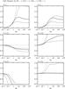	Fig. 3 Same as in Fig. 1 but for the case of salt-fingers, ∇μ < 0,∇ − ∇ad < 0, Rμ < 1.
In the text

	Fig. 4 The z-profile of the predicted passive tracer diffusivity vs. the values measured at NATRE.
In the text

References

- Aller, L. H., & Chapman, S. 1960, ApJ, 132, 1 [Google Scholar]
- Canuto, V. M. 1997, ApJ, 482, 827 [Google Scholar]
- Canuto, V. M. 1999, ApJ, 524, 311 (cited as C99) [NASA ADS] [CrossRef] [Google Scholar]
- Canuto, V. M. 2011, A&A, 528, A76, A77 (Papers I and II) [NASA ADS] [CrossRef] [EDP Sciences] [Google Scholar]
- Chapman, S., & Cowling, T. G. 1970, The mathematical theory of non uniform gases (Cambridge Univ. Press) [Google Scholar]
- Charbonnel, C., & Talon, S. 2005, Science, 309, 2189 [NASA ADS] [CrossRef] [PubMed] [Google Scholar]
- Charbonnel, C., & Talon, S. 2007, Science, 318, 922 [CrossRef] [PubMed] [Google Scholar]
- Charbonnel, C., & Zahn, J. P. 2007, A&A, 467, L15 [NASA ADS] [CrossRef] [EDP Sciences] [Google Scholar]
- Favre, A. 1969, in Problems of Hydrodynamics and continuous mechanics (Philadelphia: SIAM), 231 [Google Scholar]
- Ledwell, J. R., Watson, A. J., & Law, C. S. 1993, Nature, 364, 701 [NASA ADS] [CrossRef] [Google Scholar]
- Ledwell, J. R., Wilson, A. J., & Law, C. S. 1998, J. Geophys. Res., 103, 21499 [NASA ADS] [CrossRef] [Google Scholar]
- Michaud, G. 1970, ApJ, 160, 641 [NASA ADS] [CrossRef] [Google Scholar]
- Schatzman, E. 1969, A&A, 3, 331 [NASA ADS] [Google Scholar]
- St. Laurent, L., & Schmitt, R. W. 1999, J. Phys. Oceanogr., 29, 1404 [NASA ADS] [CrossRef] [Google Scholar]
- Vauclair, S., & Vauclair, G. 1982, ARA&A, 30, 3 [Google Scholar]