| Issue |
A&A
Volume 528, April 2011
|
|
|---|---|---|
| Article Number | A80 | |
| Number of page(s) | 4 | |
| Section | Astrophysical processes | |
| DOI | https://doi.org/10.1051/0004-6361/201014450 | |
| Published online | 04 March 2011 | |
Stellar mixing
V. Overshooting⋆
1
NASA, Goddard Institute for Space Studies,
New York, NY
10025,
USA
2
Department of Applied Physics and Applied Mathematics, Columbia
University, New York,
NY
10027,
USA
e-mail: This email address is being protected from spambots. You need JavaScript enabled to view it.
Received:
17
March
2010
Accepted:
10
October
2010
Abstract
Helio-seismological data suggest an overshooting (OV) extent of 0.07 Hp (Hp is the pressure scale height), while theoretical predictions from both models and numerical simulations yield values that are an order of magnitude higher. The reason identified by the authors of numerical simulations is the limited range of physical parameters allowed by the numerical simulations compared to the true solar values; specifically, the simulations are still too viscous. In the case of theoretical models, we discuss limitations that at present cannot be solved. For these reasons, we propose and work out a different methodology, which has in principle the following advantages. First, there is no longer a need to model the flux of turbulent kinetic energy, which has been a stumbling block for many years and whose modeling has introduced uncertainties that are difficult to control. Second, we account for processes not included before: shear (differential rotation), meridional currents, gravitational energy, stable-unstable stratification, and double diffusion.
Key words: turbulence / diffusion / convection / hydrodynamics / methods: analytical / stars: rotation
This work is dedicated to Aura Sofia Canuto.
© ESO, 2011
1. Formulation of the problem
Outside the unstably stratified CZ (convective cones) of stellar interiors there are dynamically important stably stratified regions referred to as OV (overshooting regions), which over the years have attracted a great deal of attention, and yet the true extent of such regions is still uncertain. In the solar case (Roxburgh 1978, 1989; Anderson et al. 1990; Spiegel & Zahn 1992), helio-seismological data suggest an OV extent of 0.05–0.1 Hp (Basu & Antia 1994; Basu et al. 1994; Thompson et al. 2003; Christensen-Dalsgaard et al. 2010), while theoretical predictions from both models (Xiong 1986; Deng & Xiong 2008) and numerical simulations (Brummet et al. 2002) yield results that are an order of magnitude greater. The similarity of the latter results may actually be coincidental since it is known that numerical simulations are still too viscous; for example, the Prandtl number is O(1) while the real value of O(10-8) and thus the numerical simulations do not yet resolve the full spectrum of eddies, while theoretical models are based on the assumption of infinite Reynolds numbers and thus account for all the eddies (for recent review of both methods, see Kupka 2008). This means not only that caution must be exercised in comparing the results of these different approaches but also that, should helio data be used for comparison, it must be kept in mind that they are derived under the assumption that the temperature gradient in the OV region is adiabatic. In our opinion, before a meaningful comparison is possible between; a) helio data; b) numerical simulations; and c) theoretical OV models, the last two must be improved internally, and in this paper we discuss method c) and suggest a reformulation of the procedure used thus far with the intent of overcoming the existing shortcomings.
The procedure used to compute the OV in method c), within the context of stellar structure-evolutionary codes, is to solve the stellar structure equations, together with a turbulence model (of variable complexity), where a key component is the equation for the eddy kinetic energy K. That is the formulation that we discuss. In general, the equation for K has the following form, see Paper I, Eqs. (7c)–(7f): 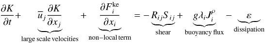 (1a)where shear Sij, Reynolds stresses Rij, buoyancy flux
  , and flux of kinetic energy
  are defined as
  (1b)Here,
  represent the heat and concentration fluxes (c is an arbitrary concentration field and αT = − ρ-1(∂ρ / ∂T)p,c, αc = + ρ-1(∂ρ / ∂c)p,T are the expansion coefficients). Several comments are in order concerning Eq. (1a). First, the second term on the lhs represents the advection of K by azimuthal and meridional currents
  whose structure and topology are only recently being revealed by helio-seismological data (Thompson et al. 2003; Mitra-Kraev & Thompson 2007; Gough & Hindman 2009). At present, such currents are not included in any OV model. Second, since − RijSij > 0, the first term on the rhs of (1a) represents the production of K by shear. Differential rotation is included in this term whose evaluation requires the knowledge of Rij, the Reynolds stresses whose general form was constructed in Papers I–III. No OV model has thus far included shear production. Third, the second and third terms on the rhs of (1a) represent the buoyancy flux that contains the possibility of DD processes (double diffusion: salt-fingers and semi-convection),whose effect we now study (Vauclair 2004, 2008; Charbonnel & Zahn 2007, and references cited there of previous work). Using the second of (1b), we have in the 1D case
  (1c)In the case of salt-fingers, the T-field is stable and the μ-field is unstable and the instability of the μ-field generates mixing. Since the process is characterized by the relations N2 > 0:Rμ < 1, ∇ − ∇ad < 0, we have
  (1d)in which case
  (1e)For semi-convection, the μ-field is stable and T-field is unstable and the instability of the T-field generates mixing. Since in this case the process is characterized by the relations N2 > 0: Rμ > 1, ∇ − ∇ad > 0, we have
  (1f)in which case
  (1g)As a result, both salt fingers and semi-convection generate a positive Jρ which acts like a source of K that increases the extent of the OV. Within this background, one must consider that all present formulations of the OV extent within method c) have adopted the following equation for K:
  (1h)which is the limit of (1a) in the case of no shear (no differential rotation), no meridional currents and no DD. The effect of DD processes is particularly interesting, since even without numerical estimates, one can understand qualitatively what the effect is on the extent of the OV. Without DD, in Eq. (1h) Jh < 0 and thus the buoyancy flux term in (1h) is negative and acts like a sink of K. As such it tends to decrease the extent of the OV. Since the whole rhs of (1h) is now negative, the only way to avoid (1h) from representing a case of decaying turbulence is to have a negative gradient of the non-local term flux of K denoted by , which represents the fourth problem represented by the need to model the third-order moment (TOM) in terms of some second-order moment. In their analysis, Xiong (1986) and Deng & Xiong (2008) adopted a down-gradient approximation, DGA, which, in the 1D case has the form
  (1i)
where Km is a momentum diffusivity. The problem of modeling TOMs was discussed in detail in Sect. 11 of Canuto (2009) where the relevant work by previous authors was discussed together with most recent advances. In spite of considerable progress in modeling TOMs documented in the work just cited, the present author is unable to suggest an expression for representative of the physical conditions characterizing the OV. This is because the assessments of the TOMs models were made using primarily planetary boundary layer processes that lack many key stellar features, such as meridional currents, differential rotation, radiative losses, and double-diffusion.
(1i)
where Km is a momentum diffusivity. The problem of modeling TOMs was discussed in detail in Sect. 11 of Canuto (2009) where the relevant work by previous authors was discussed together with most recent advances. In spite of considerable progress in modeling TOMs documented in the work just cited, the present author is unable to suggest an expression for representative of the physical conditions characterizing the OV. This is because the assessments of the TOMs models were made using primarily planetary boundary layer processes that lack many key stellar features, such as meridional currents, differential rotation, radiative losses, and double-diffusion.
The reliability of the DGA closure (1i) in a stellar context is uncertain, to say the least, and yet the extent of the OV depends crucially on the structure of . Several studies have shed light on the more general problem of the TOMs. The most extensive studies are those by Kupka & Muthsam (2007, 2008) and Kupka (2008), the general conclusion of which is that the DGAs rarely ever work, and if they do so, it is only near the boundary of convection zones. Due to these shortcomings, the key suggestion here is to abandon attempts at modeling  and instead construct a differential equation for vs. radius. The point at which such flux has decreased to say 1% of its value at the bottom of the CZ can be considered a good measure of the OV extent. In the new procedure, we further include
-
a)
the effect of meridional currents,
-
b)
the flux of the total energy E;
-
c)
the flux of the Reynolds stresses; and
-
d)
the effect of unstable-stable stratification, differential rotation, shear, radiative losses (Peclet number), and double diffusion.
2. New approach
We consider the energy conservation law (I, Eq. (4a) with 
 (2a)where
  (2b)which represents the total energy of the system given by the
sum of enthalpy cpT, turbulent kinetic
energy K, mean flow (meridional and azimuthal) kinetic energy
KM, and gravitational energy G. Furthermore,
we have the total flux given by
(2b)which represents the total energy of the system given by the
sum of enthalpy cpT, turbulent kinetic
energy K, mean flow (meridional and azimuthal) kinetic energy
KM, and gravitational energy G. Furthermore,
we have the total flux given by 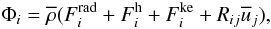 (2c)which represents the sum of the radiative, heat, and
turbulent kinetic energy fluxes as well as the flux of the Reynolds stresses by the mean
flow, where
(2c)which represents the sum of the radiative, heat, and
turbulent kinetic energy fluxes as well as the flux of the Reynolds stresses by the mean
flow, where  (2d)where χr is the thermometric
conductivity with units of cm2 s-1. Next, we consider Eqs. (I, 5) for
the mean concentration:
(2d)where χr is the thermometric
conductivity with units of cm2 s-1. Next, we consider Eqs. (I, 5) for
the mean concentration:  (3a)where
  . The variables
  and χc are
the physical equivalents of
and χc are
the physical equivalents of  and χr. We
must note that χc is often called D in the
literature, e.g., Michaud (1970, Eq. (1)) and Vauclair & Vauclair (1983, Eq. (1)).
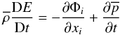
Multiplying Eqs. (2a) and (3a) by
αT,αc, respectively, and
subtracting the two, one obtains an equation of the same structure of (2a), namely,
and χr. We
must note that χc is often called D in the
literature, e.g., Michaud (1970, Eq. (1)) and Vauclair & Vauclair (1983, Eq. (1)).
Multiplying Eqs. (2a) and (3a) by
αT,αc, respectively, and
subtracting the two, one obtains an equation of the same structure of (2a), namely,  (3b)where
 ![Mathematical equation: % subequation 953 2 \begin{equation} \label{eq15} E_\ast =c_{\rm p} [\alpha _T T(1+\xi )-\alpha _c C],\, \xi =\frac{K+K_{\rm M} +G}{c_{\rm p} T}, \, \overline {p_\ast } = \alpha _T \overline p \end{equation}](/articles/aa/full_html/2011/04/aa14450-10/aa14450-10-eq50.png) (3c)
(3c) (3d)where for brevity we call
  the radiative–molecular terms:
 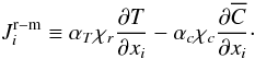 (3e)Clearly, the variable ξ represents the
ratio of the sum of the turbulent energy K, the mean flow energy
KM, and the gravitational energy to the thermal energy. The
first four terms in (3d) represent the
turbulent fluxes of buoyancy, eddy kinetic energy, radiative-molecular fluxes. The last term
represents the flux of the Reynolds stresses
Rij by the large-scale fields . In the stationary limit, Eqs. (3b)–(3d) reduce to the
following generalized flux conservation law:
(3e)Clearly, the variable ξ represents the
ratio of the sum of the turbulent energy K, the mean flow energy
KM, and the gravitational energy to the thermal energy. The
first four terms in (3d) represent the
turbulent fluxes of buoyancy, eddy kinetic energy, radiative-molecular fluxes. The last term
represents the flux of the Reynolds stresses
Rij by the large-scale fields . In the stationary limit, Eqs. (3b)–(3d) reduce to the
following generalized flux conservation law:  (4a)We note that each term in (4a) has the units of
[αTu3]. The
“traditional” flux conservation law used in stellar models contains only the first and the
radiative parts, in which case Eq. (4a)
reduces to
(4a)We note that each term in (4a) has the units of
[αTu3]. The
“traditional” flux conservation law used in stellar models contains only the first and the
radiative parts, in which case Eq. (4a)
reduces to  (4b)which expresses the constancy of the convective plus
radiative fluxes. Eliminating the buoyancy flux between Eqs. (1a) and (4a), we obtain a
differential equation for :
(4b)which expresses the constancy of the convective plus
radiative fluxes. Eliminating the buoyancy flux between Eqs. (1a) and (4a), we obtain a
differential equation for :  (5a)where we have used the notation
  (5b)Each term of Eq. (5a) has the units of a dissipation
[L2 / t3]. If one keeps only
Φold, Eq. (5a) coincides with
the equation originally suggested by Roxburgh (1978).
Since the constant C is related to the total stellar luminosity, the final criterion is
expressed in terms of the integral of the difference
L(N) − L(r) between
the nuclear and radiative luminosities. Since such a difference is positive in the
convective zone CZ and negative in the OV, the integral changes sign at some distance
r∗ that was identified with the OV extent. The presence of the
new term Φnew in (5a) introduces
the following new features
(5b)Each term of Eq. (5a) has the units of a dissipation
[L2 / t3]. If one keeps only
Φold, Eq. (5a) coincides with
the equation originally suggested by Roxburgh (1978).
Since the constant C is related to the total stellar luminosity, the final criterion is
expressed in terms of the integral of the difference
L(N) − L(r) between
the nuclear and radiative luminosities. Since such a difference is positive in the
convective zone CZ and negative in the OV, the integral changes sign at some distance
r∗ that was identified with the OV extent. The presence of the
new term Φnew in (5a) introduces
the following new features  (5c)The solution of the new equation for the flux
of K, Eq. (5a) can only
be carried out in conjunction with a model for the Reynolds stresses, which we have
discussed in Papers II and III. One also needs a stellar code to provide the radiative flux
(5c)The solution of the new equation for the flux
of K, Eq. (5a) can only
be carried out in conjunction with a model for the Reynolds stresses, which we have
discussed in Papers II and III. One also needs a stellar code to provide the radiative flux  . Finally, one must model the
dissipation ε, a topic that we discussed in Papers I and II and which we
slightly amplify here by listing some new options.
. Finally, one must model the
dissipation ε, a topic that we discussed in Papers I and II and which we
slightly amplify here by listing some new options.
-
a)
The most obvious choice consists of adopting a Kolmogorovtype law,
 (5d)where ℓ is a dissipation scale. In a
stably stratified regime, such as the one encountered in a stellar radiative zone, the
validity of the Kolmogorov spectrum is questionable and though one can formally
write (5d), it is of little help
since ℓ turns out to be a rather complex function of the stability
functions such as the flux Richardson number (Cheng & Canuto 1994). This option is not advisable because it introduces a
variable that is difficult to control.
(5d)where ℓ is a dissipation scale. In a
stably stratified regime, such as the one encountered in a stellar radiative zone, the
validity of the Kolmogorov spectrum is questionable and though one can formally
write (5d), it is of little help
since ℓ turns out to be a rather complex function of the stability
functions such as the flux Richardson number (Cheng & Canuto 1994). This option is not advisable because it introduces a
variable that is difficult to control. -
b)
Following Paper II, Eq. (10a), one can identify ε with the estimate provided by the internal gravity waves model (IGW)
 (5e)which in the solar case applies to the radiative zone
below the convective zone, but which may be nontrivial to extend to other stars.
(5e)which in the solar case applies to the radiative zone
below the convective zone, but which may be nontrivial to extend to other stars. -
c)
The most reliable procedure is probably the one discussed in Sect. 6 of Paper I, which calls for the solution of the following differential equation for ε (c1,2 = 2.88, 3.84)
 (5f)
(5f)
 (5g)The presence of in (5f)
means that the latter must be solved with Eqs. (5a), (5b). Even this procedure still
requires the knowledge of one variable, the dissipation time scale τ. Since
we no longer have an independent differential equation for the latter (since we have used
both the K and ε equations), we suggest a parametric form
consisting of assuming that in stably stratified flows:
(5g)The presence of in (5f)
means that the latter must be solved with Eqs. (5a), (5b). Even this procedure still
requires the knowledge of one variable, the dissipation time scale τ. Since
we no longer have an independent differential equation for the latter (since we have used
both the K and ε equations), we suggest a parametric form
consisting of assuming that in stably stratified flows:  (5h)Admittedly, this introduces a proportionality constant of
order unity in (5h), but we consider this a
far more physically justified and general procedure than the previous choices.
(5h)Admittedly, this introduces a proportionality constant of
order unity in (5h), but we consider this a
far more physically justified and general procedure than the previous choices.
Once Eqs. (5a), (5b) are solved with (5f), the OV extent in the radiative zone can be obtained as the distance from the bottom of the CZ where the flux of the kinetic energy has decreased, to say, 1% of its value at the bottom of the CZ.
Since we have eliminated the buoyancy flux that no longer appears explicitly in (5a), one may wonder about the effect of DD on the extent of the OV.
3. Physical interpretation of the new term Φnew
The novel feature in (5a) is represented by Φnew, which brings about features that were not accounted for before and which we now analyze. The first term in Φnew represents the production of kinetic energy by shear:  (6a)The second term represents the flux by the mean currents of the total energy of the system
  (6b)while the third term represents the flux of the Reynolds stresses by the mean currents
  (6c)which we now analyze separately. Using the results presented in Paper IV, we have
  (7a)where (here r is the radial distance):
  (7b)where the structure function Sm was plotted in Fig. 2 of Paper IV. Next, we consider the second term in Φnew, which is given by
  (8)Since the available data on the meridional currents by Mitra-Kraev & Thompson (2007) and Gough & Hindman (2009) do not extend below the convective zone, we are unable at present to determine the size of this term. The third term is given by
  (9a)where the dynamic equations for the meridional velocities
  are given by Eqs. (8) of Paper IV. If we assume that the second term in the last expression on the rhs of (9) is the largest, we then have, with
  :
:  (9b)where
  (9c)
(9c)
4. Conclusions
In this paper we have put forward the suggestion of abandoning the canonical attempt to solve Eq. (1a) which requires a model for the flux of kinetic energy ; see Eq. (1i) and discussion thereafter, for which the present models are neither unique nor fully trustworthy. Rather, we suggest viewing the latter function as an unknown to be determined by solving the differential equation, Eq. (5a). The previous form of (5a) suggested by Roxburgh (1978) did not include the new term Φnew, which brings the following new features:
-
a)
the effect of meridional currents,
-
b)
the flux of the total energy E,
-
c)
the flux of the Reynolds stresses and
-
d)
a full model of the Reynolds stresses that accounts for stable stratification, unstable stratification, differential rotation, shear, radiative losses (Peclet number) and double diffusion.
References
- Anderson, J., Nordstrom, B., & Clausen, J. V. 1990, ApJ, 363, L33 [NASA ADS] [CrossRef] [Google Scholar]
- Antia, H. M., Basu, S., & Chitre, S. M. 1998, MNRAS, 298, 543 [NASA ADS] [CrossRef] [Google Scholar]
- Basu, S., & Antia, H. M. 1994, MNRAS, 269, 1137 [NASA ADS] [Google Scholar]
- Basu, S., Antia, H. M., & Narashima, D. 1994, MNRAS, 267, 209 [NASA ADS] [CrossRef] [Google Scholar]
- Brummell, N. H., Clune, T. L., & Toomre, J. 2002, ApJ, 570, 825 [Google Scholar]
- Canuto, V. M. 2006, Convection in Astrophysics, ed. F. Kupka, I. W. Roxburgh, K. L. Chan, Part I, page 3 and Part II, IAU Symp., 239, 19 [Google Scholar]
- Canuto, V. M. 2009, Turbulence in astrophysical and geophysical flows, in Interdisciplinary Aspects of Turbulence, Springer Lectures Notes in Physics, ed. W. Hillebrandt, & F. Kupka (Berlin: Springer and Verlag), 756, 107 [Google Scholar]
- Canuto, V. M., Howard, A. M., & Cheng, Y. 2008, Geophys. Res. Lett., 35, L02613 [Google Scholar]
- Charbonnel, C., & Zahn, J. P. 2007, A&A, 467, L15 [NASA ADS] [CrossRef] [EDP Sciences] [Google Scholar]
- Cheng, Y., & Canuto, V. M. 1994, J. Atmos. Sci., 51, 2384 [NASA ADS] [CrossRef] [Google Scholar]
- Christensen-Dalsgaard, J., Monteiro, M. J. P. F. G., Rempel, M., & Thompson, M. J. 2010, MNRAS, accepted [Google Scholar]
- Deng, L., & Xiong, D. R. 2008, ed. L. Deng, & K. L. Chan (Cambridge Univ. Press), IAU Symp., 252, 83 [Google Scholar]
- Gough, D., & Hindman, B. W. 2010, ApJ, 714, 960 [NASA ADS] [CrossRef] [Google Scholar]
- Kupka, F. 2008, ed. L. Deng, & K. L. Chan (Cambridge Univ. Press), IAU Symp., 252, 451 [Google Scholar]
- Kupka, F., & Muthsam, H. J. 2007, ed. F. Kupka, I. W. Roxburgh, & K. L. Chan (Cambridge Univ. Press), IAU Symp., 239, 83 [Google Scholar]
- Kupka, F., & Muthsam, H. J. 2008, ed. L. Deng, & K. L. Chan (Cambridge Univ. Press), IAU Symp., 252, 463 [Google Scholar]
- Mitra-Kraev, U., & Thompson, M. J. 2007, Astron. Nachr., 328, 10, 1009 [NASA ADS] [CrossRef] [Google Scholar]
- Roxburgh, I. W. 1978, A&A, 65, 281 [NASA ADS] [Google Scholar]
- Roxburg, I. W. 1989, A&A, 211, 361 [NASA ADS] [Google Scholar]
- Spiegel, E. A., & Zahn, J. P. 1992, A&A, 265, 106 [NASA ADS] [Google Scholar]
- Thompson, M. J. J., Christensen-Dalsgaard, M. S. M., & Toomre, J. 2003, ARA&A, 41, 599 [NASA ADS] [CrossRef] [Google Scholar]
- Vauclair, S. 2004, ApJ, 605, 874 [NASA ADS] [CrossRef] [Google Scholar]
- Vauciar, S. 2008, in ed. L. Deng, & K. L. Chan (Cambridge Univ. Press), IAU Symp., 252, 83, 97 [Google Scholar]
- Xiong, D. R. 1986, A&A, 167, 239 [NASA ADS] [Google Scholar]
Current usage metrics show cumulative count of Article Views (full-text article views including HTML views, PDF and ePub downloads, according to the available data) and Abstracts Views on Vision4Press platform.
Data correspond to usage on the plateform after 2015. The current usage metrics is available 48-96 hours after online publication and is updated daily on week days.
Initial download of the metrics may take a while.