| Issue |
A&A
Volume 528, April 2011
|
|
|---|---|---|
| Article Number | A76 | |
| Number of page(s) | 9 | |
| Section | Astrophysical processes | |
| DOI | https://doi.org/10.1051/0004-6361/201014447 | |
| Published online | 04 March 2011 | |
Stellar mixing
I. Formalism⋆
1 NASA, Goddard Institute for Space
Studies, New
York, NY 10025, USA
2 Department of Applied Physics and
Applied Mathematics, Columbia University, New York, NY
10027,
USA
e-mail: This email address is being protected from spambots. You need JavaScript enabled to view it.
Received: 17 March 2010
Accepted: 25 August 2010
Abstract
In this paper we use the Reynolds stress models (RSM) to derive algebraic expressions for the following variables: a) heat fluxes; b) μ fluxes; and c) momentum fluxes. These relations, which are fully 3D, include:
1) stable and unstable stratification, represented by the Brunt-Väisäla frequency,  ;
;
2) double diffusion, salt-fingers, and semi-convection, represented by the density ratio Rμ = ∇μ(∇ − ∇ad)-1;
3) shear (differential rotation), represented by the mean squared shear Σ2 or by the Richardson number, Ri = N2Σ-2;
4) radiative losses represented by a Peclet number, Pe;
5) a complete analytical solution of the 1D version of the model. In general, the model requires the solution of two differential equations for the eddy kinetic energy K and its rate of dissipation, ε. In the local and stationary cases, when production equals dissipation, the model equations are all algebraic.
Key words: turbulence / diffusion / convection / hydrodynamics / methods: analytical / stars: rotation
This work is dedicated to Aura Sofia Canuto.
© ESO, 2011
1. Introduction
Since mixing in stars is a complex interplay of regimes of unstable stratification, stable stratification, differential rotation, gravity waves, double-diffusion, etc., it could be expected that the formalisms employed are general enough to account for such a wide variety of processes. And yet, the literature shows that this is not the case since the two main methodologies being employed are: a) large scale numerical simulations (e.g., Brummell et al. 2002); and b) heuristic models (e.g., Maeder & Meynet 2001; Mathis et al. 2004; Palacios et al. 2003, 2006; Charbonnel & Talon 2005, 2007).
In the first case, the values of some of the stellar parameters, such as the Prandtl number, are widely different from those in stars, and no specific results have yet been produced that can be employed in stellar structure/evolution calculations. The authors of those studies in fact state that their primary goal was to elucidate the intertwined physical processes and not (yet) to provide stellar studies with tools to model the processes of interest. As for the heuristic models, we believe they may have exhausted their fruitfulness since it is extremely difficult, if not almost impossible, to build models capable of embracing the wide variety of processes such as the ones cited at the beginning, ultimately because such processes are not additive.
It is instructive to point out that an analogous situation once existed in geophysics, specifically in modeling atmospheric and oceanic mixing. A few decades ago, however, a shift took place from heuristic, unpredictive approaches in favor of a predictive, prognostic, and flexible tool known as RSM (Reynolds stress models), which are now commonly used. For reasons unclear to the present author, stellar mixing studies have lagged behind geophysical studies, and this paper will thus present a new RSM-based model, as well as the limitations of the heuristic models.
The RSM consist of a set of equations for the turbulent correlations of the velocity, temperature, and concentration fields that are derived directly from the Navier-Stokes, temperature, and concentration equations. The main features can be summarized as follows:
-
a)
mathematical structure: most of the relevant equations arelinear, algebraic relations and thus pose no particular numericalproblems;
-
b)
flexibility: one of the key advantages is that adding new processes such as rotation, vorticity, double-diffusion, etc., does not require guesswork since the RSM have a well-defined set of procedural rules,
-
c)
assessment: the results of the RSM can be assessed before they are used in a stellar context, an important feature that none of the heuristic model enjoys, raising the justified suspicion that such models, tailored to a specific astrophysical setting, have a limited predictive power. The general properties of the RSM have recently been reviewed in (Canuto 2006, 2009).
2. Mean variables
When dealing with mixing in stellar interiors, most of the models concentrate on the temperature field because it enters the convective flux. However, a single field such as the temperature, cannot represent the complexity of stellar mixing processes for which one needs three fields,  (1a)representing velocity, temperature, and a scalar c-field. The velocity field is needed because its mean values correspond to meridional and azimuthal currents, while its gradients give rise to shear (differential rotation) mixing. The scalar c-field can be of two kinds: active and passive. An active c-field is, for example, the mean molecular weight
  , and a passive c-field is for example a tracer such as Li7. By active is meant a scalar that affects the density, which in turn affects the velocity field, and thus ultimately alters the turbulent state; in contrast, a passive scalar is transported by the flow without altering it. This can be seen by considering the relations
  (1b)where αT,μ = − (∂lnρ / ∂T)p,μ,(∂lnρ / ∂μ)p,T are the expansion coefficients. A passive scalar does not contribute to the rhs of (1b). When we expand the density field in the derivations, we use (1b) in which the c-field is the μ-field. Their different effects on the density mean that the two c-fields have different dynamics, and in what follows we use the c-field notation when the relations apply to both passive and active scalars. When the differentiation becomes necessary, we use the symbol
  for an active scalar. The inclusion of the field is necessary since its gradient is opposite to that of the T-field, a situation that in the ocean gives rise to two well known processes, namely salt-fingers and diffusive convection, the latter being called semi-convection in the astrophysical literature. Each field has an average and a fluctuating component,
  (1c)and since due to turbulence, the correlation among two fluctuating variables is not zero, in addition to having three equations for the mean fields
  , one must derive the equations for second-order correlations, such as
  (1d)However, it turns out that the equations for the fluxes (1d) involve the correlations of the fields themselves, specifically
  (1e)whose dynamic equations must therefore also be included and solved. In what follows, we first derive the dynamic equations for the three mean variables
  and then derive those for the variables (1c, d).
2.1. Mean temperature
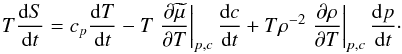
Since there is no conservation equation for T, we begin with the entropy S-equation from which one then derives an equation for T. Second, we must consider an entropy equation for a mixture of fluids since we want to include different species, for example He and H. With these provisos, the starting S-equation reads as (Landau & Lifshitz 1987)  (2a)where we have defined the following variables:
  (2b)where ui is the total velocity field, ν the kinematic viscosity, ρ the density, and σij the viscous stress tensor. Assuming incompressibility requires that the last term in (2b) is zero. Furthermore, the q-flux is defined as follows:
 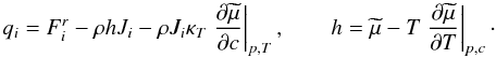 (2c)here,
  is the radiative flux which, in the absence of the diffusion flux Ji, would be the only term in qi and
  is the chemical potential of the mixture. In a two-fluid model, the densities of the two components are ρc,ρ(1 − c), respectively and the concentration equation reads as
 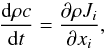 (2d)when the c-field corresponds for example to Li7, the corresponding diffusion flux Ji discussed by Chapman & Cowling (1970), is given by
 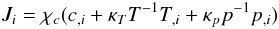 (2e)with the standard notation a,i = ∂a / ∂xi, and where κT,κp are dimensionless functions. Often, in the literature Ji includes the density and has the opposite sign, and χc is called D. We have also found that different authors employed different notations, for example Eq. (2.1) of Aller & Chapman (1960), Eq. (3) of Schatzman (1969), Eq. (1) of Michaud (1970), and Eq. (1) of Vauclair & Vauclair (1982). As one can observe from Eq. (2e), the diffusion flux is contributed not only by the first term, which is the traditional gradient of the concentration, but also by the temperature and pressure gradients first introduced by Chapman (1917). Next, one employs the thermodynamic relations:
 (3a)Making use of Eq. (2d) and taking
  corresponding to no radiation pressure, Eq. (2a) becomes
 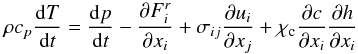 (3b)where we have neglected a term that involves the product of two molecular diffusivities and where
  (3c)where the μ are the mean molecular weights of the two substances. We note that if one employs an equation of state for a perfect gas, the dp/dt term inf (3b) can be absorbed into the left hand side which retains the same form but with cv in lieu of cp. The next step is to employ (1b), separate all the fields into a mean and a fluctuating part, carry out the averages, and obtain the dynamic equation for the mean variables. The necessary steps were discussed in a previous work (Canuto 1999), so we limit ourselves to cite the final result that reads as
 (4a)where
 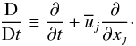 (4b)On the lefthand side of (4a), we have defined the following variables:
 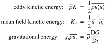 (4c)On the right side of (4a), we have the variables:
  (4d)where Kr = cpρχ and χ, the thermometric conductivity, has the units of cm2 s-1. The diffusion approximation in the first of (4d) is not required by the present formalism and is being suggested as an example. At first sight, Eq. (4a) may be somewhat surprising since one is accustomed to the much simpler equation
 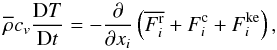 (4e)which in the stationary case further reduces to the “flux conservation law”:
 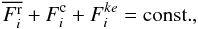 (4f)implying the constancy of the radiative + convective + eddy kinetic energy fluxes, the latter being often neglected. Equation (4a) is considerably more general than (4f) for the following reasons:
- 1)
the lhs contains the total energy of the system, as indeedexpected, namely,
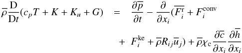
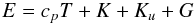 (4g)which is the sum of enthalpy, turbulent kinetic energy, mean flow kinetic energy and gravitational energy, respectively. Which of the four terms in (4g) is the largest depends on the specific physical problem at hand;
 in the second term of the rhs of (4a), we have four terms
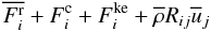 (4h)which represent the radiative, convective, and eddy kinetic energy fluxes, while the last term is the flux of the Reynolds stresses by the large scale velocity field
  . To get a feeling for what the last term means, consider the z-component of (4h) and the closures to be derived in what follows:
 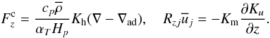 (4i)Here, Kh,m are heat and momentum diffusivities, Ku the mean flow kinetic energy (see the second of 4c) and we have used the relations:
 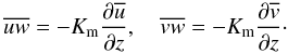 (4j)Thus, the ratio of the second to last term in (4h) is given by
 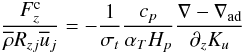 (4k)where the ratio Kh/Km is the inverse of the turbulent Prandtl number σt, which in the case of stable stratification ∇−∇ad < 0, is an increasing function of the Richardson number as discussed in detail in Paper II. To assign a numerical value to the mean kinetic energy, one needs the meridional currents possibly derived from helio-seismological studies, as discussed in Paper V;
 an interesting but never accounted for term, is the last one in (4a) which represents the effect of the gradient of the mean c-field on the temperature field.
2.2. Mean c-field
The starting relation is Eqs. (2d, e). Carrying out the mass averaging process (Favre 1969; Canuto 1997) defined as  (5a)we obtain
  (5b)The second term in the rhs of (5b) is the ordinary molecular diffusion, while the first term is turbulent c-flux akin to the convective flux, second term in (4d):
  (5c)At first sight, it may look as though Eqs. (5b, c) are unrelated to the T-field but that is not the case since, as we show below in Eqs. (12d, e), the turbulent c-flux (5c) entails the turbulent convective flux. Clearly, the term in (5b) with the molecular diffusivity χc only represents passive scalars.
2.3. Mean velocity
We begin with the Navier-Stokes equations for a compressible fluid:  (6a)where the viscous stress tensor was defined in Eq. (2b). Mass averaging Eq. (6a) via relations analogous to (5a)
  (6b)one obtains from (6a):
  (6c)where the Reynolds stresses were defined in Eq. (4d). It is important to notice that Eq. (6c) can be rewritten in the more transparent form:
 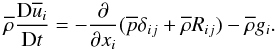 (6d)To solve Eq. (6d) one needs the Reynolds stresses, which we study in Sect. 3. In conclusion, the equations for the mean
  are given by Eqs. (4a), (5b), and (6d). These equations contain the following second-order turbulent correlations:
 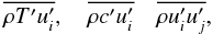 (6e)representing temperature, c-field, and momentum fluxes whose equations we derive next.
3. Reynolds stresses
The derivation of the dynamic equation for the Reynolds stress was presented in an earlier work (Canuto 1997, Eqs. (14)), so we only cite the final result which we simplify by neglecting the terms due to compressibility. We have 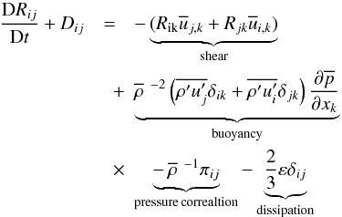 (7a)where
 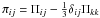 is the traceless pressure correlation tensor, and Dij represents the diffusion of the Reynolds and pressure fluxes, both of which are third-order moments. The trace of (7a) yields the equation for the turbulent kinetic energy,
  (7b)which reads as
 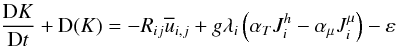 (7c)where
 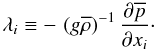 (7d)Since the density field depends on both T and μ-fields, we also have
 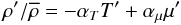 (7e)where αT,μ = − (∂lnρ / ∂T)p,μ,(∂lnρ / ∂μ)p,T are the expansion coefficients. Thus, the combination of heat and μ-fluxes:
 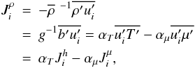 (7f)is called the density-buoyancy flux where
  is the buoyancy field. Thus, the physical interpretation of the rhs of (7c) is as follows. The first term is the source of K due to mean shear; the second term given by (7f) may act as a source or as a sink depending on whether one deals with unstable or stable stratification, as well as the sign of the μ gradient (in the case of salt fingers; the contribution is a source while in the diffusive convective case, semi-convection, the term acts as a sink); finally, the last term, which is always negative, represents the sink of K due to molecular viscosity, and its equation will be discussed in Sect. 6.
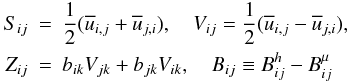
Next, we consider the Reynolds stresses which enter the first source term in the rhs of (7c), and we introduce the traceless form  (8a)whose dynamic equation can be derived from Eqs. (7a, c) to be
  (8b)where we have defined the following tensors with zero trace:
  (8c)
(8c) (8d)
(8d) (8e)The final step is the closure of the pressure correlation tensor, a topic that has been widely discussed elsewhere (Canuto 1994, 1997) and need not be repeated here. The final expression of Eq. (8b) is then
  (8f)Since α1,2 = 0.984,0.568, β5 = 1 / 2,τpv = 2τ / 5, we neglect the Σij term and round off α2 = 1 / 2, in which case (8f) simplifies to
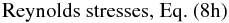
  (8g)which, in the stationary and local limit, becomes
  (8h)Equation (8h) is quite simple: in fact, it is a set of linear algebraic relations whose solution yields the Reynolds stresses bij. We recall that Zij depends on bij itself, and Bij are given in Sect. 4. We also recall that the dynamical time scale is given by
  (8i)whose determination we discuss in Sect. 6.
4. Heat and μ-fluxes
We begin by defining the heat and μ-fluxes:
 To derive the dynamic equation for (9a), one begins with Eq. (3b) multiplied by ui and adds to it Eq. (6a) multiplied by T. Neglecting the molecular terms, we have
  (9c)where the variable A is defined as
  (9d)Next, we average Eqs. (9c, d). The process was carried out in detail elsewhere (Canuto 1997) with the result
 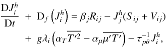 (9e)where
 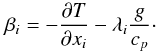 (9f)It is useful to consider the physical origin of the third term on the rhs of (9e). Consider the fluctuating component of the term – ρg on the rhs of the momentum Eq. (6a). Since to obtain the dynamical equation for the heat flux (9a), one multiplies the T′ equation by
  and the equation by T′, the last operation gives rise to the term
 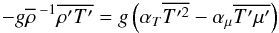 (9g)where we use (7e). Relation (9g) is indeed the third term in the rhs of (9e). The first term in the rhs of (9e) represents the potential energy (temperature variance), but due to the μ-field, there is a second term representing the correlation between the T and μ fields. In the local and stationary case, Eq. (9e) simplifies considerably as it becomes an algebraic equation for the heat flux:
  (9h)The last two terms can be derived to have the following form:
  (9i)Once substituted in (9h), the latter can be rewritten in the simpler form:
 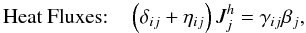 (10a)where we have defined the following tensors:
 ![Mathematical equation: % subequation 1674 1 \begin{eqnarray} \label{eq51} \gamma _{ij} &=& \pi _4 \tau (R_{ij} -\pi _2 g\alpha_\mu^\tau \lambda _i J_j^\mu ) \nonumber\\ \eta _{ij} &=&\pi _4 \tau [S_{ij} +V_{ij} -g\tau \lambda _i (\pi _5 \alpha _T \beta _j +\pi _2 \alpha _\mu \overline \mu _{,j} )]. \end{eqnarray}](/articles/aa/full_html/2011/04/aa14447-10/aa14447-10-eq121.png) (10b)In order to homogenize the notation, we have measured the different time scales in units of (8i) and introduced the following dimensionless variables,
(10b)In order to homogenize the notation, we have measured the different time scales in units of (8i) and introduced the following dimensionless variables,  (10c)whose determination is an important task that will be dealt with subsequently. Relations (10c) represent decay times due to smallscale dissipation as well as pressure-correlations time scales (hence the labels “pθ” and “pμ”), which in the turbulence closure literature are known as the Rotta’s (1951) terms. Some comments are needed to interpret the physical content of Eqs. (10a,b). The heat flux depends on the following variables:
  (10d)The Reynolds stresses Rij are obtained solving Eqs. (8h), which in turn depend on the density flux, that is, heat fluxes (10a, b) and concentration fluxes that we study next. It is of interest to note that the heat flux in (10a) can be rewritten in the more familiar form given by a heat diffusivity times the adiabatic temperature gradient. Indeed, using the Hamilton-Cayley theorem, one can rewrite (10a) as
 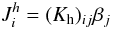 (10e)where (Kh)ij is a turbulent heat diffusivity tensor whose explicit form can be computed, but it is doubtful whether in practical computations such a form could be more useful than (10a).
 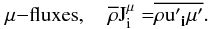 We begin with relations (2d, e). Multiplying (2d) by ui, Eq. (6a) by μ and adding the two, we obtain
 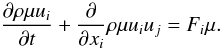 (11a)Next, using (5a), we mass average (11a) and obtain an equation analogous to (9c):
 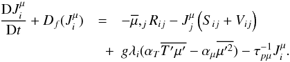 (11b)Using the second of (9i) and the analog of the first of (9i)
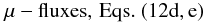
  (12a)we obtain, after some algebra, the following equation for the μ-flux:
  (12b)where
 ![Mathematical equation: % subequation 1831 2 \begin{eqnarray} \label{eq58} d_{ij} &=& \pi _1 \tau \left(R_{ij} + g \alpha _T \pi _2 \tau \lambda _i J_j^h \right) \nonumber \\ \xi _{ij} & = & \pi _1 \tau \left[S_{ij} +V_{ij} - g \tau \lambda _i \left(\pi _2 \alpha _T \beta _j +\pi _3 \alpha _\mu \overline \mu _{,j}\right) \right]. \end{eqnarray}](/articles/aa/full_html/2011/04/aa14447-10/aa14447-10-eq134.png) (12c)As discussed before, Eqs. (10a, b) and (12d, e) show that the heat and μ-fluxes depend on each other and both depend on shear and vorticity. In principle, Eqs. (12d, d) can also be written in a form analogous to Eq. (10e).
(12c)As discussed before, Eqs. (10a, b) and (12d, e) show that the heat and μ-fluxes depend on each other and both depend on shear and vorticity. In principle, Eqs. (12d, d) can also be written in a form analogous to Eq. (10e).
5. The dissipation-relaxation time scales π′s
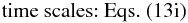
Each of the second-order correlations discussed in the previous sections is characterized by a dissipation-correlation time scale that we have normalized with the dynamical time scale (8i) giving rise to (10c), which must now be determined in terms of the large scale features of the model. Since we are considering a physical situation with both mean velocity fields (giving rise to shear mixing), temperature and μ- fields (giving rise to double-diffusion processes), we need two large-scale, dimensionless variables, one to characterize the temperature-velocity fields and the second to characterize the temperature-μ fields, or, more correctly, the relative gradients of these fields. Traditionally, these two variables have been chosen to be the Richardson number Ri and the density ratio Rμ (a term borrowed from oceanography). Ri is defined as  (13a)where Σ2 is the mean shear squared defined in terms of the mean velocities fields,
  (13b)while the Brunt-Väisäla frequency N is given by
 ![Mathematical equation: % subequation 1903 2 \begin{equation} \label{eq61} N^2= -\frac{g}{\rho} \frac{\partial \overline \rho }{\partial z}= g\alpha _T \left[\frac{\partial \overline T }{\partial z}-\left(\frac{\partial \overline T }{\partial z}\right)_{\rm ad} \right] - g \alpha _\mu \frac{\partial \overline \mu }{\partial z}, \end{equation}](/articles/aa/full_html/2011/04/aa14447-10/aa14447-10-eq142.png) (13c)where
(13c)where  are the expansion coefficients. Using the relations
 ![Mathematical equation: % subequation 1903 3 \begin{eqnarray} \label{eq62} \alpha_T \left[ -\frac{\partial \overline T}{\partial z} + \left(\frac{\partial \overline T}{\partial z}\right)_{\rm ad} \right]&=&H_p^{-1} (\nabla -\nabla _{\rm ad} ) \\[2.5mm] \label{eq63} \alpha _\mu \frac{\partial \overline \mu}{\partial z} &=& - H_p^{-1} \nabla_\mu, \quad \nabla _\mu \equiv \frac{\partial \ln \mu }{\partial \ln P}\cdot \end{eqnarray}](/articles/aa/full_html/2011/04/aa14447-10/aa14447-10-eq144.png) the density ratio is defined as
the density ratio is defined as  (13f)Equation (13c) then becomes
  (13g)The task is now that of constructing the functions
  (13h)The determination of such functions was the main goal of Canuto et al. (2008b, 2009) intended to reproduce laboratory data (without shear but with double-diffusion, DD) and oceanic data (which depend on both shear and DD instabilities). However, in a stellar context, one must include a Peclet number dependence because radiative losses by the eddies weaken the strength of turbulence. Adopting the treatment developed elsewhere (Canuto & Dubovikov 1998; Canuto et al. 2008a,b), we now have:
 ![Mathematical equation: % subequation 1903 7 \begin{eqnarray} \label{eq67} \pi _1 &=& \pi _1^0 \left(1+\frac{{\rm Ri}~R_\mu}{a + R_\mu } \right)^{-1},\,\, \pi _4 = \pi_4^0 f({\rm Pe})\left(1 + \frac{\rm Ri}{1 + a R_\mu}\right)^{-1} \nonumber\\ \pi _2 &=& \pi _2^0 (1 + {\rm Ri})^{-1}[1+ 2 {\rm Ri}\,R_\mu (1 + R_\mu ^2)^{-1}], \,\, \pi _5 = \pi _5^0 g({\rm Pe}), \nonumber\\ \pi _1^0 &=& \pi _4^0 = (27~{\rm Ko}^3/5)^{-1/2}(1 + \sigma _t^{-1} )^{-1}, \pi _2^0 = 1/3, \pi _3, \\ &=& \pi _3^0 = \pi _5^0 = \sigma _t, \nonumber\\ f({\rm Pe}) &=& b{\rm Pe}(1+b{\rm Pe})^{-1},\quad \quad g({\rm Pe})=c{\rm Pe}(1 + c {\rm Pe})^{-1},\nonumber\\ a &=& 10,{\rm Ko} = 5/3,4 \pi ^2b = 5 \left(1+\sigma _t^{-1} \right), 7 \pi ^2c = 4 \sigma _t^{-1} \nonumber \end{eqnarray}](/articles/aa/full_html/2011/04/aa14447-10/aa14447-10-eq148.png) (13i)where the Peclet number Pe has the following form:
(13i)where the Peclet number Pe has the following form:  (13j)where χ (cm2 s-1) was defined after Eq. (4d). Here, ℓ is a length scale that approaches κz near the boundaries (κ = 0.4 is the von Karman constant) and becomes a constant fraction of the size of the region in the middle of it. This means that ℓ is not a constant and that decreases near the boundaries of a convective region. This behavior, together with that of w, makes Pe very small near the convective-radiative interface, a conclusion that is model independent. We suggest, however, using the first relation in (13j) with the equations for K-ε given below.
6. The K-ε model
The above relations contain two turbulence variables that must be determined, the turbulent kinetic energy K and its rate of dissipation ε. With the inclusion of compressibility effects, the equation for K reads (Canuto 1997, Eqs. (15b) and (35c)):  (14a)The diffusion term D(K) is defined as the divergence of the flux of kinetic energy,
  (14b)and its determination requires a closure for the third-order moment
  . As we discuss in Paper V, such a nonlocal term becomes indispensable in the context of the OV (overshooting) determination at the bottom of the convective zone. We further propose that, rather than using a specific closure, one can turn the problem around and construct a differential equation for thus avoiding closure problems. The equation for ε, the rate of dissipation of turbulent kinetic energy K, is given by (c1,2 = 2.88, 3.84):
 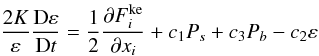 (14c)where we use the form of the flux of ε suggested by Kupka & Mutsham (2007):
  (14d)
(14d)
7. Features of the model: no Ri(cr)
Stably stratified flows are characterized by two competing factors: a shear instability that acts as a source of mixing and a stable temperature gradient that acts as a sink. The two combine into a single parameter, the Richardson number Ri defined in Eq. (13a). The key physical question is whether there is a critical value of Ri beyond which stable stratification overpowers the mixing action of shear so as to lead to zero mixing. The standard RSM models used thus far exhibit a finite critical Richardson number Ri(cr). For example, the Mellor & Yamada model (1982) yields Ri(cr) = 0.19, while the recent model by Cheng et al. (2002) increases the value to Ri(cr) = O(1), thus overcoming the difficulty first raised by Martin (1985) that the MY model yielded too shallow ocean mixed layers. A stability analysis including nonlinearities (Abarbanel et al. 1984) also arrived at Ri(cr) = O(1).
However, even an Ri(cr) ≈ 1 is not satisfactory. In fact, several recent data have shown that mixing persists even after Ri = 1. These data include meteorological observations (Kondo et al. 1978; Bertin et al. 1997; Mahrt & Vickers 2005; Uttal et al. 2002; Poulos et al. 2002; Banta et al. 2002), lab experiments (Strang & Fernando 2001; Rehmann & Koseff 2004; Ohya 2001), LES (Zilitinkevich et al. 2007; Zilitinkevich & Esau 2007), DNS (Stretch et al. 2001), oceanic measurements (Mack & Schoeberlein 2004), and theoretical modeling (Sukoriansky et al. 2005).
Zilitinkevich et al. (2007) constructed a model called “energy and flux-budget turbulence closure” that has no Ri(cr). They then show how the model can explain a wide variety of data. Their model differs significantly from the “main stream” closure models used in traditional second-order closure models. In particular, their parameterization of the pressure-correlations differs from the “standard” ones developed by numerous authors and supported by theoretical and experimental data (Rotta 1951; Launder et al. 1975; Lumley 1978; Zeman & Lumley 1979; André et al. 1978; Mellor & Yamada 1982; Cheng et al. 2002).
Given this situation, Canuto et al. (2008a,b) tried to answer the following question: can the traditional RSM models encompass an arbitrarily large Ri(cr) and what changes are needed to do so without spoiling their documented performance for small and medium Richardson numbers? The answer turned out to be relatively simple since a minimum alteration was required to the previous mixing models to encompass a no-Ri(cr) feature. Specifically, the introduction of the 1 + Ri term in π4 given in Eq. (13i) was all that was needed (such correction does not exist in the unstably stratified case however). Several arguments justifying such an extension were presented in Canuto et al. (2008a), where the performance of the model vs. data is fully discussed.
8. Features of the model: arbitrary Peclet number
In the numerical simulations of Brummel et al. (2002) and Brun & Toomre (2002), Pe is defined as in (13j), but the length scale ℓ is taken to be constant (the depth of the domain), which as we have discussed, is not true near the boundaries. This makes it difficult to compare the results of the numerical simulations in which Pe is taken tobe larger then unity, the smallest value being about 10. As an example, it is difficult to physically interpret Fig. 14 in Brummel et al. (2002) showing that the OV extent decreases as Pe increases. With a constant length scale, the Pe used in such calculations depends only on the rms velocity, and a large Pe corresponds to a large rsm that should entail large rather small OV’s. In the present treatment, Pe is a dynamical variable computed along with all the other variables and not a quantity whose value is assumed.
9. Summary
In many ways, the most surprising aspect of the RSM results is the relative simplicity of the equations determining the Reynolds stresses, heat, and concentration fluxes, since they are linear algebraic equations. This is especially relevant if one considers the amount of information they contain: stable stratification, unstable stratification, rigid rotation, shear, and radiative losses (Peclet number). The two differential equations for K and ε characterize any turbulence model, not this one in particular. We derived the equations that describe mixing in the presence of  (15a)Summarizing our results, we have derived the following equations:

 (15b)
(15b)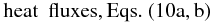

 The model is valid for arbitrary temperature, concentration, and mean velocity gradients, as well as arbitrary Ri and Peclet numbers.
References
- Abarbanel, H. D. I., Holm, D. D., Marsden, J. E., & Ratiu, T. 1984, Phys. Rev. Lett., 52, 2352 [NASA ADS] [CrossRef] [Google Scholar]
- Aller, L. H., & Chapman, S. 1960, ApJ, 132, 1 [Google Scholar]
- André, J. C., DeMoor, G., Lacarrére, P., Therry, G., & du Vachat, R. 1978, J. Atmos. Sci., 35, 1861 [Google Scholar]
- Banta, R. M., Newsom, R. K., Lundquist, J. K., et al. 2002, Boundary-Layer Meteorol., 105, 221 [NASA ADS] [CrossRef] [Google Scholar]
- Bertin, F., Barat, J., & Wilson, R. 1997, Radio Science, 32, 791 [NASA ADS] [CrossRef] [Google Scholar]
- Brummell, N. H., Clune, T. L., & Toomre, J. 2002, ApJ, 570, 825 [Google Scholar]
- Brun, A. S., & Toomre, J. 2002, ApJ, 570, 865 [NASA ADS] [CrossRef] [EDP Sciences] [Google Scholar]
- Canuto, V. M. 1997, ApJ, 482, 827 [Google Scholar]
- Canuto, V. M. 1999, ApJ, 524, 311 (cited as C99) [NASA ADS] [CrossRef] [Google Scholar]
- Canuto, V. M. 2006, Theoretical modeling of Convection. I. Key physical processes, in Convection in Astrophysics, ed. F. Kupka, I. W. Roxburgh, & K. L. V. Chan, 3, Part II, Reynolds Stress Model, IAU Symp., 239, 19 [Google Scholar]
- Canuto, V. M. 2009, Turbulence in astrophysical and geophysical flows, in Interdisciplinary Aspects of Turbulence, Lect. Notes Phys., ed. W. Hillebrandt, & F. Kupka, 107 (Berlin: Springer Verlag) [Google Scholar]
- Canuto, V. M., & Dubovikov, M. S. 1998, ApJ, 493, 834 [Google Scholar]
- Canuto, V. M., Cheng, Y., Howard, A. M., & Esau, I. N. 2008a, J. Atmos. Sci., 65, 2437 [NASA ADS] [CrossRef] [Google Scholar]
- Canuto, V. M., Cheng, Y., & Howard, A. M. 2008b, GRL, 35, L02613 [NASA ADS] [CrossRef] [Google Scholar]
- Chapman, S. 1917, MNRAS, 77, 539 [NASA ADS] [Google Scholar]
- Chapman, S., & Cowling, T. G. 1970, The mathematical theory of non-uniform gases (Cambridge, Univ. Press) [Google Scholar]
- Charbonnel, C., & Talon, S. 2005, Science, 309, 2189 [NASA ADS] [CrossRef] [PubMed] [Google Scholar]
- Charbonnel, C., & Talon, S. 2007, Science, 318, 922 [CrossRef] [PubMed] [Google Scholar]
- Charbonnel, C., & Zahn, J. P. 2007, A&A, 467, L15 [NASA ADS] [CrossRef] [EDP Sciences] [Google Scholar]
- Cheng, Y., Canuto, V. M., & Howard, A. M. 2002, J. Atmos. Sci., 59, 1550 [NASA ADS] [CrossRef] [Google Scholar]
- Favre, A. 1969, in Problems of Hydrodynamics and continuous mechanics, Philadelphia, SIAM, 231 [Google Scholar]
- Kondo, J., Kanechika, O., & Yasuda, N. 1978, J. Atmos. Sci., 35, 1012 [NASA ADS] [CrossRef] [Google Scholar]
- Kupka, F., & Muthsam, H. J. 2007, in Convection in Astrophysics, ed. F. Kupka, I. W. Roxburgh, & K. L. Chan, IAU Symp., 239, 86 (Cambridge Univ. Press) [Google Scholar]
- Landau, L. D., & Lifshitz, E. M. 1987, Fluid Mechanics (New York: Pergamon Press) [Google Scholar]
- Launder, B. E., Reece, G., & Rodi, W. 1975, J. Fluid Mech., 68, 537 [NASA ADS] [CrossRef] [Google Scholar]
- Lumley, J. L. 1978, Adv. Appl. Mech., 18, 123 [Google Scholar]
- Mack, S. A., & Schoeberlein, H. C. 2004, J. Phys. Oceanogr., 34, 736 [NASA ADS] [CrossRef] [Google Scholar]
- Maeder, A., & Meynet, G. 2001, A&A, 373, 555 [NASA ADS] [CrossRef] [EDP Sciences] [Google Scholar]
- Mahrt, L., & Vickers, D. 2005, Boundary-Layer Meteorol., 116, 313 [NASA ADS] [CrossRef] [Google Scholar]
- Martin, P. J. 1985, J. Geophys. Res., 90, 903 [NASA ADS] [CrossRef] [Google Scholar]
- Mathis, S., Palacios, A., & Zahn, J. P. 2004, A&A, 425, 243 [NASA ADS] [CrossRef] [EDP Sciences] [Google Scholar]
- Mellor, G. L., & Yamada, T. 1982, Rev. Geophys. Space Phys., 20, 851 [NASA ADS] [CrossRef] [Google Scholar]
- Michaud, G. 1970, ApJ, 160, 641 [NASA ADS] [CrossRef] [Google Scholar]
- Ohya, Y. 2001, Boundary-Layer Meteorol., 98, 57 [NASA ADS] [CrossRef] [Google Scholar]
- Palacios, A., Talon, S., Charbonnel, C., & Forestini, M. 2003, A&A, 399, 603 [NASA ADS] [CrossRef] [EDP Sciences] [Google Scholar]
- Palacios, A., Charbonnel, C., Talon, S., & Siess, L. 2006, A&A, 453, 261 [NASA ADS] [CrossRef] [EDP Sciences] [Google Scholar]
- Poulos, G. S., Blumen, W., Fritts, D. C., et al. 2002, Bull. Amer. Meteor. Soc., 83, 555 [CrossRef] [Google Scholar]
- Rehmann, C. R., & Koseff, J. R. 2004, Dynamics of Atmospheres and Oceans, 37, 271 [NASA ADS] [CrossRef] [Google Scholar]
- Rotta, J. C. 1951, Z. Physik, 129, 547 [Google Scholar]
- Schatzman, E. 1969, A&A, 3, 331 [NASA ADS] [Google Scholar]
- Strang, E. J., & Fernando, H. J. S. 2001, J. Phys. Ocean., 31, 2026 [Google Scholar]
- Stretch, D. D., Rottman, J. W., Nomura, K. K., & Venayagamoorthy, S. K. 2001, 14th Australasian Fluid Mechanics Conference, Adelaide, Australia, 10–14 December [Google Scholar]
- Sukoriansky, S. B., & Galperin, I. 2005, Phys. Fluids, 17, 1 [CrossRef] [Google Scholar]
- Uttal, T., Curry, J. A., McPhee, M. G., et al. 2002, Bull. American Meteorol. Soc., 83, 255 [NASA ADS] [CrossRef] [Google Scholar]
- Vauclair, S., & Vauclair, G. 1982, ARA&A, 30, 3 [Google Scholar]
- Zeman, O., & Lumley, J. L. 1979, Turbulent Shear Flows (New York: Springer), 1, 295 [Google Scholar]
- Zilitinkevich, S., & Esau, I. 2007, Boundary-Layer Meteorol., 125, 193 [NASA ADS] [CrossRef] [Google Scholar]
- Zilitinkevich, S. S., Elperin, T., Kleeorin, N., & Rogachevskii, I. 2007, Boundary Layer Meteorol., 125, 167 [Google Scholar]
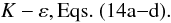
Appendix A: Summary of the model equations
Reynolds stresses: 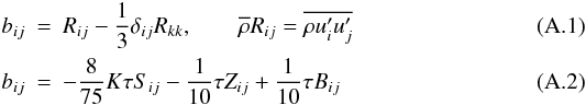
 (A.3)
(A.3) (A.4)
(A.4) (A.5)Heat fluxes,
  :
: ![Mathematical equation: \appendix \setcounter{section}{1} \begin{eqnarray} \label{eq78} (\delta _{ij} + \eta _{ij})J_j^h &=& \gamma _{ij} \beta _j, \quad \beta _i =-\frac{\partial T}{\partial x_i }-\lambda _i \frac{g}{c_p }\\ \label{eq79} \gamma _{ij} &=& \pi _4 \tau (R_{ij} -\pi _2 g\alpha _\mu \tau \lambda _i J_j^\mu ) \nonumber\\ \eta _{ij} &=& \pi _4 \tau \left[S_{ij} +V_{ij} -g\tau \lambda _i (\pi _5 \alpha _T \beta _j +\pi _2 \alpha _\mu \overline \mu _{,j} )\right]. \end{eqnarray}](/articles/aa/full_html/2011/04/aa14447-10/aa14447-10-eq182.png) μ − fluxes,
μ − fluxes,  :
:  (A.8)where:
 ![Mathematical equation: \appendix \setcounter{section}{1} \begin{eqnarray} \label{eq81} d_{ij} &=& \pi _1 \tau (R_{ij} +g\alpha _T \pi _2 \tau \lambda _i J_j^h ) \nonumber\\ \xi _{ij} &=& \pi _1 \tau [S_{ij} +V_{ij} -g\tau \lambda _i (\pi _2 \alpha _T \beta _j +\pi _3 \alpha _\mu \overline \mu _{,j} )]. \end{eqnarray}](/articles/aa/full_html/2011/04/aa14447-10/aa14447-10-eq186.png) (A.9)
(A.9)
Appendix B: Mixing length theory
In the absence of mean velocities and concentration fields, we write the heat flux in the standard form:  (B.1)where the dimensionless Φ represents the ratio of the turbulent diffusivity to the thermometric one. From Eq. (10a) in the 1D case with j = 3, we derive the relation:
  (B.2)Using the relations:
  (B.3)we obtain after some simple algebra (and taking all the coefficients to be of order unity):
 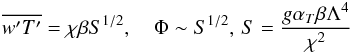 (B.4)which is the well known expression for the heat flux provided by the MLT for the case of efficient convection. In the same limit, we have that the Peclet number is given by:
 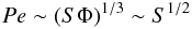 (B.5)
(B.5)
Appendix C: The Ri → ∞ case, analytic solution
Though this version of the model is restrictive, it is of interest to have a complete analytical solution of the problem which we present in what follows. From relations (10a, b) and (12d, e), we obtain that the heat and μ-fluxes are given by the following expressions: ![Mathematical equation: \appendix \setcounter{section}{3} \begin{eqnarray} \label{eq86} J_h &=& \frac{\overline {\rho {w}'{T}'}}{\overline \rho }=K_h \beta , \quad K_h =\tau \overline {w^2} A_h \nonumber\\[-1.5mm] \\ J_\mu &=& \frac{\overline {\rho {w}'{\mu }'}}{\overline \rho} = - K_\mu \frac{\partial \overline \mu}{\partial z},\quad K_\mu =\tau \overline {w^2} A_\mu\nonumber \end{eqnarray}](/articles/aa/full_html/2011/04/aa14447-10/aa14447-10-eq197.png) (C.1)where the dimensionless functions Ah,μ are given by the algebraic relations:
(C.1)where the dimensionless functions Ah,μ are given by the algebraic relations: 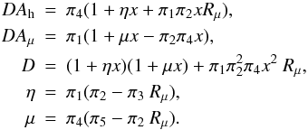 (C.2)The variables π′s are given by relations (13i) and x is defined as follows:
  (C.3)The next step is to solve the Reynolds stress Eqs. (8h). The result is the algebraic relation:
 ![Mathematical equation: \appendix \setcounter{section}{3} \begin{equation} \label{eq89} \overline {\frac{w^2}{2K}} =\left[\frac{30}{7}+ x(A_h -A_\mu R_\mu )\right]^{-1}\cdot \end{equation}](/articles/aa/full_html/2011/04/aa14447-10/aa14447-10-eq203.png) (C.4)The two key variables K-ε still remain to be determined and in principle one has to solve the two differential Eqs. (14a, c). The time scale τ then follows from the definition relation (8i) and all the variables are then known as a function of Ri and Rμ.
(C.4)The two key variables K-ε still remain to be determined and in principle one has to solve the two differential Eqs. (14a, c). The time scale τ then follows from the definition relation (8i) and all the variables are then known as a function of Ri and Rμ.
If a local model can be used, a simplification occurs since Eq. (14a) becomes, after using (7f) and the above results, the following simple expression: 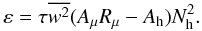 (C.5)Combining (1e) with (C.5), one obtains an algebraic relation only in terms of the variable x which reads:
  (C.6)which, after using relations (1b), can be solved to provide the function:
  (C.7)The explicit form of relation (C.6) upon use of relations (1b), reads as follows:
  (C.8)where:
  (C.9)With the knowledge of x or equivalently τ = 2K / ε, we know the ratio of the variables K-ε but not them singularly. To go further, we adopt a relation of the Kolmogorv type:
  (C.10)where Λ is a mixing length on which we shall comment below. If so, we obtain that the kinetic energy K can now be expressed in terms of the variable x, see relation (C.3), as follows:
 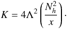 (C.11)If we substitute relation (C.6) into (C.4), we obtain the simple relation:
 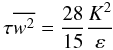 (C.12)and thus the expressions for the heat and μ diffusivities defined in (C.1) take the forms:
 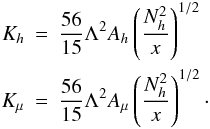 (C.13)Relations (C.13) represent the analytical solution of the turbulent part of the problem. See C99, Figs. 1–16.
The last part of the problem that remains to be solved is the determination of the temperature gradient in the presence of turbulent fluxes which is obtained by solving the flux equation which in simplest form is given by:  (C.14a)where we employ the relations:
  (C.14b)Semi-convectionAs discussed in detail in Paper II, in this case we have ∇ − ∇ad > 0,∇μ > 0,Rμ > 0,
  . Because of the last relation, the solution of Eq. (C.8) must be taken to be negative x < 0 so that relations (C.13) yield a positive diffusivity. Next, if we introduce the dimensionless variable:
 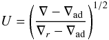 (C.14c)the flux conservation law (C.14a) acquires the form:
 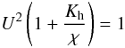 (C.14d)where the ratio
  measures the importance of turbulent diffusivity over the radiative one (we recall that χ has dimensions of cm2 s-1). Using the first of (C.13), we further have that the ratio Kh / χ can be rewritten as:
 ![Mathematical equation: \appendix \setcounter{section}{3} % subequation 2996 4 \begin{eqnarray} \label{eq101} \frac{K_{\rm h}}{\chi} &=& \frac{175}{3\pi ^2}A_h (x)(-x)^{-1/2}\Gamma U,\nonumber\\ \Gamma &=& \frac{8 \pi ^2}{125}\left[\frac{g\Lambda ^4}{\chi ^2H_{\rm p}}(\nabla _r -\nabla _{\rm ad} )\right]^{1/2} \end{eqnarray}](/articles/aa/full_html/2011/04/aa14447-10/aa14447-10-eq232.png) (C.14e)where Γ can be interpreted as an efficiency factor similar to the one in the mixing length scheme (see Appendix B), which can be computed off line. Substituting (C.14e) into (C.14d) yields the following equation for the variable of interest U:
(C.14e)where Γ can be interpreted as an efficiency factor similar to the one in the mixing length scheme (see Appendix B), which can be computed off line. Substituting (C.14e) into (C.14d) yields the following equation for the variable of interest U: 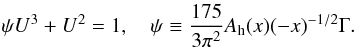 (C.14f)Finally, we note that the Peclet number is defined in Eq. (13j) and enters in the definitions of the π′s given by Eqs. (13i). It is also a function of the variable U since (13j) becomes:
 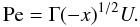 (C.14g)Salt FingersIn this case we have (see Paper II) ∇ − ∇ad < 0, ∇μ < 0, Rμ > 0,
 Thus, x > 0 and relations (C.11), (C.14c) and (C.14g) become:
 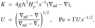 (C.14h)We further have that:
 ![Mathematical equation: \appendix \setcounter{section}{3} % subequation 2996 8 \begin{equation} \label{eq105} \Gamma =\frac{8\pi ^2}{125}\left[\frac{g\Lambda ^4}{\chi ^2H_p }(\nabla _{\rm ad} -\nabla _r )\right]^{1/2}. \end{equation}](/articles/aa/full_html/2011/04/aa14447-10/aa14447-10-eq242.png) (C.14i)The first of Eq. (C.14f) does not change but the variable ψ is now defined as follows:
(C.14i)The first of Eq. (C.14f) does not change but the variable ψ is now defined as follows:  (C.14j)The above relations constitute the analytical solution of the second part of the problem (see C99, Figs. 1–16).
Current usage metrics show cumulative count of Article Views (full-text article views including HTML views, PDF and ePub downloads, according to the available data) and Abstracts Views on Vision4Press platform.
Data correspond to usage on the plateform after 2015. The current usage metrics is available 48-96 hours after online publication and is updated daily on week days.
Initial download of the metrics may take a while.