| Issue |
A&A
Volume 527, March 2011
|
|
|---|---|---|
| Article Number | A107 | |
| Number of page(s) | 10 | |
| Section | Astronomical instrumentation | |
| DOI | https://doi.org/10.1051/0004-6361/201116434 | |
| Published online | 04 February 2011 | |
Revisiting the radio interferometer measurement equation
II. Calibration and direction-dependent effects
Netherlands Institute for Radio Astronomy (ASTRON) PO Box 2,
7990AA
Dwingeloo,
The Netherlands
e-mail: smirnov@astron.nl
Received:
5
November
2010
Accepted:
5
January
2011
Context. Paper I of the series re-derived the radio interferometry measurement equation (RIME) from first principles, and extended the Jones formalism to the full-sky case, incorporating direction-dependent effects (DDEs).
Aims. This paper aims to describe both classical radio interferometric calibration (selfcal and related methods), and the recent developments in the treatment of DDEs, using the RIME-based mathematical framework developed in Paper I. It also aims to demonstrate the ease with which the various effects can be described and understood.
Methods. The first section of this paper uses the RIME formalism to describe self-calibration, both with a full RIME, and with the approximate equations of older software packages, and shows how this is affected by DDEs. The second section gives an overview of real-life DDEs and proposed methods of dealing with them.
Results. A formal RIME-based description and comparison of existing and proposed approaches to the problem of DDEs.
Key words: methods: analytical / methods: numerical / methods: data analysis / techniques: polarimetric / techniques: interferometric
© ESO, 2011
1. Introduction
Paper I of this series (Smirnov 2011a) extended the RIME formalism (Hamaker et al. 1996; Hamaker 2000) to the full-sky case, culminating in the following equation for the visibility matrix measured by interferometer pq:
 (1)The
 term is a 2 × 2
brightness matrix, describing the polarized sky brightness
as a function of direction l,m. The
Gp Jones matrices represent the
per-antenna direction-independent effects (DIEs), which are the provenance of traditional
second-generation calibration (2GC) techniques, most notably selfcal. The
Ep Jones matrices represent the
direction-dependent effects (DDEs).
term is a 2 × 2
brightness matrix, describing the polarized sky brightness
as a function of direction l,m. The
Gp Jones matrices represent the
per-antenna direction-independent effects (DIEs), which are the provenance of traditional
second-generation calibration (2GC) techniques, most notably selfcal. The
Ep Jones matrices represent the
direction-dependent effects (DDEs).
DDEs violate the traditional premise of 2GC, which is that an interferometer array measures
the Fourier transform of one “common” sky. Instead, in the presence of DDEs, each baseline
sees its own apparent sky Bpq. The traditional
premise only holds when the DDEs are identical across all antennas, and
constant in time:
Ep ≡ E.
Under this condition, the apparent sky becomes the same on all baselines:
( ), and
the full-sky RIME becomes simply:
), and
the full-sky RIME becomes simply: 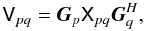 (2)where
 , and the
matrix function
, and the
matrix function  , called the
sky coherency, is the (element-by-element) two-dimensional Fourier
transform of the matrix function Bapp(l,m).
, called the
sky coherency, is the (element-by-element) two-dimensional Fourier
transform of the matrix function Bapp(l,m).
Section 1 of this paper reviews the 2GC calibration problem, and shows how the RIME formalism can be (and has been) applied. Section 2 then looks at the problem of DDEs, describes how they impact calibration, and discusses some current and future approaches.
1. Calibration and the RIME
In the traditional (2GC) view, calibration refers to a process by which the instrumental errors are estimated and corrected for, imaging is the processes of turning the corrected visibilities into an image, followed by deconvolution to take out the effects of the point spread function. While algorithms such as Cotton-Schwab CLEAN (Schwab 1984) have blurred the boundaries between imaging and deconvolution, the separation between calibration and imaging is firmly entrenched in 2GC selfcal implementations (where the two processes are typically implemented via completely separate tools), and has historically led to a divergence of the algorithm development community into “calibration people” and “imaging and deconvolution people”.
The RIME, and recent developments in understanding of DDEs, have been eroding this
distinction. On the one hand, advances in image reconstruction techniques (for an overview,
see Rau et al. 2009) have been usurping some
traditional functions of calibration, while new methods of source modelling on the
calibration side, such as the use of shapelets (Yatawatta et al. 2010, in prep.), rely on
increasingly elaborate models being constructed for a large part of the flux (with
traditional imaging then only used for the lower-level residuals). In RIME terms, both
processes should be thought of as two aspects of the same optimization problem: estimating
 ,
Ep(l,m) and
Gp in an equation such as
(1) that yield the best fit to a set of
observed visibilities (“data”) Dpq. Traditional selfcal solves
for the direction-independent terms
Gp, traditional imaging yields
the , and the
non-trivial DDEs
Ep(l,m) have
(traditionally) been ignored. The historical calibration–imaging separation corresponds to a
two-stage recursive optimization process.
,
Ep(l,m) and
Gp in an equation such as
(1) that yield the best fit to a set of
observed visibilities (“data”) Dpq. Traditional selfcal solves
for the direction-independent terms
Gp, traditional imaging yields
the , and the
non-trivial DDEs
Ep(l,m) have
(traditionally) been ignored. The historical calibration–imaging separation corresponds to a
two-stage recursive optimization process.
1.1. Implicit RIMEs
Existing 2GC packages all make use of some implicit version of the RIME. It is useful to consider at least one example in depth. In Paper III (Smirnov 2011b), I shall be comparing the results of a MeqTrees calibration using an explicit RIME to those obtained with the NEWSTAR package on the same data. NEWSTAR therefore makes for a perfect example.
The exact form of the RIME implemented by NEWSTAR depends on the options used1. The one relevant to the reductions of Paper III is:
 (3)The
constituent parts of this equation are as follows:
(3)The
constituent parts of this equation are as follows:
-
Xspq is the coherency of source s. NEWSTAR sky models are composed of discrete point sources or extended Gaussian components. For a point source,
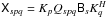 .
. -
Bs is the source brightness. This can be further parameterized in terms of Stokes IQUV, spectral index and rotation measure.
-
Qspq is a per-source correction factor to account for time and bandwidth smearing (see Paper I, Smirnov 2011a, Sect. 5.2).
-
Es is the primary voltage beam gain. NEWSTAR uses an analytic approximation of the WSRT beam (see Sect. 2.1.1). This is implicitly treated as a trivial DDE, i.e. constant in time and the same across all stations.
-
Xpq is thus the “model visibilities”, i.e. the sum of coherencies of all sources in the model.
-
Gp is a diagonal matrix of complex per-station gain terms.
-
Mpq is a 2 × 2 matrix of multiplicative interferometer errors (see Paper I, Smirnov 2011a, Sect. 5.3), and “ ∗ ” is element-by-element multiplication). Here it is on the inside of the equation rather than on the outside as in Eq. (24) of Paper I: this is due to the way NEWSTAR uses “corrected data” in its selfcal procedure.
NEWSTAR’s calibration and imaging procedure typically consists of some combination of and/or iteration over the following steps:
-
Gain calibration: find
 that minimizes
 in a least-squares sense. Compute “corrected data” as
-
Closure errors: find
 that minimizes
 . Compute “corrected data”
as
. Compute “corrected data”
as  (where “ ÷ ” is
element-by-element division – the inverse of “ ∗ ”).
(where “ ÷ ” is
element-by-element division – the inverse of “ ∗ ”). -
Model subtraction: Compute “residual data” as
 .
Rpq thus contains the visibility contribution of
faint background sources not present in the model, corrected for the estimated
antenna gains and interferometer errors.
.
Rpq thus contains the visibility contribution of
faint background sources not present in the model, corrected for the estimated
antenna gains and interferometer errors. -
Imaging and deconvolution: turn the Rpq visibilities into an image, and deconvolve it using Högbom CLEAN.
-
Source finding: Perform a source finding procedure on the residual image to update the sky model.
-
Model update: Solve for the parameters of the new sources by minimizing
 (usually on a small subset of the data).
 -
Model restore: Add the sky model into residual images (after another calibration/subtraction cycle, if the model was updated), using a Gaussian restoring beam.
1.2. Explicit RIMEs
An example of an explicit RIME is implemented in CASA. This also relies on the concept of
model visibilities: 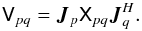 (4)Here,
Xpq is the model visibility (which may be computed from an
image and/or a list of NEWSTAR-like components), and
Jp is composed of several
different Jones terms, typically (Myers et al.
2010, Appendix E.1):
(4)Here,
Xpq is the model visibility (which may be computed from an
image and/or a list of NEWSTAR-like components), and
Jp is composed of several
different Jones terms, typically (Myers et al.
2010, Appendix E.1): 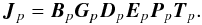 (5)Each term has its own
specific implementation (in case of known terms) and parameterization (in case of solvable
terms). Finally, multiplicative interferometer-based errors
(Mpq) may be optionally applied to either the outside of the
equation (as per Eq. (24) of Paper I, Smirnov
2011a), or to Xpq itself (a-la NEWSTAR, see Eq. (3) above).
(5)Each term has its own
specific implementation (in case of known terms) and parameterization (in case of solvable
terms). Finally, multiplicative interferometer-based errors
(Mpq) may be optionally applied to either the outside of the
equation (as per Eq. (24) of Paper I, Smirnov
2011a), or to Xpq itself (a-la NEWSTAR, see Eq. (3) above).
Conceptually, calibration in CASA is very similar to the procedure described in the previous section, but the use of an explicit RIME confers several advantages. The known terms of the Jones chain (Eq. (5)) can be taken into account properly, while the solvable terms can be solved for in different combinations. The caveats of using such a specific form of the RIME have already been discussed in Paper I (Smirnov 2011a, Sect. 6.2).
Note that although CASA also relies on the essentially 2GC-rooted concepts of model and corrected visibilities, the framework has been successfully used for the development of algorithms for calibration and correction of DDEs, namely W-projection (Cornwell et al. 2008), pointing selfcal (Bhatnagar et al. 2004) and AW-projection (Bhatnagar et al. 2008). I will discuss these further in Sect. 2.
1.3. Phenomenological RIMEs
My experiments with calibration in MeqTrees have favoured phenomenological RIMEs (Noordam & Smirnov 2010). Rather than writing out long Jones chains such as that of Eq. (5), which attempt to follow the physics of the signal propagation chain, the phenomenological approach consists of using a RIME with the minimum number of solvable terms needed to represent the cumulative effect of the chain. Each phenomenological term then ends up subsuming several different physical effects. The rationale for this approach is that, on the one hand, we only need to capture the overall effect for purposes of calibration, while on the other hand, the individual effects often cannot be distinguished at all, apart from their different behaviour in time and frequency – which we try to capture with individual phenomenological terms.
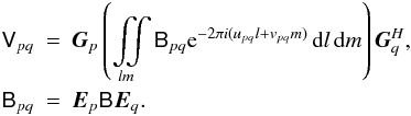
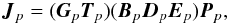
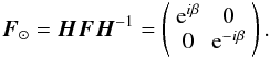
For example, a full-polarization bandpass-gain calibration of the WSRT can be done2 using the following phenomenological RIME:
 Here,
Gp is a solvable diagonal
complex matrix with rapid variation in time, and none in frequency. This subsumes
antenna/receiver gains (G-Jones, in CASA nomenclature) and atmospheric
phase (T-Jones).
Bp is a solvable full 2 × 2
complex matrix with high variability in frequency, but little to none in time. This
subsumes bandpass (B-Jones), polarization leakage
(D-Jones) and on-axis beam gain (E-Jones). More
real-life examples of phenomenological RIMEs will be discussed in Paper III (Smirnov 2011b).
Here,
Gp is a solvable diagonal
complex matrix with rapid variation in time, and none in frequency. This subsumes
antenna/receiver gains (G-Jones, in CASA nomenclature) and atmospheric
phase (T-Jones).
Bp is a solvable full 2 × 2
complex matrix with high variability in frequency, but little to none in time. This
subsumes bandpass (B-Jones), polarization leakage
(D-Jones) and on-axis beam gain (E-Jones). More
real-life examples of phenomenological RIMEs will be discussed in Paper III (Smirnov 2011b).
Where a specific Jones term is known from a priori considerations, it can and should be
inserted into a phenomenological RIME. For example, the equation above would not be
suitable for polarization calibration of the VLA because of parallactic angle rotation.
The equation would need to be rewritten with an extra P-Jones term, which
is not solved for, but rather computed analytically: 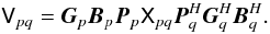 (6)One must be mindful
of matrix (non)commutation when constructing phenomenological RIMEs. The reason the full
CASA Jones chain of Eq. (5) can be captured
by the much simpler Eq. (6) is because some
Jones matrices do commute (see also Paper I, Smirnov 2011a, Sect. 1.6). In particular, T-Jones is
scalar and so commutes with everything, while the CASA B-Jones and
G-Jones are diagonal and so commute among themselves. This allows us to
rewrite Eq. (5) as:
(6)One must be mindful
of matrix (non)commutation when constructing phenomenological RIMEs. The reason the full
CASA Jones chain of Eq. (5) can be captured
by the much simpler Eq. (6) is because some
Jones matrices do commute (see also Paper I, Smirnov 2011a, Sect. 1.6). In particular, T-Jones is
scalar and so commutes with everything, while the CASA B-Jones and
G-Jones are diagonal and so commute among themselves. This allows us to
rewrite Eq. (5) as:
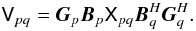
 which makes the link to
Eq. (6) obvious.
which makes the link to
Eq. (6) obvious.
To give a counter-example, in the presence of significant Faraday rotation (time-variable or differential, see Sect. 2.2.2), this equation is not appropriate, because the Faraday rotation term Fp (placed at the right-hand side of the chain) does not commute, and so would necessitate an extra term in Eq. (6).
1.4. The impact of the RIME on calibration
The reasoning used above to construct phenomenological RIMEs illustrates one of the biggest benefits that the RIME formalism has brought to the field of calibration. Pre-RIME, descriptions of signal propagation effects were ad hoc and approximate, while arguments about the order in which they should be calibrated for were difficult to follow. The RIME formalism has recast all this in terms of straightforward and rigorous matrix algebra.
The second benefit of the RIME formalism is the clarity it has brought to polarization calibration. Note that the implicit NEWSTAR RIME given above (Eq. (3)) ignores polarization effects almost completely. NEWSTAR does have some polarization calibration capabilities (as do other 2GC packages), but these are specifically tuned to the WSRT case. The RIME formalism allows for a much more general description of polarization effects. The D and P terms of the CASA RIME (Eq. (5)) are an example, but see also the discussion of differential Faraday rotation in Sect. 2.2.2.
Perhaps most importantly, the RIME gives us the mathematical language to tackle the problem of DDEs, which will be the subject of the next section.
1.5. Calibration ambiguities
No discussion of calibration with the RIME can be complete without mentioning the ambiguity problem pointed out by Hamaker (2000, 2006). In classical selfcal, there is a well-known flux and position ambiguity: multiplying all the antenna gains by a complex factor a, and the source coherency by a-2, does not change the observed visibilities. Therefore, selfcal by itself cannot determine absolute fluxes and positions – these require known calibrators. There is a full-polarization equivalent to this, but it is extremely difficult to formulate and understand outside the RIME formalism.
For a direct analogue, consider a RIME such as that in Eq. (2). For any non-singular matrix A, we have:
 In other words,
we can multiply all the per-antenna uv-Jones terms by A, and
the source coherency by
In other words,
we can multiply all the per-antenna uv-Jones terms by A, and
the source coherency by  and
and  ,
without changing the observed visibilities. Therefore, we need known calibrators to
properly fix the Gp’s. Having
observed a calibrator source, we can fix the brightness
(and therefore the
coherency
,
without changing the observed visibilities. Therefore, we need known calibrators to
properly fix the Gp’s. Having
observed a calibrator source, we can fix the brightness
(and therefore the
coherency  ), and solve for
Gp. However, it is easy to
see that an unpolarized calibrator alone is insufficient. The brightness (and coherency)
matrix of an unpolarized source is scalar, so for any unitary3 matrix U, we have
), and solve for
Gp. However, it is easy to
see that an unpolarized calibrator alone is insufficient. The brightness (and coherency)
matrix of an unpolarized source is scalar, so for any unitary3 matrix U, we have
 , or:
, or:
 Thus, given a
known but unpolarized sky, we can only determine
Gp to within an arbitrary
unitary ambiguity factor U. In other words, we
cannot fix the polarization response of our system without polarized calibrators.
A physical example of such an ambiguity is rotation of all dipoles by the same
angle: this cannot be detected through observations of an unpolarized source.
Thus, given a
known but unpolarized sky, we can only determine
Gp to within an arbitrary
unitary ambiguity factor U. In other words, we
cannot fix the polarization response of our system without polarized calibrators.
A physical example of such an ambiguity is rotation of all dipoles by the same
angle: this cannot be detected through observations of an unpolarized source.
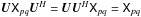
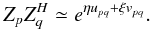
As it turns out, even a polarized calibrator alone is insufficient,
though the matrix algebra gets a bit complicated at this point. The
matrix is
Hermitian positive-definite by construction, and has a Cholesky decomposition4, i.e. there exists a lower-triangular
 such that
 . For any unitary
U, we then have:
. For any unitary
U, we then have:
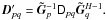
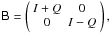
 Therefore, given a
single polarized calibrator, we still have an ambiguity factor of
Therefore, given a
single polarized calibrator, we still have an ambiguity factor of
 !
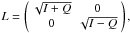
Physical examples of this are somewhat more elaborate, but perhaps the simplest one is
that a source with Q polarization only is insensitive to a certain
combination of dipole rotation and gain adjustment. Indeed, for
!
Physical examples of this are somewhat more elaborate, but perhaps the simplest one is
that a source with Q polarization only is insensitive to a certain
combination of dipole rotation and gain adjustment. Indeed, for
 we have
 and,
given a rotational U, the resulting ambiguity factor is
and,
given a rotational U, the resulting ambiguity factor is
 The upshot of this is
that unambiguous calibration of the polarization response of an interferometer requires
multiple polarized calibrator sources, and/or additional assumptions
about the sky (e.g. V = 0, which was a common assumption in the pre-RIME
era). Hamaker (2006) explores these issues in more
detail.
The upshot of this is
that unambiguous calibration of the polarization response of an interferometer requires
multiple polarized calibrator sources, and/or additional assumptions
about the sky (e.g. V = 0, which was a common assumption in the pre-RIME
era). Hamaker (2006) explores these issues in more
detail.
We should note that though the matrix equations above may seem somewhat complicated, they are far more succinct and complete than any scalar equations that have been used to describe polarization calibration prior to the RIME. Once again, the RIME provides a rigorous mathematical language to describe what is otherwise an extremely tricky problem.
2. Direction-dependent effects (DDEs)
Most of the problems associated with non-trivial DDEs are already pointed to by Eq. (1). The fundamental assumption of traditional selfcal is that DDEs are trivial, meaning that:
-
Each observed visibility Vpq is a measurement of the sky coherency function
 at point
upq, corrupted by some
combination of multiplicative (per-antenna or per-interferometer) gain terms.
at point
upq, corrupted by some
combination of multiplicative (per-antenna or per-interferometer) gain terms. -
The coherency function
is a Fourier transform
of the apparent sky Bapp(l) (see also
Eq. (2)).
DDEs are a multiplication in the lm plane, which corresponds to a
convolution in its Fourier counterpart, the uv plane. That is, in the
presence of non-trivial DDEs
Ep(l)
(including a non-trivial Wp term), the observed
visibility is actually a convolution of the sky coherency. Assuming
Gp ≡ 1 for the moment,
Eq. (1) then gives us: 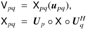 (7)where
“°” is a matrix convolution (i.e. following the same rules as matrix multiplication, with
each elementary multiplication replaced by a convolution), and the convolution kernels
Up are Fourier transforms of
the sky-Jones terms Ep. We can
rewrite this equation to emphasize the time variability, and the fact that any given
interferometer pq only samples one point
upq of the uv
plane at a time:
(7)where
“°” is a matrix convolution (i.e. following the same rules as matrix multiplication, with
each elementary multiplication replaced by a convolution), and the convolution kernels
Up are Fourier transforms of
the sky-Jones terms Ep. We can
rewrite this equation to emphasize the time variability, and the fact that any given
interferometer pq only samples one point
upq of the uv
plane at a time: ), \\ \nonumber \coh{X}{pq}[t] & = & \jones{U}{p}[t] \circ \coh{X}{} \circ \jonesT{U}{q}[t], \\ \nonumber \coh{X}{} & = & {\cal F} \coh{B}{}, \; \jones{U}{p}[t] = {\cal F}\jones{E}{p}[t]. \end{eqnarray}](/articles/aa/full_html/2011/03/aa16434-11/aa16434-11-eq86.png) (8)This
equation captures the heart of the DDE problem: DDEs convolve the “ideal” visibilities, with
(in the general case) a different kernel per every antenna and time sample. Instead of
sampling one uv plane (
(8)This
equation captures the heart of the DDE problem: DDEs convolve the “ideal” visibilities, with
(in the general case) a different kernel per every antenna and time sample. Instead of
sampling one uv plane ( ), we have a separate
uv plane per each pq and time interval
(Xpq[t]), and we’re sampling each such
plane at only one (or at most a handful) of points. Convolution is not uniquely reversible
at the best of times; with such limited sampling it is even less tractable. This is the
reason why in the presence of DDEs, corrected visibilities (in the sense of
Sect. 1.1) do not exist. To be more
precise, they may exist in the mathematical sense, but recovering them is an inverse (and
ill-posed) problem.
), we have a separate
uv plane per each pq and time interval
(Xpq[t]), and we’re sampling each such
plane at only one (or at most a handful) of points. Convolution is not uniquely reversible
at the best of times; with such limited sampling it is even less tractable. This is the
reason why in the presence of DDEs, corrected visibilities (in the sense of
Sect. 1.1) do not exist. To be more
precise, they may exist in the mathematical sense, but recovering them is an inverse (and
ill-posed) problem.
In this section, I will first consider the two common sources of DDEs: the ionosphere and the primary beam, and then discuss some proposed methods of dealing with them.
2.1. E-Jones: beam-related DDEs
The primary beam gain, commonly designated as the E-Jones, is the single
most ubiquitous DDE (since every telescope, after all, has a beamshape of some kind), and
probably the most problematic5. The implicit
simplifying assumption of 2GC packages is that the interferometer observes an “apparent
sky”: that is, some true sky ,
attenuated by a power beam
|E(l,m)|2. Given a reasonably
accurate model for the beam, the final images can be multiplied by
|E(l,m)|-2 to correct the flux scale
(at the cost of increasing the image noise away from centre).
In RIME terms, this classical assumption corresponds to an E-Jones that
is a trivial DDE (i.e. constant in time, and same across all stations), but also the same
for both receivers and thus scalar:
Ep(t,l,m) ≡ E(l,m).
We can then commute the E term in the apparent sky Eq. (1), which becomes a simple multiplication of
the true sky by
EEH = |E|2.
(Incidentally, this also shows why classical selfcal does not concern itself with the
complex phase of the primary beam).
Real-life beams deviate from these assumptions in a number of ways, some of them less well understood than others.
2.1.1. The WSRT and VLA E-Jones
The WSRT primary beam is commonly approximated as:
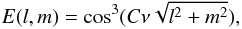 where
C has a very mild dependence on ν (i.e. is
effectively constant for a given band). This model is only valid for the main lobe, down
to about the 10% level. Popping & Braun
(2008) have made a detailed empirical study of the WSRT primary beam, which
shows significant four-fold symmetric structure out in the sidelobes (caused by the feed
legs). More significantly, they have shown a quasi-periodic “ripple” in the off-axis
beam gain as a function of frequency, with a period of ~17 MHz. This is commonly seen
in the observed spectra of off-axis sources.
where
C has a very mild dependence on ν (i.e. is
effectively constant for a given band). This model is only valid for the main lobe, down
to about the 10% level. Popping & Braun
(2008) have made a detailed empirical study of the WSRT primary beam, which
shows significant four-fold symmetric structure out in the sidelobes (caused by the feed
legs). More significantly, they have shown a quasi-periodic “ripple” in the off-axis
beam gain as a function of frequency, with a period of ~17 MHz. This is commonly seen
in the observed spectra of off-axis sources.
Similarly to the WSRT cos3 model, the VLA primary beam has a reasonable analytic approximation using Jinc functions, which is valid to about the 5% level of the main lobe (Uson & Cotton 2008). Brisken (2003) has made electromagnetic simulations that show the sidelobe structure. What significantly complicates the VLA case is beam squint (the beam pattern of the R and L receptors being offset w.r.t. the pointing centre due to the feeds being off-axis), and parallactic angle rotation.
2.1.2. Parallactic angle rotation
An alt-az mount telescope, without a dish derotator such as that designed into ASKAP (Johnston et al. 2008), has an intrinsically time-variable beamshape in the lm frame, as the nominal beam pattern rotates with parallactic angle. Like any DDE, this causes significant spatial artefacts around off-axis sources that cannot be addressed by classical selfcal. This has been a serious dynamic range limitation at the VLA, but some recent developments promise to alleviate the problem. Uson & Cotton (2008) describe a CLEAN-like algorithm (implemented in the Obit package) that corrects these artefacts during deconvolution; the RIME-derived AW-projection method of Bhatnagar et al. (2008) can correct them during imaging. Note that both methods rely on an a priori beam model, and have, to date, been only been applied to VLA data, for which the Brisken simulations provide a very detailed beam model. It remains to be seen whether the more approximate models available for other instruments will prove to be a limiting factor.
The WSRT’s equatorial mounts (and ASKAP’s derotator) keep the beamshape stationary in the lm frame, thus avoiding this problem entirely.
A particularly troublesome situation arises when a sufficiently bright source is located in a sidelobe or near a null, where sky rotation causes rapid variation in the beam gain, and the accuracy of existing beam models is low. Such sources have to be calibrated and subtracted separately, either via some kind of peeling procedure, or by using the differential gain approach described in Sect. 2.4.3. Even at the WSRT, where rotation is not an issue and the beam gain remains (at least in principle) constant in time, sources in a sidelobe need to be treated very carefully, due to the rapid spectral variation caused by the 17 MHz ripple.
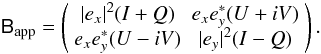
2.1.3. Instrumental polarization
Instrumental polarization comes about due to the beam patterns of the two receptors being non-identical. In RIME terms, this corresponds to E-Jones being diagonal rather than simply scalar:
 which causes an
unpolarized off-axis source to “acquire” some Q (or V,
if using circular receptors):
which causes an
unpolarized off-axis source to “acquire” some Q (or V,
if using circular receptors):
 The WSRT case is rather
simple: the beamshape of each dipole is slightly elongated rather than circularly
symmetric. Since these beamshapes are stationary w.r.t. the sky, the net result is an
“apparent sky” with a non-uniform polarization response:
The WSRT case is rather
simple: the beamshape of each dipole is slightly elongated rather than circularly
symmetric. Since these beamshapes are stationary w.r.t. the sky, the net result is an
“apparent sky” with a non-uniform polarization response:
 Similarly to power beam
attenuation, this effect can be removed (to the extent that the primary beam is known)
via a linear correction to the final images.
Similarly to power beam
attenuation, this effect can be removed (to the extent that the primary beam is known)
via a linear correction to the final images.
For the VLA, non-identical receptor beams are caused by the aforementioned squint; the squint offset rotates with parallactic angle (and thus as a function of time). This leads to a rather complicated picture of instrumental polarization, but is essentially the same problem (with the same solutions) as primary beam rotation.
Note that in contrast to the the WSRT case, the simulations of Brisken (2003) show that the VLA E-Jones has non-trivial elements on the off-diagonal. This is an example of direction-dependent polarization leakage. Leakage has been commonly associated with slight errors in dipole orientation, electromagnetic cross-talk, etc., and treated as a direction-independent effect (Hamaker et al. 1996; Noordam 1996); Brisken’s results demonstrate that it is actually a DDE.
Finally, it should be mentioned that the polarization aberration described by Carozzi & Woan (2009) can also be treated as direction-dependent instrumental polarization (see Paper I, Smirnov 2011a, Sect. 5.4).
The RIME makes it explicit that effects as (variable) primary beam attenuation, instrumental polarization, and leakage, which are treated separately (if at all) in 2GC, can in fact be represented by a single Jones term, and treated via a single mechanism. Perhaps the most stark example of this is provided by aperture array beams, such as those of LOFAR (Yatawatta 2008). With the dipoles of an aperture array fixed on the ground, E(l,m) towards any specific sky direction exhibits complex time-dependent behaviour in all four matrix elements. This completely blends the boundary between primary beams, leakage and instrumental polarization.
2.1.4. Pointing errors and dish deformation
All telescopes mispoint to some extent. This is caused by gravitational load, thermal
expansion, wind pressure, errors in the drive mechanics or even the control software,
etc. In RIME terms, this can be represented by a station-dependent offset in the beam
pattern, causing a nominally identical beamshape E to
produce a different response per station:  (9)The offset
δlp,δmp
is, in general, time-variable. Since the effect of mispointing on observed visibilities
is roughly proportional to
∂E/∂l
and
∂E/∂m,
it is lowest at the centre of the beam (where the beamshape is flat), and highest on the
flank of the beam and around the nulls. Classical selfcal tends to “absorb” the effect
of mispointing in the direction of the dominant source into the per-station amplitude
gain solutions.
(9)The offset
δlp,δmp
is, in general, time-variable. Since the effect of mispointing on observed visibilities
is roughly proportional to
∂E/∂l
and
∂E/∂m,
it is lowest at the centre of the beam (where the beamshape is flat), and highest on the
flank of the beam and around the nulls. Classical selfcal tends to “absorb” the effect
of mispointing in the direction of the dominant source into the per-station amplitude
gain solutions.
Mispointing is thought to be a major source of off-axis errors in WSRT and VLA maps, and thus has been the subject of many studies. Bhatnagar et al. (2004) proposes a modification to the selfcal algorithm called pointing selfcal, which consists of solving for the δlp,δmp parameters during selfcal. This is predicated on having accurate models for both E(l,m) and the off-axis sources, and sufficient SNR to constrain the solution. Pointing selfcal has been shown to work with simulated data, and recently with real VLA observations (Bhatnagar, priv. comm.) Paper III (Smirnov 2011b) will discuss a different approach to the pointing problem.
The environmental factors responsible for mispointing can also cause deformation of the dish surface. The resulting changes to E(l,m) are rather more difficult to predict and quantify, and little work has been done on the subject. Harp et al. (2010) show significant thermal-related deformations at the Allen Telescope Array (ATA).
2.2. Ionosphere and troposphere
The ionosphere becomes a particularly troublesome DDE at low frequencies, owing to the ∝ ν-1 behaviour of ionospheric phase delay, and ∝ ν-2 behaviour of Faraday rotation. For a more detailed look at the ionosphere and its effects on signal propagation, see Thompson et al. (2001, Sect. 13.3) and Intema et al. (2009). Below I will briefly summarize ionospheric effects in terms of the RIME.
2.2.1. Ionospheric phase
Ionospheric phase delay is caused by excess pathlength due to refraction. In the RIME formalism, it corresponds to a scalar Jones term: Zp = eiζp, where ζp ∝ Tν-1, and T is the Total Electron Content along the line-of-sight. Phase delay can easily reach 102−104 rad at lower frequencies, with variations on relatively short timescales and small spatial scales, thus making for a rather severe DDE. Following Lonsdale (2005), we can identify distinct observational regimes based on the size of the array (A), the projected size of the FoV (V), and the scale structure of the ionosphere (S), i.e. the spatial scale on which ionospheric phase is approximately linear. The first criterion is FoV size:
-
Narrow FoV: V ≪ S, making ionospheric phase effectively constant over the FoV (Zp(l) ≡ Zp(0)), and thus a DIE. Since Zp is scalar, it can be commuted to any position in the RIME and absorbed into another Jones term, such as the per-antenna complex gain that is solved for during regular selfcal.
-
Wide FoV: V ≥ S, and therefore Zp is properly direction-dependent.
The second criterion is array size:
-
Tiny array: A ≪ S. Ionospheric phase is constant on scales of A, thus Zp = Zq for all p,q. This makes
 , so the
interferometer does not “see” the ionosphere at all.
, so the
interferometer does not “see” the ionosphere at all. -
Compact array: A ≈ S. Ionospheric phase is approximately linear on scales of A. Crucially, this means that for any direction l and baseline pq, the observed phase difference ζp − ζq is proportional to the projection of the baseline u onto the ionospheric screen, and thus:
 (10)
(10) -
Extended array: A > S. Different stations of the array are looking through completely different parts of the ionosphere.
The tiny array case is trivial and not considered further. Lonsdale regimes 1 and 2 correspond to narrow FoVs with compact or extended arrays: these can be dealt with using regular selfcal. In regime 3 (wide FoV, compact array), the ionosphere manifests itself as an apparent “distortion” of the field: each source is shifted by its own (time-variable) offset η,ξ. This can be easily seen by inserting the Z-Jones given by Eq. (10) into the full-sky RIME of Eq. (1), and merging it with the complex exponent.
Finally, Lonsdale regime 4 corresponds to an extended array and wide FoV. This is the
regime in which MWA and LOFAR are expected to operate.
 then results in a
baseline- and direction-dependent phase offset, which causes each source in the field to
be “smeared” with a different PSF. Selfcal tends to take care of the offset towards the
dominant source, thus producing an image which is adequate in the vicinity of the
dominant source, but gets increasingly distorted away from it.
then results in a
baseline- and direction-dependent phase offset, which causes each source in the field to
be “smeared” with a different PSF. Selfcal tends to take care of the offset towards the
dominant source, thus producing an image which is adequate in the vicinity of the
dominant source, but gets increasingly distorted away from it.
2.2.2. Faraday rotation
Faraday rotation (FR) is rotation of the EM field vector that occurs during propagation
through a medium of free electrons in the presence of a magnetic field. In RIME terms
(and assuming a linear-polarization coordinate basis), the corresponding Jones term is a
rotation matrix: 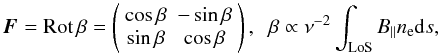 (11)where “LoS”
stands for line-of-sight, B∥ is the component of the
magnetic field parallel to the LoS, and ne is the electron
density. In a circular-polarization coordinate basis (see Paper I, Smirnov 2011a, Sect. 6.3), F becomes a
differential phase delay of the left- and right-polarized components:
(11)where “LoS”
stands for line-of-sight, B∥ is the component of the
magnetic field parallel to the LoS, and ne is the electron
density. In a circular-polarization coordinate basis (see Paper I, Smirnov 2011a, Sect. 6.3), F becomes a
differential phase delay of the left- and right-polarized components:
 The obvious
observational effect of FR is a frequency-dependent rotation of the angle of
polarization. FR associated with the interstellar medium can, for purposes of
calibration, be considered an intrinsic property of the sky per se. Because of the
ν-2 behaviour, ionospheric FR at higher frequencies is
practically negligible. For all these reasons, FR has been an obscure effect, largely
ignored outside of the field of polarimetry.
The obvious
observational effect of FR is a frequency-dependent rotation of the angle of
polarization. FR associated with the interstellar medium can, for purposes of
calibration, be considered an intrinsic property of the sky per se. Because of the
ν-2 behaviour, ionospheric FR at higher frequencies is
practically negligible. For all these reasons, FR has been an obscure effect, largely
ignored outside of the field of polarimetry.
This has changed with the advent of large low-frequency arrays such as LOFAR. In 2010,
the first LOFAR long baseline (Effelsberg-Exloo) detected a strange effect: at certain
frequencies, an unpolarized source was showing significant signal in
the XY/YX correlations, and
practically none in XX/YY (Wucknitz 2010). After considerable excitement, this
was linked to differential FR (DFR). This effect is an excellent
example of the explanatory power of the RIME formalism, so it is worth considering in
some detail. At low frequencies, ionospheric FR can be as high as several cycles (e.g.
15 cycles at 100 MHz, see Thompson et al. 2001,
Sect. 10.3) so the DFR between two stations of a long baseline can reach significant
fractions of a cycle. Consider what happens when an unpolarized 1 Jy point source at
phase centre (Kp ≡ 0) is subject to an FR
of π/2[+2πn] on station
p, and 0[+2πn] on station q.
In the absence of other effects, the measured visibility will be:  (12)or in other words, all
the original I flux will be detected as V! This
clearly shows that DFR is not only a polarimetric concern, but is a mainstream
calibration problem.
(12)or in other words, all
the original I flux will be detected as V! This
clearly shows that DFR is not only a polarimetric concern, but is a mainstream
calibration problem.
Perhaps the most striking feature of Eq. (12) is how it describes a complicated physical effect with very trivial mathematics. This is a great example of the simplicity brought by the 2 × 2 formalism. Interestingly, this very effect was predicted by Hamaker et al. (1996) in the original RIME paper, but (perhaps owing to the relative opacity of the 4 × 4 Mueller formalism, with which it was described) was not immediately recalled when actual DFR was detected6.
2.2.3. Refraction, curvature and absorption
Ionospheric absorption is a relatively small amplitude effect (e.g. 0.1 dB at 100 MHz and ZA = 60°, see Thompson et al. 2001), and is mostly subsumed by the overall gain calibration. Differential absorption makes for a non-trivial DDE, but this is tiny.
Ionospheric refraction causes an apparent shift of position of the source within the primary beam. This can be on the order of 0.05° (at 100 MHz and ZA = 60°). The corresponding change in primary beam gain can be a significant effect, but is probably not in excess of that caused by uncertainties in the primary beam pattern itself. It can therefore be absorbed by whatever primary beam calibration scheme is applied to the data.
Finally, Anderson (priv. comm.) has pointed out that refraction through a curved ionosphere should produce a phase DDE, due to the fact that the apparent baseline (i.e. the baseline as seen by the refracted wavefront) changes. The Anderson effect should be detectable on LOFAR’s long baselines, but it is not yet clear whether it can be separated from Z-Jones per se.
2.2.4. The troposphere
The troposphere adds its own phase delay, with a roughly ∝ ν behaviour. Because most of the effect actually happens very close to the ground, tropospheric phase delay Tp is essentially a Regime 2 effect (i.e. a DIE), and can be subsumed into the overall complex gain calibration7.
Tropospheric refraction can be significant at low elevations (Thompson et al. 2001, Sect 10.1), so telescopes incorporate a pointing correction to account for it. Differential tropospheric refraction (DTR), caused by the curvature of the Earth (i.e. by different antennas “seeing” a source at slightly different elevations) should cause a very small DDE. There are hints of this in high-dynamic-range WSRT data (de Bruyn, priv. comm.), but more work is required to confirm detection of this. Likewise, an analogue of the Anderson effect should also apply to the troposphere, but it is not clear whether this can be detected.
2.3. Correcting for known DDEs
Even when a (non-trivial) DDE is known (whether a priori or from calibration), correcting for it is a non-trivial problem. Several approaches to this have been proposed.
2.3.1. Facet imaging
If a DDE is known (and constant in time), it may be trivially corrected for in a single
direction l0 by applying the inverse of the
Jones term
Ep(l0).
For example, given the observed visibilities in Eq. (1), we can apply correction factors of
 and
and
 . The resulting
visibilities will then be given by:
. The resulting
visibilities will then be given by: 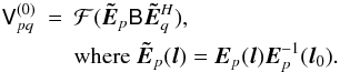 We
can then use standard imaging techniques (i.e. the inverse Fourier transform) to compute
We
can then use standard imaging techniques (i.e. the inverse Fourier transform) to compute
 .
Since
.
Since  with
l → l0, the
resulting image is equal to the “true” sky at
l0 (
with
l → l0, the
resulting image is equal to the “true” sky at
l0 ( ), and diverges from it as
we get away from l0. This is the essence of the
facet (or polyhedron) imaging technique pioneered by
Cotton and Schwab (for an overview, see Cornwell
& Perley 1992). The direction
l0 corresponds to the center of a facet. By
imaging many small facets (each with its own correction factor), and stitching the
resulting images together, we can approximate the “true” sky to arbitrary precision (by
making the facets suitably small). Facet imaging is available in many 2GC packages, and
is well-tested and understood. Its major drawback is the high computing cost (when many
facets are involved), and the fact that time variability in
Ep cannot be taken into
account.
), and diverges from it as
we get away from l0. This is the essence of the
facet (or polyhedron) imaging technique pioneered by
Cotton and Schwab (for an overview, see Cornwell
& Perley 1992). The direction
l0 corresponds to the center of a facet. By
imaging many small facets (each with its own correction factor), and stitching the
resulting images together, we can approximate the “true” sky to arbitrary precision (by
making the facets suitably small). Facet imaging is available in many 2GC packages, and
is well-tested and understood. Its major drawback is the high computing cost (when many
facets are involved), and the fact that time variability in
Ep cannot be taken into
account.
2.3.2. AW-projection
A far more promising alternative is suggested by convolutional function approaches. The first of these was the W-projection algorithm proposed by Cornwell et al. (2008), which corrects for the Wp term on-the-fly during imaging. This is now routinely available in the CASA imager (and also the in lwimager tool of the casarest package, which shares the same codebase). Bhatnagar et al. (2008) have generalized this approach to arbitrary DDEs. The resulting AW-projection algorithm has been tested in an experimental version of CASA, and it is planned to make it available in future releases (Bhatnagar, priv. comm.)
The crucial insight underlying the AW-projection algorithm is that a convolution such
as Eq. (8) can be efficiently computed
both in the forward direction, during the degridding step (when predicting visibilities
from an image), or in the reverse direction, when gridding visibilities for imaging, on
the condition that Up has
limited support (i.e. is significantly non-zero only within a limited area around the
origin), which is the same thing as
Ep being sufficiently
smooth. If we further assume
Ep to be (approximately)
unitary (i.e.  ), then Eq. (8) may even be (approximately) inverted by
computing the convolution
), then Eq. (8) may even be (approximately) inverted by
computing the convolution ![\hbox{$\jonesT{U}{p}[t] \circ \coh{V}{pq} \circ \jones{U}{q}[t]$}](/articles/aa/full_html/2011/03/aa16434-11/aa16434-11-eq164.png) . There is a fixed
computational cost associated with the extra convolution kernels, but it scales to wider
fields a lot more favourably than the facet imaging approach.
. There is a fixed
computational cost associated with the extra convolution kernels, but it scales to wider
fields a lot more favourably than the facet imaging approach.
In other words, AW-projection provides an accurate method to apply known DDEs in the forward direction (i.e. when predicting visibilities from a model image), and an approximate method to correct for them in the reverse direction (when imaging).
While W-projection has been in use for a while and is well-tested, the limitations of the more general AW-projection method are still poorly understood. In particular, it is not clear how (or whether) dynamic range is limited by (a) non-unitarity of Ep, and (b) the fact that high-order terms in Up are ignored (i.e. the limited support assumption). No doubt this understanding will improve as implementations of the algorithm become widely available to the community.
2.3.3. Subtraction in the uv-plane
Given a known sky model, the most straightforward way of dealing with a known DDE is to directly evaluate Eq. (1) in the forward direction, and subtract it from the observed visibilities. This gives us the residuals Rpq = Dpq−Vpq, which can then be corrected for the DIEs. Once imaged, they will still be subject to DDEs on the same relative level. However, if a significant portion of the flux is accounted for by the sky model, then the absolute level of DDE-related artefacts will be much lower, perhaps even below thermal noise (if the sky model is sufficiently deep – and a sufficiently deep model is a requirement for calibration anyway). The sky model itself can be added (“restored”) directly into the residual images with no error. This method was used for the reduction of Paper III (Smirnov 2011b), and produced the “showcase” image of Fig. 1 therein.
For a sky model composed of discrete source components, this is also called the DFT approach, since evaluating Eq. (1) on a per-source basis is equivalent to doing a brute-strength Discrete Fourier Transform. There has been considerable debate in the literature and at meetings about the relative merits of the DFT approach vs. FFT-based methods such as AW-projection. DFTs have the advantage of maximum precision (at least to the extent that the DDE is known), but are very expensive computationally, since they scale linearly with the number of sources being modelled. AW-projection is approximate (see above), but its computational cost scales much better, as it only depends on resolution.
It should be made clear that the two approaches are complementary rather than mutually exclusive, and can be favourably combined (provided compatible implementations are available, which is a matter of some urgency), by using DFTs for the brighter sources in the field, and AW-projection for the fainter ones. By choosing a flux threshold, one can then achieve a clear trade-off between accuracy (and, ultimately, dynamic range) and computational cost.
2.4. Calibrating the unknown DDEs
2.4.1. Selfcal contamination
None of the 2GC packages provide any explicit capabilities for calibration of the
unknown DDEs, since they all assume an implicit RIME similar to Eq. (3), with a single direction-independent gain
term. Consider a very simplified picture, with a field consisting of only two discrete
point sources with brightnesses of B0 and B1, and assume DIEs of
unity. The observed visibilities Dpq are then given by
Eq. (15) of Paper I (Smirnov 2011a), with
Gp ≡ 1: 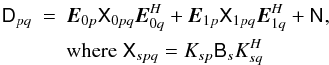 (13)and
 is a 2 × 2
matrix of Gaussian noise. Traditional selfcal (assuming a perfectly known sky model)
then attempts to fit Dpq with the following RIME:
is a 2 × 2
matrix of Gaussian noise. Traditional selfcal (assuming a perfectly known sky model)
then attempts to fit Dpq with the following RIME:
 (14)in
a least-squares sense, over all baselines pq. Obviously, the
best-fitting
(14)in
a least-squares sense, over all baselines pq. Obviously, the
best-fitting  as B1 → 0. On the other hand, if B1 ≃ B0,
 will be some kind of
average between E0p and
E1p. Because of the
complex phase behaviour in the K terms, this is difficult to analyse in
detail. To get a qualitative picture, let us consider the scalar case. Assume that
Ep is scalar and purely
real, and that the sources are unpolarized, so Bs is scalar
as well:
Bs = Is. We
can see that the biggest discrepancies (in amplitude) occur when the phases of the
additive terms in Eq. (13) add either
constructively or destructively. In these two cases, we get:
will be some kind of
average between E0p and
E1p. Because of the
complex phase behaviour in the K terms, this is difficult to analyse in
detail. To get a qualitative picture, let us consider the scalar case. Assume that
Ep is scalar and purely
real, and that the sources are unpolarized, so Bs is scalar
as well:
Bs = Is. We
can see that the biggest discrepancies (in amplitude) occur when the phases of the
additive terms in Eq. (13) add either
constructively or destructively. In these two cases, we get:
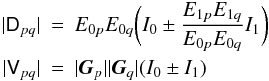 For
any non-trivial array configuration, each baseline has a different fringe rate, so at
any point in time some baselines will be closer to constructive addition, and others
will be close to destructive addition. Therefore, no set of
can achieve a
perfect fit of Dpq to Vpq.
However, from the above we can infer an upper bound on the relative error of the fit:
For
any non-trivial array configuration, each baseline has a different fringe rate, so at
any point in time some baselines will be closer to constructive addition, and others
will be close to destructive addition. Therefore, no set of
can achieve a
perfect fit of Dpq to Vpq.
However, from the above we can infer an upper bound on the relative error of the fit:
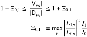 (15)I
shall call Ξ0,1 the selfcal contamination
factor (of source 1 into source 0). I do not have a formal proof for a lower
boundary on the error terms in Eq. (15),
but extensive simulations with MeqTrees suggest that it is also proportional to
Ξ0,1. We can therefore summarize these considerations as
follows: in the presence of DDEs, traditional selfcal will tend to subsume the DDEs in
the direction of the dominant source into its selfcal gain solutions; the fitted
visibilities will be subject to contamination from the unmodelled DDEs
towards the next-brightest source, with a relative error proportional to
Ξ0,1.
(15)I
shall call Ξ0,1 the selfcal contamination
factor (of source 1 into source 0). I do not have a formal proof for a lower
boundary on the error terms in Eq. (15),
but extensive simulations with MeqTrees suggest that it is also proportional to
Ξ0,1. We can therefore summarize these considerations as
follows: in the presence of DDEs, traditional selfcal will tend to subsume the DDEs in
the direction of the dominant source into its selfcal gain solutions; the fitted
visibilities will be subject to contamination from the unmodelled DDEs
towards the next-brightest source, with a relative error proportional to
Ξ0,1.
Similar considerations apply to any discrepancies (i.e. missing sources, etc.) in the sky model. Ultimately, selfcal contamination makes itself felt via artefacts in the resulting images, which can be extraordinarily complicated and counter-intuitive (for an example, see Fig. 17 of Paper III, Smirnov 2011b).
2.4.2. Peeling
The peeling algorithm was originally proposed by Noordam (2004) as a way of calibrating and removing DDEs from bright sources one by one, in order of decreasing brightness. Since its introduction, the term “peeling” has been misunderstood and diluted to the point where it is occasionally used to describe any technique incorporating direction-dependent solutions, but this is incorrect. In its original formulation, peeling refers to a very specific calibration algorithm:
-
1.
A normal selfcal solution is performed, using an equation suchas (3). The resulting
solutions will
tend to incorporate DDEs in the direction of the brightest source
s0. - 2.
The prediction for s0 is subtracted from the data. This is the “peeling” step per se: our best estimate for the visibility contribution of s0 is, in a sense, peeled away.
-
3.
Optionally, the
 visibilities are corrected by applying
  .
.
-
4.
Optionally, the
visibilities are phase-shifted to the position of the next-brightest source
s1 and averaged down in time and frequency (to smear
out the contribution of other sources). -
5.
The
visibilities are presumably dominated by source s1. We
now go back and repeat the procedure for s1.
Peeling has the considerable advantage that all existing 2GC calibration packages provide sufficient functionality to implement its steps, so it has been widely tested and accepted in the community.
The major drawback of peeling is that it can be very expensive computationally. Note that the solutions at step 1 are subject to selfcal contamination Ξs0,s1. This error is “frozen in” at step 2, when the fitted visibilities (for source s0) are subtracted from the data. It can then further contaminate the solutions for s1 (in addition to the contamination Ξs1,s2. If the source being peeled is truly dominant, then this contamination can be negligible, but if the brightness of s0 and s1 is comparable, it can become pretty severe. These errors can be driven down by repeated iterations through the peeling cycle (with clever subtraction of sources), at the cost of significant CPU and I/O overhead. This makes peeling impractical when dealing with more than just a few sources.
2.4.3. Differential gains
The differential gains approach is closely related to peeling. It may
be thought of as a generalized, simultaneous form of peeling. A detailed practical
example will be discussed in Paper III (Smirnov
2011b), but the essence is to use a RIME of the form: 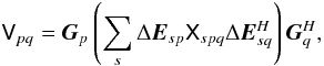 (16)and solve for
Gp on small time/frequency
scales (as per normal selfcal), then simultaneously solve for
ΔEps on larger
time/frequency scales, for a subset of fainter sources. The
Gp solutions then subsume
all DDEs in the direction of the dominant source, while the
ΔEps terms account for the
difference towards the fainter sources. If some of the DDEs are known
a priori, suitable terms for them can be inserted into the equation above in addition to
ΔEps. The differential
gain solution will then account only for the remaining unknown DDEs.
(16)and solve for
Gp on small time/frequency
scales (as per normal selfcal), then simultaneously solve for
ΔEps on larger
time/frequency scales, for a subset of fainter sources. The
Gp solutions then subsume
all DDEs in the direction of the dominant source, while the
ΔEps terms account for the
difference towards the fainter sources. If some of the DDEs are known
a priori, suitable terms for them can be inserted into the equation above in addition to
ΔEps. The differential
gain solution will then account only for the remaining unknown DDEs.
Note that solving for ΔE on a single off-axis source is equivalent to peeling the dominant source and solving for the off-axis source (with suitable solution intervals chosen for each selfcal step). The ΔE approach overcomes a lot of the drawbacks of peeling (contamination of solutions and frozen-in errors, the need for repeated selfcal cycles) by doing a single simultaneous solution in one step.
Differential gains share a common weakness with peeling: that of proliferation of degrees of freedom (DoF’s). This is partially mitigated by using larger solution intervals, but it is obvious that we cannot simultaneously solve for ΔEps towards all sources in a typical field, since that would be gross over-fitting. (Not to mention the CPU cost of solving for that many parameters simultaneously, which would probably become prohibitive first.)
2.4.4. Parametrized models and beacon sources
The DoF issue can be addressed if the DDE in question can be represented by a parametrized model for Ep. We can then solve for the parameters of that model (presumably, few in number), and then correct for the resulting Ep estimate using one of the methods of Sect. 2.3.
A number of approaches have shown that this is feasible. For the ionosphere, the field-based calibration (FBC) method of Cotton et al. (2004) uses the position offsets of sources (in individual snapshot images) to fit a global phase screen over the array. The source peeling and atmospheric modelling (SPAM) algorithm of Intema et al. (2009) does a similar fit to phase solutions obtained via peeling (in AIPS). Both methods show how to work around the limitations of 2GC packages: since direct fits to visibilities are impossible in the framework of the latter, especially without a fully-fledged RIME, they rely on standard calibration methods (including peeling), and fit a model to the results of calibration. Hull et al. (2010) have demonstrated a similar approach for E-Jones, using source fluxes to fit the FWHM parameter of the ATA beam.
Given an explicit RIME, it should be possible to fit parametrized models directly to the observed visibilities. The minimum ionospheric model (MIM) approach proposed by Noordam is similar to FBC and SPAM, in that it purports to fit a smooth model for ionospheric phase, but is different in that it uses visibilities (but also other sources of data, such as GPS measurements). This requires a software system where explicit RIMEs may be implemented, and so cannot be adapted to 2GC packages, but it has been demonstrated in the LOFAR BBS system, using a simple linear-slope MIM. The pointing selfcal method (Bhatnagar et al. 2004) already mentioned above is an application of the same approach to pointing errors.
All these methods have the common feature of relying on beacon sources, that is, having enough sources in the field to constrain the solutions. The availability of a sufficient number of beacons is a crucial question for the calibratability of future instruments. I will return to this in the conclusion to Paper III (Smirnov 2011b), after the results presented therein have been considered.
Note that, just as in the DFT-vs.-FFT debate discussed in Sect. 2.3.3, there is a related dichotomy between the parametrized model approach, and methods based on direction-dependent solutions (peeling, differential gains). The latter methods require the use of DFTs at the predict stage, since the FFT approach (AW-projection) cannot be applied without a model of Ep(l) for the entire field. Parametrized models, on the other hand, may be applied both via DFT and FFT.
Once again, I suggest that the two approaches should be treated as complementary. Looking ahead, the results of Paper III (Smirnov 2011b) will show that brighter off-axis sources exhibit all sorts of complicated structure in their ΔEp solutions, even in the relatively uncomplicated (i.e. low-DDE) case of WSRT 21 cm observations. It is hard to see how this can be captured by a parametrized DDE model to a precision sufficient for error-free subtraction of such sources. This suggests a similar trade-off in accuracy vs. computing cost as that described in Sect. 2.3.3, leading to the following hybrid approach for dealing with DDEs:
-
1.
The unknown DDEs are calibrated for via parametrizedmodel(s), which [hopefully] accounts for the bulk of the effect.
- 2.
In addition, ΔEp solutions are obtained for the brighter off-axis sources, to account for any deviations from the sky or DDE models towards those sources.
- 3.
The brightest sources are predicted and subtracted via DFT.
- 4.
Fainter sources are predicted and subtracted via FFT.
- 5.
The residuals are corrected for during imaging using AW-projection.
Note that the sets of sources involved at steps 2, 3 and 4 are conceptually similar to “Cat I” and “Cat II” sources proposed for LOFAR calibration (Nijboer & Noordam 2007), but here I suggest three sets rather than two. The exact partitioning of sources into sets determines the accuracy vs. computing cost trade-off.
2.4.5. Comparative summary of approaches
It may be interesting to compare the different approaches to a particular class of DDE, for instance pointing error. Pointing errors introduce an E-Jones as given by Eq. (9). To date, three relevant approaches have been proposed: pointing selfcal (Bhatnagar et al. 2004), peeling (Sect. 2.4.2) and differential gains (Sect. 2.4.3). Of these, peeling is by far the best tested, since it is available with all 2GC software packages. Differential gains are available in MeqTrees; pointing selfcal is implemented in an experimental version of CASA (Bhatnagar, priv. comm.), but is not publicly available at time of writing. This makes a quantitative comparison impossible, but the algorithms may be compared in principle.
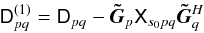
The peeling approach and differential gains are very similar in that they attempt to solve for the same phenomenological effect: a direction-dependent complex gain term. In essence, peeling approximates a full-sky RIME as:
 where
Xspq is the model coherency of source s
(typically a phase-shifted delta function, for a point source model, but Gaussian
sources are also possible in e.g. NEWSTAR). Peeling consists of a least-squares solution
for for one set of gains at a time (as in regular selfcal), followed by “temporary”
subtraction of sources for which a solution has been obtained. Differential gains uses
an equation like (16). First, a regular
selfcal step is done to obtain
Gp solutions on short
time/frequency scales. This is followed by a simultaneous least-squares solution for all
the
ΔEsp
terms, on longer time/frequency scales.
where
Xspq is the model coherency of source s
(typically a phase-shifted delta function, for a point source model, but Gaussian
sources are also possible in e.g. NEWSTAR). Peeling consists of a least-squares solution
for for one set of gains at a time (as in regular selfcal), followed by “temporary”
subtraction of sources for which a solution has been obtained. Differential gains uses
an equation like (16). First, a regular
selfcal step is done to obtain
Gp solutions on short
time/frequency scales. This is followed by a simultaneous least-squares solution for all
the
ΔEsp
terms, on longer time/frequency scales.
Peeling is subject to selfcal contamination at each stage of the process, due to the as-yet-unsolved-for contributions of fainter sources. This is especially severe when sources have comparable flux. Differential gains overcomes this by solving for all sources simultaneously. In principle, it should be possible to drive contamination arbitrarily low (and thus achieve the same result as differential gains) via several iterations of the peeling cycle, but this is both labour-intensive, and requires many passes through the data.
Both approaches solve for per-antenna, per-direction gains, while overlooking the fact
that physically, these are due to a single per-antenna pointing offset (and thus
ignoring Eq. (9)). Pointing selfcal
tries to solve for the true offset itself. In effect, it uses a RIME of the form of
Eq. (7), where the convolutional terms
Up = ℱEp
are the aperture illumination patterns, i.e. the Fourier transforms of the primary beams
Ep, and
are the full-sky
model coherencies. At the heart of the algorithm is a clever minimization scheme, which
essentially decomposes Up into
first- and second-order terms of the pointing offsets
δlp,δmp.
This assumes that the primary beam has a functional form, and that it is (at least to
zero-th order) Gaussian.
The advantage of pointing selfcal is that a single per-antenna pointing offset is obtained, and that the entire model sky (including extended emission!), rather than discrete components, is used to constrain the solution. Peeling and differential gains solve for the total effective gain in each direction, and are less well-constrained by definition. On the other hand, the latter two approaches will happily absorb all unknown DDEs into the direction-dependent solution, while it is yet unclear to what extent pointing selfcal is robust in the presence of other DDEs. The fact that the entire sky is used to constrain the solution also seems to be a double-edged sword. In particular, it is not clear how pointing selfcal is affected by having a bright source near a null or a sidelobe, where the primary beam is particularly poorly approximated by the functional form.
In terms of performance, pointing selfcal should in principle be the fastest method of the three, since it solves for the least number of unknowns, and also allows for the entire sky to be predicted via an FFT. Differential gains are slower, which is partly due to the use of DFTs for source prediction, although the true bottleneck is the far larger number of unknowns. Peeling, on the other hand, is I/O-bound due to the large number of data passes, which will usually make it the slowest of the lot.
3. Conclusions
Several authors have developed approaches to the DDE problem based on the RIME, using different (but mathematically equivalent) versions of the formalism. This paper has attempted to reformulate these using one consistent 2 × 2 formalism, and consider how these methods may be combined.
A look at such DDEs as instrumental polarization (Sect. 2.1) and differential Faraday rotation (Sect. 2.2.2) suggests that the study of polarized signals is no longer a side issue of interest only to polarimetry per se. Proper calibration of the new crop of instruments requires that a full-polarization picture be considered from the beginning. Fortunately, the RIME provides just such a picture, by recasting the signal in terms of 2 × 2 coherency matrices rather than IQUV vectors. This allows complicated propagation effects to be described in terms of rigorous and straightforward matrix algebra, and builds valuable links between one’s physical and mathematical intuition.
The version of the NEWSTAR RIME covered here does not include bandpass or polarization calibration. These options are available in NEWSTAR, but they were not used for the calibration described in Paper III (Smirnov 2011b).
A Hermitian matrix is positive-definite if for all non-zero complex vectors . That is positive-definite follows from Sylvester’s criterion (Gilbert 1991), because and . In fact, the Cholesky decomposition for can be worked out directly:
In the general formulations above, I used E to refer to all DDEs in the signal path. At the risk of confusion, this section will also use E for the beam-related Jones term in particular. The ubiquitous nature of beamshapes, and the problems associated with them, is perhaps a justification for using “E” as the “representative” DDE letter.
According to James Anderson (priv. comm.), the VLBI community was aware of the implications of DFR during the 1970s, and this was a major reason for choosing circularly polarized receptors. Recall that in the circular polarization frame, DFR (or indeed any geometric rotation) becomes a simple phase effect, and can be subsumed into the overall phase calibration. I haven’t been able to locate a citation for this. There are other compelling reasons for using circular receptors in VLBI: parallactic rotation being easier to deal with is one of them.
References
- Bhatnagar, S., Cornwell, T. J., & Golap, K. 2004, EVLA Memo 84. Solving for the antenna based pointing errors, Tech. Rep., NRAO [Google Scholar]
- Bhatnagar, S., Cornwell, T. J., Golap, K., & Uson, J. M. 2008, A&A, 487, 419 [NASA ADS] [CrossRef] [EDP Sciences] [Google Scholar]
- Brisken, W. 2003, EVLA Memo 58. Using Grasp8 To Study The VLA Beam, Tech. Rep., NRAO [Google Scholar]
- Carozzi, T. D., & Woan, G. 2009, MNRAS, 395, 1558 [NASA ADS] [CrossRef] [Google Scholar]
- Cornwell, T. J., & Perley, R. A. 1992, A&A, 261, 353 [NASA ADS] [Google Scholar]
- Cornwell, T. J., Golap, K., & Bhatnagar, S. 2008, IEEE J. Selected Topics in Signal Process., 2, 647 [NASA ADS] [CrossRef] [Google Scholar]
- Cotton, W. D., Condon, J. J., Perley, R. A., et al. 2004, in Ground-based Telescopes, ed. J. M. Oschmann, Jr., SPIE Conf. Ser., 5489, 180 [Google Scholar]
- Gilbert, G. T. 1991, Amer. Math. Monthly, 98, 44 [Google Scholar]
- Hamaker, J. P. 2000, A&AS, 143, 515 [NASA ADS] [CrossRef] [EDP Sciences] [Google Scholar]
- Hamaker, J. P. 2006, A&A, 456, 395 [NASA ADS] [CrossRef] [EDP Sciences] [Google Scholar]
- Hamaker, J. P., Bregman, J. D., & Sault, R. J. 1996, A&AS, 117, 137 [NASA ADS] [CrossRef] [EDP Sciences] [Google Scholar]
- Harp, G., Meitzner, S., & Croft, S. 2010, in SKA Calibration and Imaging Workshop 2010 [Google Scholar]
- Hull, C., Bower, G., Kroft, S., et al. 2010, PASP, 122, 1510 [NASA ADS] [CrossRef] [Google Scholar]
- Intema, H. T., van der Tol, S., Cotton, W. D., et al. 2009, A&A, 501, 1185 [NASA ADS] [CrossRef] [EDP Sciences] [Google Scholar]
- Johnston, S., Taylor, R., Bailes, M., et al. 2008, Experim. Astron., 22, 151 [NASA ADS] [CrossRef] [Google Scholar]
- Lonsdale, C. J. 2005, in From Clark Lake to the Long Wavelength Array: Bill Erickson’s Radio Science, ed. N. Kassim, M. Perez, W. Junor, & P. Henning, ASP Conf. Ser., 345, 399 [Google Scholar]
- Myers, S. T., Ott, J., & Elias, N. 2010, CASA Synthesis & Single Dish Reduction Cookbook, Release 3.0.1 [Google Scholar]
- Nijboer, R. J., & Noordam, J. E. 2007, in Astronomical Data Analysis Software and Systems XVI, ed. R. A. Shaw, F. Hill, & D. J. Bell, PASPC, 376, 237 [Google Scholar]
- Noordam, J. E. 1996, The Measurement Equation of a Generic Radio Telescope, Tech. Rep., AIPS++ Note 185 [Google Scholar]
- Noordam, J. E. 2004, in Ground-based Telescopes, ed. J. M. Oschmann, Jr., SPIE Conf. Ser., 5489, 817 [Google Scholar]
- Noordam, J. E., & Smirnov, O. M. 2010, A&A, 524, A61 [NASA ADS] [CrossRef] [EDP Sciences] [Google Scholar]
- Popping, A., & Braun, R. 2008, A&A, 479, 903 [NASA ADS] [CrossRef] [EDP Sciences] [Google Scholar]
- Rau, U., Bhatnagar, S., Voronkov, M. A., & Cornwell, T. J. 2009, IEEE Proc., 97, 1472 [Google Scholar]
- Schwab, F. R. 1984, AJ, 89, 1076 [NASA ADS] [CrossRef] [Google Scholar]
- Smirnov, O. M. 2011a, A&A, 527, A106 [NASA ADS] [CrossRef] [EDP Sciences] [Google Scholar]
- Smirnov, O. M. 2011b, A&A, 527, A108 [NASA ADS] [CrossRef] [EDP Sciences] [Google Scholar]
- Thompson, A. R., Moran, J. M., & Swenson, Jr., G. W. 2001, Interferometry and Synthesis in Radio Astronomy, 2nd edn. (New York: Wiley) [Google Scholar]
- Uson, J. M., & Cotton, W. D. 2008, A&A, 486, 647 [NASA ADS] [CrossRef] [EDP Sciences] [Google Scholar]
- Wucknitz, O. 2010, in ISKAF2010 Science Meeting [Google Scholar]
- Yatawatta, S. 2008, LOFAR-ASTRON Memo 255. LOFAR beamshapes and their use in calibration and imaging, Tech. Rep., ASTRON [Google Scholar]
Current usage metrics show cumulative count of Article Views (full-text article views including HTML views, PDF and ePub downloads, according to the available data) and Abstracts Views on Vision4Press platform.
Data correspond to usage on the plateform after 2015. The current usage metrics is available 48-96 hours after online publication and is updated daily on week days.
Initial download of the metrics may take a while.