| Issue |
A&A
Volume 527, March 2011
|
|
|---|---|---|
| Article Number | A117 | |
| Number of page(s) | 14 | |
| Section | Extragalactic astronomy | |
| DOI | https://doi.org/10.1051/0004-6361/201016138 | |
| Published online | 04 February 2011 | |
A LABOCA survey of submillimeter galaxies behind galaxy clusters
Onsala Space ObservatoryDepartment of Earth and Space Sciences, Chalmers
University of Technology,
439 92
Onsala,
Sweden
e-mail: daniel.p.johansson@chalmers.se
Received: 13 November 2010
Accepted: 24 December 2010
Context. Submillimeter galaxies are a population of dusty star-forming galaxies at high redshift. Measuring their properties will help relate them to other types of galaxies, both at high and low redshift. This is needed in order to understand the formation and evolution of galaxies.
Aims. The aim is to use gravitational lensing by galaxy clusters to probe the faint and abundant submillimeter galaxy population down to a lower flux density level than what can be achieved in blank-field observations.
Methods. We use the LABOCA bolometer camera on the APEX telescope to observe five clusters of galaxies at a wavelength of 870 μm. The final maps have an angular resolution of 27.5″ and a point source noise level of 1.2–2.2 mJy. We model the mass distribution in the clusters as superpositions of spherical NFW halos and derive magnification maps that we use to calculate intrinsic flux densities as well as area-weighted number counts. We also use the positions of Spitzer MIPS 24 μm sources in four of the fields for a stacking analysis.
Results. We detected 37 submm sources, out of which 14 have not been previously reported. One source has a sub-mJy intrinsic flux density. The derived number counts are consistent with previous results, after correction for gravitational magnification and completeness levels. The stacking analysis reveals an intrinsic 870 μm signal of 390 ± 27 μJy at 14.5σ significance. We study the S24 μm–S870 μm relation by stacking on subsamples of the 24 μm sources and find a linear relation at S24 μm < 300 μJy, followed by a flattening at higher 24 μm flux densities. The signal from the significantly detected sources in the maps accounts for 13% of the Extragalactic Background Light discovered by COBE, and the stacked signal accounts for 11%.
Key words: galaxies: clusters: general / submillimeter: galaxies / infrared: galaxies / cosmology: observations
© ESO, 2011
1. Introduction
Submillimeter galaxies form a population of high-redshift, dusty star-forming galaxies that are highly obscured in the visible and in the near-infrared, and have a spectral energy distribution (SED) that peaks in the submillimeter (submm) waveband (see e.g. Blain et al. 2002, for a review). Most recent searches for submm galaxies have been based on surveys of blank sky with no known large-scale structure along the line-of-sight. These surveys have exploited large-format sensitive bolometer arrays (e.g. SCUBA on the James Clerk Maxwell Telescope (JCMT), Coppin et al. 2006; LABOCA on the Atacama Pathfinder EXperiment (APEX), Weiß et al. 2009; AzTEC on ASTE: Austermann et al. 2010; Scott et al. 2010; the South Pole Telescope (SPT): Vieira et al. 2010; MAMBO on the IRAM 30 m telescope: Greve et al. 2004; Bertoldi et al. 2007). Those maps cover large areas at a nearly uniform noise level, leading to a simple selection function with a constant completeness across the field. The observations showed that source number counts increase steeply with decreasing flux density at mm and submm wavelengths (e.g. Weiß et al. 2009; Patanchon et al. 2009). In order to probe the faint (below a few mJy) population of submm galaxies, several authors have taken advantage of the gravitational magnification induced by massive clusters of galaxies (e.g. Smail et al. 1997, 2002; Chapman et al. 2002b; Knudsen et al. 2005, 2006, 2008; Johansson et al. 2010; Wardlow et al. 2010; Rex et al. 2009; Egami et al. 2010). A large magnification, produced for example when a source lies close to a critical line of the lens, may make it possible to detect a source with an intrinsic flux density much lower than the formal root mean square of the noise of the observation. This is the only method of detecting such dim sources directly. Cluster field observations have sensitivities that vary across the map, as magnified sources are “lifted” above the detection limit, and the selection functions are therefore more complicated. The most comprehensive study to date of submm galaxies behind lensing clusters is that of Knudsen et al. (2008), who analyzed SCUBA data from 12 galaxy clusters and one blank field, resulting in an effective surveyed area of 71.5 arcmin2 on the sky, but an area in the source plane almost twice as small. Seven sources with sub-mJy fluxes were detected.
Observed cluster fields.
The sources revealed by gravitational lensing are prime targets for observations across the electromagnetic spectrum. Swinbank et al. (2010) discovered a very bright submm source, situated at z = 2.33, with flux density S870 μm ~ 106 mJy, and molecular line observations showed that the amount of molecular gas is similar to that in local ultra-luminous infra-red galaxies (ULIRGs, Danielson et al. 2010). The z ~ 3.4 submm source studied by Ikarashi et al. (2010) and discovered through use of AzTEC at 1.1 mm (Wilson et al. 2008a) has a 880 μm flux density measured by the Submillimeter Array (SMA) of ~73 mJy and seems to be a ULIRG as well. On the other hand, the z = 2.79 galaxy behind the Bullet Cluster (Gonzalez et al. 2010), with a flux density of about 48 mJy at 870 μm, is more representative of the normal galaxy population with an intrinsic far-infrared luminosity of a few times 1011 L⊙ (Wilson et al. 2008b; Gonzalez et al. 2009; Johansson et al. 2010). Large surveys in the mm (SPT) and the far-infrared (Herschel) are discovering bright lensed submm galaxies (Vieira et al. 2010; Negrello et al. 2010).
Another way to probe the faint part of the submm galaxy population is to perform a stacking analysis using known positions obtained from complementary observations at another wavelength. Dole et al. (2006) used the positions of sources detected with Spitzer Space Telescope at 24 μm to measure the contribution of those sources to the 70 and 160 μm far-infrared background, gaining up to one order of magnitude in depth. Greve et al. (2010) carried out a stacking analysis of the LABOCA submm map of the extended Chandra deep field (ECDF) using a large sample of near-infrared detected galaxies.
In this paper, we extend the analysis of submm sources behind the Bullet Cluster recently presented in Johansson et al. (2010) by four additional galaxy cluster fields observed with the LABOCA receiver on the APEX telescope. The deep observations allow us to detect submm galaxies with observed flux densities above ~4.5 mJy, while the gravitational magnification reveals galaxies with intrinsically fainter flux densities. We derive the magnification of the foreground clusters by using the lens equation for clusters modeled as a superposition of Navarro, Frenk and White (NFW, 1997) mass density profiles whose parameters are inferred from published papers on the selected clusters. From the magnification maps, we calculate intrinsic flux densities and derive submm number counts for the entire survey. We carry out a stacking analysis on 24 μm detected sources in the fields to probe the correlation between submm and mid-infrared emission and detect stacked 870 μm observed flux densities of S870 μm < 800 μJy for sources that are undetected individually in the maps.
This paper is organized as follows: in Sect. 2 we describe the submm observations and data reduction and the Spitzer MIPS 24 μm archival data; in Sect. 3 we present the resulting maps. In Sect. 4 we discuss the lensing models and the number counts and in Sect. 5 we present a stacking analysis. Section 6 discusses the contribution of our submm signals to the Extragalactic Background Light discovered by COBE. The results are summarized in Sect. 7.
Throughout the paper, we adopt the following cosmological parameters: a Hubble constant H0 = 71 km s-1 Mpc-1, a matter density parameter Ω0 = 0.27, and a dark energy density parameter ΩΛ0 = 0.73. The redshift z = 0.3 where three of our clusters reside corresponds to an angular-diameter distance of 911 Mpc and a scale of 4.42 kpc/arcsec. z = 2.2, the median redshift of known submm galaxies, corresponds to an angular-diameter distance of 1728 Mpc and a scale of 8.38 kpc/arcsec1.
2. Observations and data reduction
We have gathered data from galaxy cluster fields observed with the LABOCA bolometer camera on the APEX2 telescope in Chile (Güsten et al. 2006). The five clusters clusters are merging systems, and their high masses yield areas of large gravitational magnification, which increases the possibility of finding intrinsically dim submillimeter sources lensed by the cluster. Three of the cluster field observations are from our own observing programs, while the AC 114 data (Principal Investigators S. Chapman and F. Boone) were downloaded from the ESO archive and the Abell 2163 data were provided by the PI. M. Nord. Detailed information about the cluster fields, including integration time and noise levels of the final maps, is given in Table 1.
Ground-based submm observations suffer from the fact that the Earth’s atmosphere is by far brighter than the astronomical sources. The changing temperature of the atmosphere further complicates the data reduction. The relatively small field-of-view of LABOCA (11.4′) limits the influence of the spatial temperature structure of the atmosphere on the measurement.
LABOCA observes in total power scanning mode, where the telescope scans the sky in a pattern that is designed to facilitate the retrieval of the astronomical signal and the removal of the atmospheric signal. The scanning pattern that was used for our observations is an outwards winding spiral which is repeated at four raster points. At a given time during the scan, the atmospheric signal is correlated across the entire array and we can model and remove it. The faint astronomical signal is not correlated, unless it is distributed on scales comparable to the field-of-view of the bolometer camera. The Minicrush software (Kovács 2008), that we use to reduce the data, utilizes this approach when removing the correlated atmospheric noise.
Several types of calibration data are taken during the observations. Absolute flux calibration is determined from observations of the primary calibrators: Neptune, Uranus and Mars. When no primary calibrator is available, secondary calibrators, which are well studied objects for which the flux ratios to the primary calibrators are known, can be used. Measuring the calibrators also gives a measure of the opacity of the atmosphere. The opacity is also measured by performing skydips, which are fast scans that measure the sky temperature as a function of elevation at constant azimuthal angle. These scans are performed every two to three hours. The calibration of LABOCA data is described in detail by Siringo et al. (2009). The telescope pointing was checked regularly with scans on nearby bright sources and was found to be stable within 3″ (rms). The angular resolution (FWHM) of LABOCA on APEX is 19.5″.
2.1. Data reduction
The data were reduced using the Minicrush software (Kovács 2008), similarly to the procedure described in Johansson et al. (2010). We summarize the steps here. The data are organized in MBFITS-files, where data from each bolometer as a function of time are saved in a so-called timestream. Each scan, and thereby each MBFITS-file, contains the timestream data of half bolometers. Minicrush attempts to remove the correlated noise by temporarily regarding it as a signal, and fitting a model to all the timestreams at the same time. This model is then removed from each timestream, and the result is a cleaner signal, with less correlated noise. This procedure is repeated a number of times (for LABOCA usually six to eight times) until the resulting signal is “white”, that is that most of the 1/f-type noise has been removed.
An advantage of this method for removing correlated noise is that the gains of each individual bolometer can be estimated during the process. Another method for determining the gains is to observe a bright calibration source and scan it to produce a fully sampled map with each bolometer. The information about the gains is used to flatfield the data. It can also be used to flag and remove suspicious bolometer channels from the reduction. A channel with almost no optical response will appear to have very low noise level, but searching for and flagging channels with low gain would find and remove that channel from the reduction. The pipeline also flags spikes and glitches in the bolometer channels.
We used the option “–deep” in Minicrush. This turns on the most aggressive filtering and is useful when searching for point-like sources. Extended structures, such as the Sunyaev-Zeldovich increment from the clusters, are filtered out.
2.2. Making maps
When the pipeline has removed the correlated noise from the atmosphere and from the instrument, flagged optically dead channels and bad pixels (for example hit by cosmic rays), the timestreams should be “white”, i.e. free from 1/f-type noise. The astronomical signal is typically too weak to be seen in the timestreams, and maps from individual scans have to be produced and co-added to reduce the noise. The maps are made by using the scanning pattern of the telescope and map each bolometer position onto a grid of points; when a bolometer has “seen” a certain pixel on the map, its flux is deposited there. Since several bolometers have seen the same portion of the sky, the final flux value in one map pixel is an average of the flux of the bolometers that observed that part of the sky, weighted by the variance of the individual bolometers. A noisy bolometer thus contributes less to the flux density value in a single pixel in the map than a less noisy one.
Together with the flux density map (the “signal” map), a noise map is created. The coadded values of the time stream weights are used to create the noise map. A signal-to-noise map, which is the signal map divided by the noise map, is also appended to the FITS-file.
2.3. Spitzer MIPS data reduction
In Sect. 5 we discuss a stacking analysis in the LABOCA maps on Spitzer MIPS (Rieke et al. 2004) 24 μm source positions. We describe here the MIPS data reduction and source extraction procedure. We follow the general recommendation not to use the pipeline-processed MIPS mosaics, but to re-process the data, because persistent images can create artefacts on the mosaics. Since we use only the 24 μm MIPS data, “MIPS” will refer to that band in the remainder of this paper.
Four of the clusters in our survey have been observed in the 24 μm MIPS band. We used all the available 24 μm data for each cluster field, as summarized in Table 2. We started by downloading the basic calibrated data from the Spitzer science archive. For each astronomical observation request (AOR), we created a flatfield frame using the script “flatfield_24_ediscs.nl”. That frame was then used to correct for any persistent problem in the data. We then used Mopex to do overlap correction on all the data for each target. The overlap-corrected data were then mosaiced using Mopex. We used the default values for all the steps in the pipeline.
Source extraction from the mosaics was performed with the Apex tool. We did point response function (PRF) fitting and aperture photometry to detect significant MIPS sources. The number of detected sources per field is listed in Table 2, together with the MIPS coverage across the LABOCA map, the median noise level for point sources and the 24 μm source number density. For the Bullet Cluster and MS 1054-03, the MIPS maps cover almost the entire LABOCA field, but for AC 114 and Abell 2744 the MIPS map are significantly smaller.
Summary of archival MIPS data used in this study.
 |
Fig. 1 Signal-to-noise maps of the five cluster fields. White circles represent the significant sources in the map and black contours show the noise maps of each cluster map at levels of 2, 4 and 8 mJy beam-1. The signal-to-noise representation causes the appearance of the increasing noise towards the edge of each map to be suppressed. |
3. Results
Figure 1 shows the final reduced signal-to-noise maps of the cluster fields. They have been smoothed with a Gaussian of the size of the beam (19.5″) to a final resolution of 27.5″, and emission on scales larger than 100″ has been filtered out. Contours of the noise maps are overlaid on the signal-to-noise maps.
In the remainder of this section we discuss the source extraction process, and describe the source catalog and the Monte Carlo simulations that we used to characterize the noise level and completeness in each field. We also discuss the method we used for flux deboosting and how we estimated the number of spurious detections.
3.1. Source extraction
Flux densities and magnification factors for submm sources detected in the survey.
We impose a detection threshold of > 3.5σ in the signal-to-noise maps for source extraction. We exclude sources that lie on the edge of the maps where the signal-to-noise representation is not accurate.
In each map we extract any source position with significance > 3.5σ and fit a circular, two-dimensional Gaussian to the same position in the signal map. We limit the size of the Gaussian to that of the beam’s FWHM of the images, because submm galaxies are very likely to be point-like with respect to the LABOCA beam. Tacconi et al. (2006) found a median source-sizes of < 0.5″, derived from interferometric CO line emission observations, in a sample of submm galaxies. In two cases we fit elliptical Gaussians, where we know from previous observations that the LABOCA sources are comprised of emission from two or more galaxies. The two sources are (1) the brightest source in the Bullet cluster (SMM J065837.6-555705), which is known to be a blend of two images of the same z = 2.79 galaxy (see e.g. Wilson et al. 2008b; Johansson et al. 2010; Gonzalez et al. 2010), strongly lensed by the cluster potential and an elliptical cluster member; (2) SMM J105656.4-033622 in MS 1054-03 which has three SCUBA 850 μm counterparts as reported by Knudsen et al. (2008), and is discussed further in Appendix A.
We measure the noise level for each source from the Monte Carlo simulated maps described in the next section. The procedure ensures that neither confusion noise nor nearby sources contaminate the noise estimate.
The final source list is displayed in Table 3. There, we list, together with positions and measured flux densities of each source, deboosted flux densities and gravitational magnification values, which are discussed in the following sections.
3.2. Survey completeness and depth
Monte Carlo simulations are used to analyze the noise levels of the observations and to simulate the completeness of the survey. We create so-called jack-knife maps3, which are the result of coadding all the scanmaps on one target when multiplying half of the scans with − 1. This effectively removes any astronomical emission from the resulting maps, and makes them representations of the instrumental noise only. By randomizing the positive and negative scans a large number of different jackknives can be created, all of which being random realizations of the noise in our observations. For each cluster field we created 500 jack-knife maps.
We note that the confusion noise in the real maps is effectively removed from the jack-knifed maps. This implies that the noise level is underestimated. One can show that at the depth of our maps, the instrumental noise exceeds the confusion noise. To estimate the confusion level, i.e. the flux level where a larger integration time will not decrease the noise level due to the unresolved background sources, we use the standard estimate that confusion occurs when there is one source per 30 beams (Condon 1974; Hogg 2001). We can estimate the confusion level from the relations presented by Knudsen et al. (2008). They used a power law distribution for the number counts (N(>S) = N0S − α, with N0 = 13 000 deg-2 and α = 2.0) of submm galaxies (Barger et al. 1999; Borys et al. 2003). The confusion noise level is then Sconf = (30ΩbeamN0μ1 − α)1/α where μ is the mean gravitational magnification across the field. Thus, the confusion level is lowered by the lensing, and for the map FWHMs of 27.5″ and a mean magnification factor of 1.5, the confusion level is < 3 mJy, which is lower than the faintest detected source in our survey, at 4.6 mJy. The confusion noise is thus much smaller than the instrumental noise, and can be safely neglected in the following analysis.
Noise levels
The jack-knifed maps are used to estimate the noise levels of each map as a function of angular distance from the center. In a circle of increasing size we extract all pixels in each jack-knife map, measure the standard deviation, and then take the average of the values for all the jack-knife maps. This procedure is repeated for increasing values of the radial coordinate. The histograms of the distribution of pixel values in the jack-knife maps are well described by Gaussians, whose standard deviations are measures of the noise level in each cluster map. In Fig. 2 we show the results of that analysis for the five cluster fields. It can be seen that the noise level changes very little out to a radius of 5′. The noise level reached at that distance is the value that we report for each map in Table 1. Also, because the noise level is almost constant in this region, it is the part of the map that we use in the number counts.
From the jack-knives we also estimate the noise level for each detected source. Around the position of the submm source (which is not present in the jack-knife maps) we extract a circular area the size of the beam, and measure the standard deviation for those pixels in each jack-knife map. The average value is reported as the uncertainty in the second column in Table 3.
 |
Fig. 2 Pixel-to-pixel root-mean-square (rms) as a function of radial distance from the map center for the five cluster fields, described in Sect. 3.2. |
Completeness
We simulate the effects of completeness by inserting artificial sources (Gaussians of the size of the LABOCA beam) into randomly chosen jack-knife maps, running the source extraction algorithm, and then comparing the detected sources to the inserted ones. We limit the angular area to the central 10′. Similar analysis have previously been performed by Beelen et al. (2008); Knudsen et al. (2008); Weiß et al. (2009); Johansson et al. (2010). We simulate sources of flux densities from 1 to 15 mJy, increasing incrementally by 0.5 mJy, and make 500 simulations per flux density bin. Although the jackknife maps are realizations of the noise in the maps, it is possible (and consistent with the underlying Gaussian statistics) to find fake “sources” which are noise peaks. We therefore include the condition that a detected source should be situated sufficiently close (within a beam) of the input source.
The results for the completeness simulations of the five LABOCA maps are displayed in Fig. 3. The completeness curves follow the general expected behavior; a noisier map has a lower completeness value at a certain flux density. From the curves we see that for example the Bullet Cluster map is ~70% complete at 4.2 mJy (the 3.5σ limit for source extraction), while for MS 1054-03 at the corresponding flux density of 5.4 mJy the map is 65% complete. At a flux density of 6 mJy the maps are 48% (Abell 2163), 93% (Bullet Cluster), 58% (Abell 2744), 96% (AC 114) and 77% (MS 1054-03) complete.
The completeness curves are used to evaluate the submm number counts. With the 3.5σ significance limit for source extraction we must take undetected sources into account when constructing the number counts, which are discussed in Sect. 4.1.
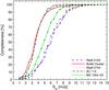 |
Fig. 3 Completeness of the five cluster fields as a function of flux density, as described in Sect. 3.2. |
3.3. Flux deboosting
The faint population of submm sources acts to boost the flux density of the detected sources in the survey. We have used a Bayesian recipe (Coppin et al. 2005) to correct for this flux boosting (see e.g. Scott et al. 2008; Hogg & Turner 1998). The procedure is described in detail in Appendix A of Johansson et al. (2010). A prior flux distribution is calculated in a Monte Carlo simulation, where we create sky maps with sources distributed in flux according to a Schechter distribution, and source positions are drawn randomly, ignoring the effects of clustering4. We generate 106 simulated maps, and calculate a mean flux distribution from the histogram of pixel values for each map. This histogram is our prior flux distribution. The prior is multiplied with the probability of measuring a flux density Sm when the intrinsic flux density is Si. This probability is modeled as a Gaussian distribution, with the observed flux and noise levels in Col. 2 of Table 3 as mean and dispersion. The product of the prior flux distribution and the probability to measure a flux Sm when the intrinsic flux is Si is normalized to yield the posterior flux distribution5. The deboosted flux density corresponds to the x-axis value found at the local maximum of the posterior flux distribution. These values are listed in Table 3. Due to the monotonic decrease of the prior flux distribution, the process yields non-symmetric flux density uncertainties, but as noted in Table 3, the difference between the upper and lower uncertainty is smaller than the number of given digits in the table.
We model the prior distribution by a Schechter function with the following form  (1)(Schechter 1976) with parameters from the SHADES survey (Coppin et al. 2006), that have been scaled from 850 μm to 870 μm using a submm spectral index of 2.7. That yields the following parameter values: N′ = 1703 deg-2 mJy-1, S′ = 3.1 mJy and α = − 2.0.
3.4. Spurious detections
Our adopted criterion for source extraction (S/N ≥ 3.5) means that we are detecting sources close to the noise in the maps. It is therefore possible that some of our detections are spurious; they might be due to a noise peak boosted by confusion noise or instrumental artefacts. It is important to investigate how many of the sources in our catalog might be spurious detections. We do that by employing two different techniques:
-
1.
The number of negative 3.5σ peaks in the maps: we run the sourcedetection algorithm on inverted maps with the same3.5σ criterion, to estimate the number of spurious detections. In the five inverted maps we find four sources, indicating that at least four of the sources in our catalog could be spurious detections.
-
2.
The probability that a source has a negative deboosted flux density: the deboosting algorithm gives us the posterior flux density for each flux/noise-pair, which is a probability distribution for the flux density. For the 37 sources in the survey, we find four that have a ≥ 5% probability of having a negative flux density, and are possibly spurious. These four sources include SMM J161541.2-060817 and SMM J065915.6-560108 which are discussed in the notes of Table 3.
The two methods of estimating the false detections agree well. We note that these calculations only gives a statistical measure of the number of spurious sources, and not which those sources are. However, it is more likely that the least significant sources are false detections.
4. Cluster lens models and number counts
Details about the cluster mass models
The clusters in our survey were partly chosen for their lensing properties because their high masses lead to areas of high magnification. In order to estimate the magnification of the detected sources, knowledge of the mass distribution of the clusters is required. The following calculations use the thin lens approximation.
The magnification factor due to a gravitational lens is given by the relation  (2)where
  is the Jacobian of the lens equation,
 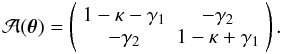 (3)κ is the convergence of the lens while γ1 and γ2 are the components of the complex shear.
We model the clusters as a superposition of one or more spherically symmetric Navarro, Frenk & White (NFW) mass profiles (Navarro et al. 1997). For an NFW profile, the convergence is (Takada & Jain 2003)  (4)and the shear is
  (5)where the critical surface mass density
  (6)where DL is the angular-diameter distance to the lens, DS the distance to the source, and DLS the distance between the source and the lens, and F, G and f are functions of the concentration parameter which can be found in Appendix B in Takada & Jain (2003).
The virial radius of the mass distribution, rvir can be calculated from the virial mass 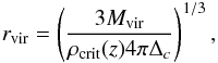 (7)where
 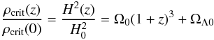 (8)is the critical density at the redshift of the lens in a flat Universe. The virial overdensity Δc can be estimated from a fit to numerical simulations (Bryan & Norman 1998):
 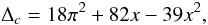 (9)where x = ωm(z) − 1 and
  .
.
We estimate the concentration parameter c for a certain mass and redshift using a fit to X-ray luminous clusters of galaxies (Ettori et al. 2010)  (10)with M ∗ = 1.0 × 10¹⁵ M⊙ and the fitted parameters A = 0.558 ± 0.008 and B = − 0.451 ± 0.023. The resulting magnification factors and number counts do not depend strongly on the assumed c − M relation; using the relation from Bullock et al. (2001) results in magnification factors that differ from those derived from the Ettori et al. (2010) fit at a level lower than the statistical uncertainties.
We wrote a computer program that generates magnification maps by solving Eq. (2) on a two-dimensional grid. Each cluster was modeled as one or a sum of NFW halos, whose masses were taken from mass models in the literature. The parameters for these mass models are summarized in Table 4. We do not include any individual galaxies in our models. We assume the background sources (the source plane) are at a redshift of z = 2.5 but find that the magnifications are not particularly sensitive to changes in source redshift6. By creating magnification maps for the cluster fields, the magnifications of the detected sources could be read out from their position in the maps.
A short discussion of each of the five cluster models follows:
-
Abell 2163: we used the mass from a weaklensing analysis performed by Radovichet al. (2008) and modeled thecluster as a single NFW profile. Work by Maurogordatoet al. (2008) suggests that thecluster is an ongoing merger and that the mass distribution iselongated, which we do not account for in our simple model.
-
1E 0657-56 is the most massive cluster in the survey and gives the largest area with high magnification of the five clusters. It consists of two components, one main cluster and a smaller subcluster. Clowe et al. (2004) fitted the main cluster to a NFW profile and measured the mass of the subcluster using aperture densitometry (Clowe et al. 2000; Fahlman et al. 1994).
-
Abell 2744 is made up of two subclusters aligned along the line-of-sight (Boschin et al. 2006). The subclusters have a mass ratio of 3:1 as estimated from a fit to NFW profiles by Boschin et al. (2006). We use their mass estimate as masses for two concentric NFW profiles.
-
AC 114: we use the results from Campusano et al. (2001) for our model. They improved upon a previous lensing model by Natarajan et al. (1998). Their model of AC 114 is made out of a central cluster component, two smaller subclusters and a galaxy-scale component centered on each bright cluster galaxy. We include the three large components but not the galaxy-scale components in our model.
-
MS 1054-03 consists of three distinct mass concentrations. We model the cluster as three NFW profiles with masses estimated from a fit of three singular isothermal sphere profiles performed by Hoekstra et al. (2000).
The resulting magnification maps are displayed in Fig. 4. The positions of the detected sources for each cluster are overlaid. The magnification values are listed in Table 3, as well as the demagnified flux densities. In Fig. 5 we show the square root of the area (in the image plane) that has a certain magnification factor or larger. This figure shows the complex interplay between mass and redshift that determines whether there are areas of high magnification. Abell 2163, which is the second most massive cluster, is a less effective lens than AC 114 because it is at lower redshift and therefore its mass is distributed over a larger area on the sky.
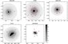 |
Fig. 4 Magnification maps for the five clusters. The positions of the detected submm sources are marked on the maps with circles. |
4.1. Number counts analysis
Since gravitational lensing affects both the observed flux density of a source and the area surveyed, we have to make corrections when calculating number counts. The observed flux of the sources must be demagnified to estimate the intrinsic flux. The intrinsic flux of a source is related to the observed flux by Sobs = μSi where μ is the magnification of the source. Also, because the magnification is not constant across the maps, neither is the sensitivity.
We consider the central 10′ of the maps where the noise is approximately constant (see Fig. 2 and the discussion in Sect. 3.2). We then impose the same significance criterion as for the submm maps: that a source must have a signal-to-noise ratio of 3.5 or higher in order to be reliably detected. This signal-to-noise ratio corresponds to a certain minimum observed flux density Smin. A source with intrinsic flux density of Si is then only detected if it lies in a region with magnification μ ≥ Smin/Si.
The area of this region in the lens plane, Aeff,l( > S), is the effective area that we are surveying for sources of a certain intrinsic flux density or greater. The area in the lens plane corresponds to a smaller area in the source plane due to magnification and the effective area we are surveying in the source plane is  (11)where An is the area in the lens plane of a single area element and μn is the magnification of that particular element. In our case An corresponds to the area of one pixel and μn the magnification of that pixel. Thus a single detected source corresponds to number count of 1/Aeff,s( > S) sources per unit area.
We also account for the effects of incompleteness in the maps, using the Monte Carlo simulations described in Sect. 3.2. For each source we detect with a flux density corresponding to a completeness of C we expect there to be on average Nund = 1/C − 1 undetected sources with the same observed flux density.
By assuming that those undetected sources are uniformly distributed in the map we can calculate the probability that they have a certain intrinsic flux. This probability is  (12)where Aobs → int is the area in the image plane which has a magnification in the interval required to place a source with an observed flux density Sobs into the bin corresponding to Sint. Afield is the total image plane area of the field in which the source lies.
4.2. Resulting number counts
The resulting number counts are shown in Fig. 6, together with the results from the surveys of Beelen et al. (2008) and Weiß et al. (2009) carried out with LABOCA at 870 μm as well as those from SCUBA surveys of Coppin et al. (2006) and Knudsen et al. (2008) at 850 μm, for which the flux values were scaled from 850 μm to 870 μm with a spectral index of 2.7. There is generally good agreement with previous results. A much larger survey of lensing clusters would be needed to reduce the uncertainties and make more secure prediction about the dim submm galaxies. Uncertainties for the number counts were calculated from Poisson statistics, using the tables in Gehrels (1986). The number counts and their uncertainties are presented in Table 5.
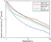 |
Fig. 5 Square-root of the area with magnification > μ as function of magnification (μ) for the five cluster models in the sample. |
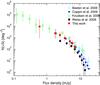 |
Fig. 6 Derived number counts for the survey (filled boxes) compared with results from previous observations. |
5. Stacking analysis
We now turn to the analysis of the undetected sources in the maps. It is well known that the most numerous contribution to the submm galaxy population comes from dim sources with low flux densities (see for example the number counts in Fig. 6). Those dim sources cannot be identified individually in the submm maps, but their presence can be inferred statistically.
Stacking (coadding different parts of a map to lower the noise) has proven to be an efficient method to reveal the underlying dim population of submm sources. Such analysis has been performed by e.g. Scott et al. (2008); Dunne et al. (2009); Greve et al. (2010). Except for Abell 2163, all fields in our sample have available Spitzer MIPS 24 μm data, as summarized in Sect. 2.3.
The MIPS catalogs give us positions and flux densities of all 24 μm sources in the fields, which we use to stack data in our LABOCA maps. We excluded MIPS positions which are farther than 6′ away from the LABOCA map center, where the noise level is rapidly increasing (see Fig. 2). Including positions further out in the map would not lower the noise in the stacked signal. We also excluded MIPS positions that lie closer than the size of the LABOCA beam from the cataloged submm sources in Table 3. For each 24 μm position we extract submaps of size 2′ × 2′ from the LABOCA map (labelled Si). We also extract the same region from the noise map (σi), and use the following relation to stack the submaps:  (13)i.e. a summation weighted by the variance. Lastly, we note that, although no cataloged submm sources will enter the central position of the stacked signal because those positions are discarded, they may contaminate the outskirts of the stacked map. Therefore, we also subtracted models of the cataloged submm sources from the LABOCA maps before stacking. This lowers the noise levels in each of the stacked maps but leaves the stacked flux densities unchanged.
Number counts.
 |
Fig. 7 Stacked 870 μm maps (in units of mJy beam-1) on the 24 μm positions for the cluster fields with MIPS observations, overlaid with signal-to-noise contours. The white contours range between 3σ and 13σ with an increment of 2σ, while the black countours show the − 3σ level. The maps have not been corrected for gravitational magnification. The fifth map is the coadded signal of the four individual stacked maps, which yields a 14.5σ-detection. In Table 6 we present fits to the stacked maps. |
In Fig. 7 we show the stacked images for the four clusters. Each of the stacked maps shows a significant detection in the central region, which is well fitted by a circular Gaussian of the size of the beam. Flux densities and noise levels for the maps are summarized in Table 6. The noise levels of the stacked maps are measured by subtracting the best-fit Gaussians and calculating the pixel-to-pixel rms of the residual maps. The flux densities of the stacked signals range from ~350−820 μJy. This is equal to the mean observed flux density of the sources that contribute to the stacked signal. In general terms, a deeper MIPS catalog yields a lower 870 μm flux value (comparing the stacked fluxes with the 24 μm depth the deeper maps have a lower stacked signal). See also the following section.
The stacked signal corresponds to an observed 870 μm flux density. To investigate the intrinsic fluxes of the dim galaxies we use the magnification maps derived from the cluster models. We find the magnification factor for each 24 μm position in the map and then stack the submaps extracted from the LABOCA map again, this time dividing each submap by the magnification of the central source. This calculation is only valid for the central part of the stacked map, since the magnification is not constant across the submaps. We fit a circular Gaussian to the stacked signals, and report the measurements in the fifth column of Table 6. The demagnified stacked fluxes are lower than the original.
Finally, we coadd the four stacked signals, weighted by their noise-maps, to find the total stacked 24 μm signal for the entire survey (excluding Abell 2163). The map, shown in the fifth panel in Fig. 7, is a 14.5σ-detection, as reported in Table 6. When performing the same operation on the stacked maps corrected for gravitational magnification, we find a mean signal of 390 μJy for the four cluster fields. What would be the properties of an submm galaxy with such a flux density? Assuming a median redshift of z = 2.2 (Chapman et al. 2005), dust temperature Td ~ 40 K and dust emissivity index α = 2, the 870 μm flux density of 390 μJy corresponds to a far-infrared luminosity LFIR ~ 6.4 × 10¹¹ L⊙ (Eq. (11) in De Breuck et al. 2003). By assuming that the submm emission originates mainly from starburst phenomena, which follows a Salpeter initial mass function with a low-mass cutoff ml = 1.6 M⊙, we can estimate a star-formation rate SFR ~ 60 M⊙ yr-1 using Eq. (4) of Omont et al. (2001). It is clear that the stacking analysis uncovers a population of submm sources different from that detected directly in the maps. The derived far-infrared luminosity and star-formation rate depend on several assumptions about the underlying submm population.
Several groups have obtained similar results when stacking on MIPS or radio source positions. Scott et al. (2008) found a stacked signal of 324 ± 25 μJy on ~2000 MIPS positions in the AzTEC study of the COSMOS field (Scoville et al. 2007). Their MIPS map had a similar depth to those in the present study. Accounting for the wavelength difference by scaling the AzTEC 1.1 mm flux density with a mm/submm spectral index of 2–3, the 870 μm flux density would be ~520–660 μJy. This is slightly higher than the intrinsic LABOCA flux density, 390 μJy. Greve et al. (2010) found similar stacked flux values in their study of the Extended Chandra Deep Field South.
5.1. On the validity of the stacking detections
In order to assess the validity of the detection, we perform the stacking analysis on random positions in the LABOCA map, drawn from a uniform distribution within the same map area as the 24 μm maps. We run 20 such simulations for each field. None of the simulated maps has stacked signal with a significant 870 μm source in the center. The nondetection in the simulated maps gives confidence in the stacking results on the real 24 μm position, and shows a correlation between the MIPS and LABOCA maps. We discuss the nature of this correlation in more detail in the next section.
Results from the stacking analysis.
 |
Fig. 8 Top panel: normalized histogram of the signal-to-noise values in the LABOCA maps at the 24 μm positions (dash-dotted line), compared with the mean histogram from 20 sets of random positions (solid line). Lower panel: difference signal between the signal-to-noise histogram above, showing that the main part of the stacked signal is due to sources with signal-to-noise ratios between 0.5 and 2. This histogram clearly shows a deficit of points at negative signal-to-noise units and an excess at positive signal-to-noise units. |
To investigate the significance of the sources that contribute to the stacked signals, we extract pixel values at the 24 μm positions from the signal-to-noise maps and compare them to the randomly distributed positions. The histograms for all the 24 μm positions not ascociated with a significant LABOCA source is shown in Fig. 8. It is compared with the histogram for randomly distributed points, which has the shape of a Gaussian. The difference signal between the two curves indicates that LABOCA points with significance 0.5σ < S/N < 2σ contribute the most to the stacked signal.
5.2. The S24 μm–S870 μm relation
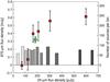 |
Fig. 9 Results from the stacking analysis in MS 1054-03, AC 114 and Abell 2744, as described in Sect. 5.2. Boxes: measured flux density in the maps when dividing the 24 μm positions into six equal parts, and stacking them. The stacked flux densities are measured by fitting a circular Gaussian to the maps, except in the lowest two 24 μm flux bins where no significant stacked signal was detected, and we instead measured the flux density in a circular aperture with the diameter of the beam FWHM. Circle: the stacked signal for all three clusters. Shaded bars: histograms indicating the distribution of 24 μm flux densities within each of the six flux bins. Each of the bins have two bars and the different shades of gray discriminate between them. In the highest flux bin the rightmost bar includes all the 24 μm sources with flux densities larger than 650 μJy. All flux values were corrected for gravitational magnification. |
So far, we have investigated the signal resulting by stacking LABOCA sub-map at each MIPS position within the fields. However, it is not plausible that all MIPS sources contribute equally to the stacked map. By choosing subsets of the total MIPS catalog with different 24 μm flux values, we examine a possible correlation between the flux density of the stacked signal and the 24 μm flux density. We perform this analysis in the fields of MS 1054-03, AC 114 and Abell 2744. There are 918 24 μm sources in the three fields. We divide the catalog into six sub-catalogs with equal number of sources (138), with median 24 μm flux densities of 72, 121, 164, 207, 303 and 599 μJy, and perform the stacking analysis for each of them. Both the 24 and 870 μm fluxes are demagnified. We find significant signals in the four highest 24 μm flux bins. The results are plotted in Fig. 9. At low 24 μm flux (S24 μm < 300 μJy) we find a linear relation between the 24 μm and the 870 μm flux. At higher flux densities a turnover occurs and the curve flattens out. The results are along the same lines as those of Greve et al. (2010) who find a flattening of the S24 μm–S870 μm relation at S24 μm ~ 350 μJy, in their stacking analysis.
Greve et al. (2010) argue that the linear relation at low MIPS fluxes is an indication that those sources are dominated by star formation, whereas the flattening of the curve at larger 24 μm fluxes is due to contamination by active galactic nuclei (AGN). The mid-IR flux is sensitive to warm dust, which is likely to be heated by an AGN. The 870 μm flux is more sensitive to colder dust, heated by starbursts. While the mid-IR flux increases the 870 μm flux stays constant, because it is not sensitive to the warm dust emission.
5.3. A MIPS source contributing to the stacked signal
It is beyond the scope of this paper to present a full multi-wavelength analysis and comparison between the MIPS and LABOCA maps. Here, we note one source which has a large magnification and is almost detected in the LABOCA map. Rigby et al. (2008) presented Spitzer/IRS spectroscopy of lensed galaxies, and discussed one source in the center of AC 114, gravitationally magnified by a factor of 9.7, and at a redshift of z = 1.47. At this position in our LABOCA map there is a positive signal with a significance of 3.4σ and flux density ~4 mJy.
Figure 10 shows a postage-stamp cutout of the region around the source. The LABOCA counterpart to the Spitzer source is just below our detection limit, and we would need more data to confirm it. If the 870 μm source is real, the high magnfication value would mean that its intrinsic flux density S870 μm < 0.5 mJy. We note that our lensing model for AC 114 gives a magnification value of μ = 6 for the Spitzer source position. Given that it lies very close to the brightest cluster galaxy in AC 114, the small discrepancy between the two magnification values are likely due to the lack of modeling of individual cluster member galaxies in this work.
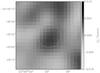 |
Fig. 10 Postage stamp cutout of the core in AC 114. The circle (with diameter of the angular resolution of the LABOCA map, FWHM = 27.5″) denotes the position of the Spitzer source at z = 1.47, as reported by Rigby et al. (2008). |
6. Contribution to the extragalactic background light
We have described and quantified the submm emission from two types of objects in the paper: the significantly detected sources in the maps, and those whose mean flux density is inferred from the stacking analysis. We now estimate the fraction of the Extragalactic Background Light (EBL) detected in the far-infrared by COBE (Puget et al. 1996; Fixsen et al. 1998; Dwek et al. 1998) that our survey has resolved. At 870 μm the surface brightness of the EBL is 44 ± 15 Jy deg-2 (Greve et al. 2010).
The total flux density of the detected submm sources that lie within the 10 arcmin central region is ~250 mJy. This corresponds to a surface brightness of 2.3 Jy deg-2, thus showing that the LABOCA observations have resolved ~5% of the EBL into significant > 3.5σ-sources. Another way to calculate the contribution to the EBL is to use the number counts, which have been corrected for completeness. Integrating the number counts yields a surface brightness of 5.7 Jy deg-2, corresponding to ~13% of the EBL.
Turning to the stacked signal, where we detected a mean observed flux density of 535 ± 37 μJy at 1278 positions in an area of ~500 arcmin2, the surface brightness is ~4.9 Jy deg-2 and the stacked submm signal thus corresponds to 11% of the EBL. Thus, in total our observations have uncovered the source of 24% of the EBL. Because gravitational lensing preserves surface brightness we can choose to perform this calculation using either the observed or intrinsic flux densities and areas.
Other authors find different EBL contributions. Knudsen et al. (2008) find that their observations resolve almost all of the extragalactic background light, since they discovered seven galaxies with sub-mJy intrinsic flux levels, and thus probe the number counts very deeply. Greve et al. (2010) find that the contribution for the stacked signal in the Extended Chandra Deep Field-South varies with redshift between 10% at z = 0.5 to 40% at z = 2.
7. Conclusions
We used the LABOCA receiver on APEX to carry out a submm survey of five clusters of galaxies. The clusters act as gravitational lenses and magnify background sources. The main results of the survey are summarized below.
-
1.
We discovered 37 submm sources, out of which 14 are newsubmm detections.
-
2.
We modeled the galaxy clusters as superpositions of spherical NFW halos and generated magnification maps for the five clusters.
-
3.
The magnification maps were used to correct for the gravitational lensing and to obtain the intrinsic flux densities of the detected sources.
-
4.
We constructed number counts taking into account both the gravitational lensing and the varying completeness level. The number counts are consistent with previous work within the uncertainties.
-
5.
We performed a stacking analysis in the LABOCA maps on positions of detected 24 μm sources in the fields. The stacking yields > 4.9σ detections in all fields with MIPS coverage, reaching noise levels below 100 μJy, more than an order of magnitude deeper than the individual maps.
-
6.
By dividing the 24 μm catalog in MS 1054-03, AC 114 and Abell 2744 into six equal halves, we find a linear relation between S24 μm and S870 μm at low 24 μm fluxes, followed by a flattening of the relation at S24 μm ~ 300 μJy. This behavior can be explained if the low MIPS fluxes trace star formation while the higher values are dominated by AGN heating.
-
7.
The observations reveal a total of ~24% of the infrared extragalactic background light, where ~13% comes from the significant submm sources and ~11% comes from the stacked signal.
We used Ned Wright’s cosmology calculator (Wright 2006) available at http://www.astro.ucla.edu/~wright/cosmocalc.html.
Clustering of faint submm sources has been observed in several studies (see e.g. Greve et al. 2004; Scott et al. 2006; Weiß et al. 2009), but at a resolution of 27.5″ the confusion noise contribution from clustering is much smaller than that from the “normal” Poisson distributed confusion noise (Negrello et al. 2004), and can therefore safely be neglected.
See the Fig. A1 in Johansson et al. (2010) for an illustration of these operations.
Acknowledgments
We would like to thank the APEX staff for excellent support during the observations. We also thank Rodrigo Parra for his help during observations of Abell 2744 in June 2008. We thank Martin Sommer for supplying us with his data on Abell 2163 and Eiichi Egami for letting us use his catalog of MIPS source in the Bullet Cluster field. We would like to thank Kirsten Knudsen for helpful discussions. We acknowledge support from the Swedish research council (Vetenskapsrådet). We thank the referee for very useful comments.
This work is based in part on observations made with the Spitzer Space Telescope, which is operated by the Jet Propulsion Laboratory, California Institute of Technology under a contract with NASA. This research has made use of the NASA/IPAC Extragalactic Database (NED) which is operated by the Jet Propulsion Laboratory, California Institute of Technology, under contract with the National Aeronautics and Space Administration. This research has also made use of NASA’s Astrophysics Data System Bibliographic Services.
References
- Austermann, J. E., Dunlop, J. S., Perera, T. A., et al. 2010, MNRAS, 401, 160 [NASA ADS] [CrossRef] [Google Scholar]
- Barger, A. J., Cowie, L. L., & Sanders, D. B. 1999, ApJ, 518, L5 [NASA ADS] [CrossRef] [Google Scholar]
- Beelen, A., Omont, A., Bavouzet, N., et al. 2008, A&A, 485, 645 [NASA ADS] [CrossRef] [EDP Sciences] [Google Scholar]
- Bertoldi, F., Carilli, C., Aravena, M., et al. 2007, ApJS, 172, 132 [NASA ADS] [CrossRef] [Google Scholar]
- Blain, A. W., Smail, I., Ivison, R. J., Kneib, J.-P., & Frayer, D. T. 2002, Phys. Rep., 369, 111 [NASA ADS] [CrossRef] [Google Scholar]
- Borys, C., Chapman, S., Halpern, M., & Scott, D. 2003, MNRAS, 344, 385 [NASA ADS] [CrossRef] [Google Scholar]
- Boschin, W., Girardi, M., Spolaor, M., & Barrena, R. 2006, A&A, 449, 461 [NASA ADS] [CrossRef] [EDP Sciences] [Google Scholar]
- Bryan, G. L., & Norman, M. L. 1998, ApJ, 495, 80 [NASA ADS] [CrossRef] [Google Scholar]
- Bullock, J. S., Kolatt, T. S., Sigad, Y., et al. 2001, MNRAS, 321, 559 [Google Scholar]
- Campusano, L. E., Pelló, R., Kneib, J., et al. 2001, A&A, 378, 394 [NASA ADS] [CrossRef] [EDP Sciences] [Google Scholar]
- Chapman, S. C., Scott, D., Borys, C., & Fahlman, G. G. 2002a, MNRAS, 330, 92 [NASA ADS] [CrossRef] [Google Scholar]
- Chapman, S. C., Smail, I., Ivison, R. J., & Blain, A. W. 2002b, MNRAS, 335, L17 [NASA ADS] [CrossRef] [Google Scholar]
- Chapman, S. C., Blain, A. W., Smail, I., & Ivison, R. J. 2005, ApJ, 622, 772 [NASA ADS] [CrossRef] [Google Scholar]
- Clowe, D., Luppino, G. A., Kaiser, N., & Gioia, I. M. 2000, ApJ, 539, 540 [NASA ADS] [CrossRef] [Google Scholar]
- Clowe, D., Gonzalez, A., & Markevitch, M. 2004, ApJ, 604, 596 [NASA ADS] [CrossRef] [Google Scholar]
- Condon, J. J. 1974, ApJ, 188, 279 [NASA ADS] [CrossRef] [Google Scholar]
- Coppin, K., Halpern, M., Scott, D., Borys, C., & Chapman, S. 2005, MNRAS, 357, 1022 [NASA ADS] [CrossRef] [Google Scholar]
- Coppin, K., Chapin, E. L., Mortier, A. M. J., et al. 2006, MNRAS, 372, 1621 [NASA ADS] [CrossRef] [Google Scholar]
- Danielson, A. L. R., Swinbank, A. M., Smail, I., et al. 2010, MNRAS, 1565 [Google Scholar]
- De Breuck, C., Neri, R., Morganti, R., et al. 2003, A&A, 401, 911 [NASA ADS] [CrossRef] [EDP Sciences] [Google Scholar]
- Dole, H., Lagache, G., Puget, J., et al. 2006, A&A, 451, 417 [NASA ADS] [CrossRef] [EDP Sciences] [MathSciNet] [Google Scholar]
- Dunne, L., Ivison, R. J., Maddox, S., et al. 2009, MNRAS, 394, 3 [NASA ADS] [CrossRef] [Google Scholar]
- Dwek, E., Arendt, R. G., Hauser, M. G., et al. 1998, ApJ, 508, 106 [NASA ADS] [CrossRef] [Google Scholar]
- Egami, E., Rex, M., Rawle, T. D., et al. 2010, A&A, 518, L12 [CrossRef] [EDP Sciences] [Google Scholar]
- Ettori, S., Gastaldello, F., Leccardi, A., et al. 2010, A&A, 524, A68 [NASA ADS] [CrossRef] [EDP Sciences] [Google Scholar]
- Fahlman, G., Kaiser, N., Squires, G., & Woods, D. 1994, ApJ, 437, 56 [NASA ADS] [CrossRef] [Google Scholar]
- Fixsen, D. J., Dwek, E., Mather, J. C., Bennett, C. L., & Shafer, R. A. 1998, ApJ, 508, 123 [NASA ADS] [CrossRef] [Google Scholar]
- Gehrels, N. 1986, ApJ, 303, 336 [NASA ADS] [CrossRef] [Google Scholar]
- Gonzalez, A. H., Clowe, D., Bradač, M., et al. 2009, ApJ, 691, 525 [NASA ADS] [CrossRef] [Google Scholar]
- Gonzalez, A. H., Papovich, C., Bradač, M., & Jones, C. 2010, ApJ, 720, 245 [NASA ADS] [CrossRef] [Google Scholar]
- Greve, T. R., Ivison, R. J., Bertoldi, F., et al. 2004, MNRAS, 354, 779 [NASA ADS] [CrossRef] [Google Scholar]
- Greve, T. R., Weiß, A., Walter, F., et al. 2010, ApJ, 719, 483 [NASA ADS] [CrossRef] [Google Scholar]
- Güsten, R., Nyman, L. Å., Schilke, P., et al. 2006, A&A, 454, L13 [NASA ADS] [CrossRef] [EDP Sciences] [Google Scholar]
- Hoekstra, H., Franx, M., & Kuijken, K. 2000, ApJ, 532, 88 [NASA ADS] [CrossRef] [Google Scholar]
- Hogg, D. W. 2001, AJ, 121, 1207 [NASA ADS] [CrossRef] [Google Scholar]
- Hogg, D. W., & Turner, E. L. 1998, PASP, 110, 727 [NASA ADS] [CrossRef] [Google Scholar]
- Ikarashi, S., Kohno, K., Aguirre, J. E., et al. 2010, [arXiv:1009.1455] [Google Scholar]
- Johansson, D., Horellou, C., Sommer, M. W., et al. 2010, A&A, 514, A77 [NASA ADS] [CrossRef] [EDP Sciences] [Google Scholar]
- Knudsen, K. K., van der Werf, P., Franx, M., et al. 2005, ApJ, 632, L9 [NASA ADS] [CrossRef] [Google Scholar]
- Knudsen, K. K., Barnard, V. E., van der Werf, P. P., et al. 2006, MNRAS, 368, 487 [NASA ADS] [CrossRef] [Google Scholar]
- Knudsen, K. K., van der Werf, P. P., & Kneib, J.-P. 2008, MNRAS, 384, 1611 [NASA ADS] [CrossRef] [Google Scholar]
- Kovács, A. 2008, in Presented at the Society of Photo-Optical Instrumentation Engineers (SPIE) Conf., 7020 [Google Scholar]
- Maurogordato, S., Cappi, A., Ferrari, C., et al. 2008, A&A, 481, 593 [NASA ADS] [CrossRef] [EDP Sciences] [Google Scholar]
- Natarajan, P., Kneib, J., Smail, I., & Ellis, R. S. 1998, ApJ, 499, 600 [NASA ADS] [CrossRef] [Google Scholar]
- Navarro, J. F., Frenk, C. S., & White, S. D. M. 1997, ApJ, 490, 493 [NASA ADS] [CrossRef] [Google Scholar]
- Negrello, M., Magliocchetti, M., Moscardini, L., et al. 2004, MNRAS, 352, 493 [NASA ADS] [CrossRef] [Google Scholar]
- Negrello, M., Hopwood, R., De Zotti, G., et al. 2010, Science, 330, 800 [NASA ADS] [CrossRef] [Google Scholar]
- Nord, M., Basu, K., Pacaud, F., et al. 2009, A&A, 506, 623 [NASA ADS] [CrossRef] [EDP Sciences] [Google Scholar]
- Omont, A., Cox, P., Bertoldi, F., et al. 2001, A&A, 374, 371 [NASA ADS] [CrossRef] [EDP Sciences] [Google Scholar]
- Patanchon, G., Ade, P. A. R., Bock, J. J., et al. 2009, ApJ, 707, 1750 [NASA ADS] [CrossRef] [EDP Sciences] [Google Scholar]
- Pérez-González, P. G., Egami, E., Rex, M., et al. 2010, A&A, 518, L15 [NASA ADS] [CrossRef] [EDP Sciences] [Google Scholar]
- Puget, J.-L., Abergel, A., Bernard, J.-P., et al. 1996, A&A, 308, L5 [NASA ADS] [Google Scholar]
- Radovich, M., Puddu, E., Romano, A., Grado, A., & Getman, F. 2008, A&A, 487, 55 [NASA ADS] [CrossRef] [EDP Sciences] [Google Scholar]
- Rex, M., Ade, P. A. R., Aretxaga, I., et al. 2009, ApJ, 703, 348 [NASA ADS] [CrossRef] [Google Scholar]
- Rex, M., Rawle, T. D., Egami, E., et al. 2010, A&A, 518, L13 [NASA ADS] [CrossRef] [EDP Sciences] [Google Scholar]
- Rieke, G. H., Young, E. T., Engelbracht, C. W., et al. 2004, ApJS, 154, 25 [NASA ADS] [CrossRef] [Google Scholar]
- Rigby, J. R., Marcillac, D., Egami, E., et al. 2008, ApJ, 675, 262 [NASA ADS] [CrossRef] [Google Scholar]
- Schechter, P. 1976, ApJ, 203, 297 [Google Scholar]
- Scott, K. S., Austermann, J. E., Perera, T. A., et al. 2008, MNRAS, 385, 2225 [NASA ADS] [CrossRef] [Google Scholar]
- Scott, K. S., Yun, M. S., Wilson, G. W., et al. 2010, MNRAS, 405, 2260 [NASA ADS] [Google Scholar]
- Scott, S. E., Dunlop, J. S., & Serjeant, S. 2006, MNRAS, 370, 1057 [NASA ADS] [CrossRef] [Google Scholar]
- Scoville, N., Aussel, H., Brusa, M., et al. 2007, ApJS, 172, 1 [NASA ADS] [CrossRef] [Google Scholar]
- Siringo, G., Kreysa, E., Kovács, A., et al. 2009, A&A, 497, 945 [NASA ADS] [CrossRef] [EDP Sciences] [Google Scholar]
- Smail, I., Ivison, R. J., & Blain, A. W. 1997, ApJ, 490, L5 [NASA ADS] [CrossRef] [Google Scholar]
- Smail, I., Ivison, R. J., Blain, A. W., & Kneib, J.-P. 2002, MNRAS, 331, 495 [NASA ADS] [CrossRef] [Google Scholar]
- Swinbank, A. M., Smail, I., Longmore, S., et al. 2010, Nature, 464, 733 [Google Scholar]
- Tacconi, L. J., Neri, R., Chapman, S. C., et al. 2006, ApJ, 640, 228 [NASA ADS] [CrossRef] [Google Scholar]
- Takada, M., & Jain, B. 2003, MNRAS, 344, 857 [NASA ADS] [CrossRef] [Google Scholar]
- Vieira, J. D., Crawford, T. M., Switzer, E. R., et al. 2010, ApJ, 719, 763 [NASA ADS] [CrossRef] [Google Scholar]
- Wardlow, J. L., Smail, I., Wilson, G. W., et al. 2010, MNRAS, 401, 2299 [NASA ADS] [CrossRef] [Google Scholar]
- Weiß, A., Kovács, A., Coppin, K., et al. 2009, ApJ, 707, 1201 [NASA ADS] [CrossRef] [Google Scholar]
- Wilson, G. W., Austermann, J. E., Perera, T. A., et al. 2008a, MNRAS, 386, 807 [Google Scholar]
- Wilson, G. W., Hughes, D. H., Aretxaga, I., et al. 2008b, MNRAS, 390, 1061 [NASA ADS] [CrossRef] [Google Scholar]
- Wright, E. L. 2006, PASP, 118, 1711 [NASA ADS] [CrossRef] [Google Scholar]
- Zemcov, M., Borys, C., Halpern, M., Mauskopf, P., & Scott, D. 2007, MNRAS, 376, 1073 [NASA ADS] [CrossRef] [Google Scholar]
Appendix A: Comparison with other submm observations
MS 1054-03
Even though the galaxy clusters in our sample have been well studied across the electromagnetic spectrum, submm maps have been published for only one system, MS 1054-03 (Knudsen et al. 2008, hereafter K08) using SCUBA. Subsets of those SCUBA data were previously analyzed by Chapman et al. 2002a; Zemcov et al. 2007; Knudsen et al. 2005, with mostly similar source catalogs. Differences in the SCUBA source catalogs are discussed by K08. We will now compare our catalog for MS 1054-03 with theirs.
K08 reach a noise level of 0.86 mJy beam-1 in the deepest part of the map, while their area-weighted noise level is 1.49 mJy beam-1. They detect nine significant sources in their map. The noise level in the LABOCA map in the central part of the map is 1.3 mJy beam-1 (see Fig. 2), while the average noise level within the central 10′ is 1.6 mJy beam-1. The SCUBA map covers the cluster region (14.4 arcmin2) while the usable map area in the LABOCA map is ~150 arcmin2.
Only one of our detected sources lies in the area covered by K08. It is extended with respect to the LABOCA beam, and has an angular size of 30″ × 35″. Its flux density is 9.8 ± 1.8 mJy. In the same area, K08 report three sources, separated by of 25.3″, 25.8″ and 18.0″. LABOCA, with a coarser resolution than SCUBA, causes the three sources to blend together. We compared the measured LABOCA source size with a simple model of the three K08-sources, constructed as a sum of three LABOCA beam shaped Gaussians (angular FWHM 19.5″). We then smoothed this model image with a Gaussian of angular maps. The fitted source has an angular size of 33″ × 40″. The slightly larger angular size of the model compared to the observed LABOCA source can be explained with uncertainties in the fitted FWHMs and in the SCUBA and LABOCA positions. The sum of the flux density of the three SCUBA sources, scaled from 850 μm to 870 μm with a submm spectral index of 2.7, is 11.9 ± 1.5 mJy. This is within the 1σ uncertainty interval of the LABOCA flux measurement.
The other six sources detected by K08 have 850 μm flux densities that, when extrapolated to 870 μm, are too faint to be detected in the LABOCA map.
Abell 2163
Nord et al. (2009) presented the first LABOCA map of a galaxy cluster detected in the Sunyaev–Zeldovich increment, Abell 2163. A bright point source close to the cluster center, with a flux density of 11.9 ± 1.9 mJy, was noted, but not discussed. Using the same data set as in Nord et al., but filtering out most of the extended SZ-signal, we detect the same point source in our map, with a flux density of 8.9 ± 2 mJy.
1E 0657-56
The brightest submm source in the Bullet Cluster has been thoroughly discussed (see Johansson et al. 2010 and references therein). Submm and FIR observations by the SPIRE and PACS instruments on the Herschel satellite show counterparts of LABOCA sources (Rex et al. 2010; Pérez-González et al. 2010) as part of the Herschel Lensing Survey (Egami et al. 2010).
All Tables
Flux densities and magnification factors for submm sources detected in the survey.
All Figures
|
Fig. 1 Signal-to-noise maps of the five cluster fields. White circles represent the significant sources in the map and black contours show the noise maps of each cluster map at levels of 2, 4 and 8 mJy beam-1. The signal-to-noise representation causes the appearance of the increasing noise towards the edge of each map to be suppressed. |
| In the text | |
|
Fig. 2 Pixel-to-pixel root-mean-square (rms) as a function of radial distance from the map center for the five cluster fields, described in Sect. 3.2. |
| In the text | |
|
Fig. 3 Completeness of the five cluster fields as a function of flux density, as described in Sect. 3.2. |
| In the text | |
|
Fig. 4 Magnification maps for the five clusters. The positions of the detected submm sources are marked on the maps with circles. |
| In the text | |
|
Fig. 5 Square-root of the area with magnification > μ as function of magnification (μ) for the five cluster models in the sample. |
| In the text | |
|
Fig. 6 Derived number counts for the survey (filled boxes) compared with results from previous observations. |
| In the text | |
|
Fig. 7 Stacked 870 μm maps (in units of mJy beam-1) on the 24 μm positions for the cluster fields with MIPS observations, overlaid with signal-to-noise contours. The white contours range between 3σ and 13σ with an increment of 2σ, while the black countours show the − 3σ level. The maps have not been corrected for gravitational magnification. The fifth map is the coadded signal of the four individual stacked maps, which yields a 14.5σ-detection. In Table 6 we present fits to the stacked maps. |
| In the text | |
|
Fig. 8 Top panel: normalized histogram of the signal-to-noise values in the LABOCA maps at the 24 μm positions (dash-dotted line), compared with the mean histogram from 20 sets of random positions (solid line). Lower panel: difference signal between the signal-to-noise histogram above, showing that the main part of the stacked signal is due to sources with signal-to-noise ratios between 0.5 and 2. This histogram clearly shows a deficit of points at negative signal-to-noise units and an excess at positive signal-to-noise units. |
| In the text | |
|
Fig. 9 Results from the stacking analysis in MS 1054-03, AC 114 and Abell 2744, as described in Sect. 5.2. Boxes: measured flux density in the maps when dividing the 24 μm positions into six equal parts, and stacking them. The stacked flux densities are measured by fitting a circular Gaussian to the maps, except in the lowest two 24 μm flux bins where no significant stacked signal was detected, and we instead measured the flux density in a circular aperture with the diameter of the beam FWHM. Circle: the stacked signal for all three clusters. Shaded bars: histograms indicating the distribution of 24 μm flux densities within each of the six flux bins. Each of the bins have two bars and the different shades of gray discriminate between them. In the highest flux bin the rightmost bar includes all the 24 μm sources with flux densities larger than 650 μJy. All flux values were corrected for gravitational magnification. |
| In the text | |
|
Fig. 10 Postage stamp cutout of the core in AC 114. The circle (with diameter of the angular resolution of the LABOCA map, FWHM = 27.5″) denotes the position of the Spitzer source at z = 1.47, as reported by Rigby et al. (2008). |
| In the text | |
Current usage metrics show cumulative count of Article Views (full-text article views including HTML views, PDF and ePub downloads, according to the available data) and Abstracts Views on Vision4Press platform.
Data correspond to usage on the plateform after 2015. The current usage metrics is available 48-96 hours after online publication and is updated daily on week days.
Initial download of the metrics may take a while.