| Issue |
A&A
Volume 527, March 2011
|
|
|---|---|---|
| Article Number | A106 | |
| Number of page(s) | 11 | |
| Section | Astronomical instrumentation | |
| DOI | https://doi.org/10.1051/0004-6361/201016082 | |
| Published online | 04 February 2011 | |
Revisiting the radio interferometer measurement equation
I. A full-sky Jones formalism
Netherlands Institute for Radio Astronomy (ASTRON) PO Box 2,
7990AA
Dwingeloo,
The Netherlands
e-mail: This email address is being protected from spambots. You need JavaScript enabled to view it.
Received:
5
November
2010
Accepted:
5
January
2011
Abstract
Context. Since its formulation by Hamaker et al., the radio interferometer measurement equation (RIME) has provided a rigorous mathematical basis for the development of novel calibration methods and techniques, including various approaches to the problem of direction-dependent effects (DDEs). However, acceptance of the RIME in the radio astronomical community at large has been slow, which is partially due to the limited availability of software to exploit its power, and the sparsity of practical results. This needs to change urgently.
Aims. This series of papers aims to place recent developments in the treatment of DDEs into one RIME-based mathematical framework, and to demonstrate the ease with which the various effects can be described and understood. It also aims to show the benefits of a RIME-based approach to calibration.
Methods. Paper I re-derives the RIME from first principles, extends the formalism to the full-sky case, and incorporates DDEs. Paper II then uses the formalism to describe self-calibration, both with a full RIME, and with the approximate equations of older software packages, and shows how this is affected by DDEs. It also gives an overview of real-life DDEs and proposed methods of dealing with them. Finally, in Paper III some of these methods are exercised to achieve an extremely high-dynamic range calibration of WSRT observations of 3C 147 at 21 cm, with full treatment of DDEs.
Results. The RIME formalism is extended to the full-sky case (Paper I), and is shown to be an elegant way of describing calibration and DDEs (Paper II). Applying this to WSRT data (Paper III) results in a noise-limited image of the field around 3C 147 with a very high dynamic range (1.6 million), and none of the off-axis artifacts that plague regular selfcal. The resulting differential gain solutions contain significant information on DDEs and errors in the sky model.
Conclusions. The RIME is a powerful formalism for describing radio interferometry, and underpins the development of novel calibration methods, in particular those dealing with DDEs. One of these is the differential gains approach used for the 3C 147 reduction. Differential gains can eliminate DDE-related artifacts, and provide information for iterative improvements of sky models. Perhaps most importantly, sources as faint as 2 mJy have been shown to yield meaningful differential gain solutions, and thus can be used as potential calibration beacons in other DDE-related schemes.
Key words: methods: numerical / methods: analytical / methods: data analysis / techniques: interferometric / techniques: polarimetric
© ESO, 2011
Introduction to the series
The measurement equation of a generic radio interferometer (henceforth referred to as the RIME) was formulated by Hamaker et al. (1996) after almost 50 years of radio astronomy. Prior to the RIME, mathematical models of radio interferometers (as implemented by a number of software packages such as AIPS, Miriad, NEWSTAR, DIFMAP) were somewhat ad hoc and approximate. Despite this (and in part thanks to the careful design of existing instruments), the technique of self-calibration (Cornwell & Wilkinson 1981) has allowed radio astronomers to achieve spectacular results. However, by the time the RIME was formulated, even older and well-understood instruments such as the Westerbork Synthesis Radio Telescope (WSRT) and the Very Large Array (VLA) were beginning to expose the limitations of these approximate models. New instruments (and upgrades of older observatories), such as the current crop of Square Kilometer Array (Schilizzi 2004) “pathfinders”, and indeed the SKA itself, were already beginning to loom on the horizon. These new instruments exhibit far more subtle and elaborate observational effects, due not only to their greatly increased sensitivity, but also to new features of their design. In particular, while traditional selfcal only deals with direction-independent effects (DIEs), calibration of these new instruments requires us to deal with direction-dependent effects (DDEs), or effects that vary across the field of view (FoV) of the instrument. Following Noordam & Smirnov (2010), I shall refer to generations of calibration methods, with first-generation calibration (1GC) predating selfcal, 2GC being traditional selfcal as implemented by the aforementioned packages, and 3GC corresponding to the burgeoning field of DDE-related methods and algorithms.
It is indeed quite fortunate that the emergence of the RIME formalism has provided us with a complete and elegant mathematical framework for dealing with observational effects, and ultimately DDEs. Oddly enough, outside of a small community of algorithm developers that have enthusiastically accepted the formalism and put it to good use, uptake of RIME by radio astronomers at large has been slow. Even more worryingly, almost 15 years after the first publication, the formalism is hardly ever taught to the new generation of students. This is worrying, because in my estimation, the RIME should be the cornerstone of every entry-level interferometry course! In part, this slow acceptance has been shaped by the availability of software. Today’s radio astronomers rely almost exclusively on the 2GC software packages mentioned above, whose internal paradigms are rooted in the selfcal developments of the 1980s and lack an explicit RIME1. On the other hand, relatively few observations were really sensitive enough to push the limits of (or have their science goals compromised by) 2GC. The continued success of legacy packages has meant that the thinking about interferometry and calibration has still been largely shaped by pre-RIME paradigms. What has not helped this situation is that new software exploiting the power of the RIME has been slow to emerge, and practical results even more so – but see Paper III (Smirnov 2011b) of this series.
On the other hand, from my personal experience of teaching the RIME at several workshops, once the penny drops, people tend to describe it in terms such as “obvious”, “simple”, “intuitive”, “elegant” and “powerful”. This points at an explanatory gap in the literature. Paper I of this series therefore tries to address this gap, recasting existing ideas into one consistent mathematical framework, and showing where other approaches to the RIME fit in. It first revisits the ideas of the original RIME papers (Hamaker et al. 1996; Hamaker 2000), deriving the RIME from first principles. It then demonstrates how the fundamentals of interferometry itself (and the van Cittert-Zernike theorem in particular) follow from the RIME (rather than the other way around!), in the process showing how the formalism can incorporate DDEs. This section also looks at alternative formulations of the RIME and their practical implications, and shows where they fit into the formalism. It also tries to clear up some controversies and misunderstandings that have accumulated over the years. Paper II (Smirnov 2011a) then discusses calibration in RIME terms, and explicates the links between the RIME and 2GC implementations of selfcal.
Paper II also discusses the subject of DDEs, and places existing approaches into the mathematical framework developed in the preceding sections. DDEs were outside the scope of the original RIME publications, but various authors have been incorporating them into the RIME since. Rau et al. (2009) and Bhatnagar (2009) provide an in-depth review of these developments, especially as pertaining to imaging and deconvolution. The above authors have developed a description of DDEs using the 4 × 4 Mueller matrix and coherency vector formalism of the first RIME paper by Hamaker et al. (1996). The 4 × 4 formalism has also been included in the 2nd edition of Thompson et al. (2001, Sect. 4.8). In the meantime, Hamaker (2000) has recast the RIME using only 2 × 2 matrices. The 2 × 2 form of the RIME has far more intuitive appeal2, and is far better suited for describing calibration problems, yet has been somewhat unjustly ignored in the literature. Addressing this perceived injustice is yet another aim of these papers. (Section 6 describes the 4 × 4 vs. 2 × 2 formalisms in more detail.)
Last but certainly not least, Paper III (Smirnov 2011b) shows an application of these concepts to real data. It presents a record dynamic range (over 1.6 million) calibration of a WSRT observation, including calibration of DDEs. It then analyzes the results of this calibration, shows how the calibration solutions can be used to improve sky models, and demonstrates a rather important implication for the calibratability of future telescopes.
1. The RIME of a single source
Like many crucial insights, the RIME seems perfectly obvious and simple in hindsight. In fact, it can be almost trivially derived from basic considerations of signal propagation, as shown by Hamaker et al. (1996). In this paper, I will essentially repeat and elaborate on this derivation. This is not original work, but there are several good reasons for reiterating the full argument, as opposed to simply referring back to the original RIME papers. Firstly, some aspects of the basic RIME noted here are not covered by the original papers at all. These are the commutation considerations of Sect. 1.6, the fact that Jones matrices and coherency matrices behave differently under coordinate transforms (for which reason I even propose a different typographical convention for them), as discussed in Sect. 6.3, and the 1/2-vs.-1 controversy of Sect. 7.2. Then there’s the fact that the 2 × 2 version of the formalism proposed by Hamaker (2000) and and employed here provides for a much clearer and more intuitive picture that the original 4 × 4 derivation (see Sect. 6.1 for a discussion), and so deserves far more exposure in the literature than the sole Hamaker paper to date. Finally, I want to establish some typographical conventions and mathematical nomenclature, and lay the groundwork for my own extensions of the formalism, which start at Sect. 3. This seemed sufficient reason to give a complete derivation of the RIME from scratch.
In Sects. 2 and 3, I extend the 2 × 2 formalism into the image-plane domain, show how the van Cittert-Zernike (VCZ) theorem naturally follows from the RIME, and sketch the problem of DDEs. Section 4 elaborates some RIME-based closure relationships, Sect. 5 then examines some important limitations and boundaries of the RIME formalism, and Sect. 6 looks at alternative formulations of the RIME. Finally, Sect. 7 attempts to clear up some errors and controversies surrounding the formalism.
1.1. Signal propagation
Consider a single source of quasi-monochromatic signal (i.e. a sky consisting of a single point source). The signal at a fixed point in space and time can be then be described by the complex vector e. Let us pick an orthonormal xyz coordinate system, with z along the direction of propagation (i.e. from antenna to source). In such a system, e can be represented by a column vector of 2 complex numbers:
 Our fundamental
assumption is linearity: all transformations along the signal path are
linear w.r.t. e. Basic linear algebra tells us that all
linear transformations of a 2-vector can be represented (in any given coordinate system)
by a matrix multiplication:
Our fundamental
assumption is linearity: all transformations along the signal path are
linear w.r.t. e. Basic linear algebra tells us that all
linear transformations of a 2-vector can be represented (in any given coordinate system)
by a matrix multiplication:
 where
J is a 2 × 2 complex matrix known as the Jones
matrix (Jones 1941). Obviously, multiple
effects along the signal propagation path correspond to repeated matrix multiplications,
forming what I call a Jones chain. We can regard multiple effects
separately and write out Jones chains, or we can collapse them all into a single
cumulative Jones matrix as convenient:
where
J is a 2 × 2 complex matrix known as the Jones
matrix (Jones 1941). Obviously, multiple
effects along the signal propagation path correspond to repeated matrix multiplications,
forming what I call a Jones chain. We can regard multiple effects
separately and write out Jones chains, or we can collapse them all into a single
cumulative Jones matrix as convenient: 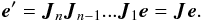 (1)The order of terms in
a Jones chain corresponds to the physical order in which the effects occur along the
signal path. Since matrix multiplication does not (in general) commute, we must be careful
to preserve this order in our equations.
(1)The order of terms in
a Jones chain corresponds to the physical order in which the effects occur along the
signal path. Since matrix multiplication does not (in general) commute, we must be careful
to preserve this order in our equations.
Now, the signal hits our antenna and is ultimately converted into complex voltages by the
antenna feeds. Let us further assume that we have two feeds a and
b (for example, two linear dipoles, or left/right circular feeds), and
that the voltages va and
vb are linear w.r.t.
e. We can formally treat the two voltages as a voltage
vector v, analogous to e.
Their linear relationship is yet another matrix multiplication:  (2)Equation (2) can be thought of as representing the
fundamental linear relationship between the voltage vector v
as measured by the antenna feeds, and the “original” signal vector
e at some arbitrarily distant point, with
J being the cumulative product of all propagation
effects along the signal path (including electronic effects in the antenna/feed itself). I
shall call refer to this J as the total Jones
matrix, as distinct from the individual Jones terms in a Jones chain.
(2)Equation (2) can be thought of as representing the
fundamental linear relationship between the voltage vector v
as measured by the antenna feeds, and the “original” signal vector
e at some arbitrarily distant point, with
J being the cumulative product of all propagation
effects along the signal path (including electronic effects in the antenna/feed itself). I
shall call refer to this J as the total Jones
matrix, as distinct from the individual Jones terms in a Jones chain.
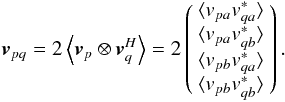
1.2. The visibility matrix
Two spatially separated antennas p and q measure two
independent voltage vectors
vp,vq.
In an interferometer, these are fed into a correlator, which produces 4
pairwise correlations between the components of
vp and
vq:  (3)Here, angle brackets
denote averaging over some (small) time and frequency bin, and
x∗ is the complex conjugate of x. It is
convenient for our purposes to arrange these four correlations into the visibility
matrix3 Vpq:
(3)Here, angle brackets
denote averaging over some (small) time and frequency bin, and
x∗ is the complex conjugate of x. It is
convenient for our purposes to arrange these four correlations into the visibility
matrix3 Vpq:
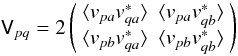 I
introduce a factor of 2 here, for reasons explained in Sect. 7.2. It is easily seen that Vpq can be
written as a matrix product of
vp (as a column vector), and
the conjugate of vq (as a row
vector):
I
introduce a factor of 2 here, for reasons explained in Sect. 7.2. It is easily seen that Vpq can be
written as a matrix product of
vp (as a column vector), and
the conjugate of vq (as a row
vector): 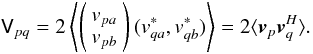 (4)Here,
H represents the conjugate transpose operation (also called a Hermitian
transpose).
(4)Here,
H represents the conjugate transpose operation (also called a Hermitian
transpose).
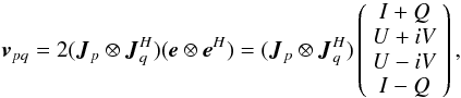
1.3. The RIME emerges
Starting with some arbitrarily distant vector e, our signal
travels along two different paths to antennas p and q.
Following Eq. (2), each propagation path
has its own total Jones matrix,
Jp and
Jq. Combining Eqs. (2) and (4), we get:  (5)Assuming that
Jp and
Jq are constant over the
averaging interval4, we can move them outside the
averaging operator:
(5)Assuming that
Jp and
Jq are constant over the
averaging interval4, we can move them outside the
averaging operator: 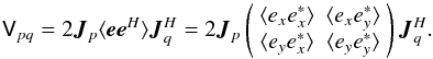 (6)The bracketed quantities
here are intimately related to the definition of the Stokes parameters (Born & Wolf 1964; Thompson et al. 2001). Hamaker
& Bregman (1996) explicitly show that
(6)The bracketed quantities
here are intimately related to the definition of the Stokes parameters (Born & Wolf 1964; Thompson et al. 2001). Hamaker
& Bregman (1996) explicitly show that 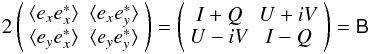 (7)I now
define the brightness matrix
(7)I now
define the brightness matrix  as the right-hand
side5 of Eq. (7). This gives us the first form of the RIME, that of a single point
source:
as the right-hand
side5 of Eq. (7). This gives us the first form of the RIME, that of a single point
source: 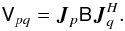 (8)Or in expanded form:
 which quite
elegantly ties together the observed visibilities Vpq with the
intrinsic source brightness , and the
per-antenna terms Jp and
Jq.
which quite
elegantly ties together the observed visibilities Vpq with the
intrinsic source brightness , and the
per-antenna terms Jp and
Jq.
Note that Eq. (8) holds in any coordinate
system. The vector e, the brightness matrix
that is derived
from it, and the linear transformations
Jp and
Jq are distinct mathematical
entities that are independent of coordinate systems; choosing a coordinate basis
associates a specific representation with
e, and
J, manifesting itself in a 2-vector or a 2 × 2 matrix
populated with specific complex numbers. For example, it is quite possible (and sometimes
desirable) to rewrite the RIME in a circular polarization basis. This is discussed further
in Sect. 6.3. In this paper, I shall use an
orthonormal xyz basis unless otherwise stated.
1.4. Some typographical conventions
Throughout this series of papers, I shall adopt the following typographical conventions for formulas:
-
Scalar quantities will be indicated by lower- and uppercaseitalics: ex,I,Kp.
-
Vectors will be indicated by lowercase bold italics: e.
-
Jones matrices will be indicated by uppercase bold italics: J. As a special case, scalar matrices (Sect. 1.6) will be indicated by normal-weight italics: Kp.
-
Visibility, coherency and brightness matrices will be indicated by sans-serif font:
 . This
emphasizes their different mathematical nature (and in particular, that they
transform differently under change of coordinate frame, Sect. 6.3).
. This
emphasizes their different mathematical nature (and in particular, that they
transform differently under change of coordinate frame, Sect. 6.3).
1.5. The “onion” form
We can also choose to expand Jp
and Jq into their associated
Jones chains, as per Eq. (1). This results
in the rather pleasing “onion” form of the RIME:  (9)Intuitively,
this corresponds to various effects in the signal path applying sequential layers of
“corruptions” to the original source brightness . Note that the two
signal paths can in principle be entirely dissimilar, making the “onion” asymmetric (hence
the use of n ≠ m for the outer indices). An example of
this is VLBI with ad hoc arrays composed of different types of telescopes. One of the
strengths of the RIME is its ability to describe heterogeneous interferometer arrays with
dissimilar signal propagation paths.
(9)Intuitively,
this corresponds to various effects in the signal path applying sequential layers of
“corruptions” to the original source brightness . Note that the two
signal paths can in principle be entirely dissimilar, making the “onion” asymmetric (hence
the use of n ≠ m for the outer indices). An example of
this is VLBI with ad hoc arrays composed of different types of telescopes. One of the
strengths of the RIME is its ability to describe heterogeneous interferometer arrays with
dissimilar signal propagation paths.
1.6. An elementary Jones taxonomy
Different propagation effects are described by different kinds of Jones matrices. The simplest kind of matrix is a scalar matrix, corresponding to a transformation that affects both components of the e vector equally. I shall use normal-weight italics (K) to emphasize scalar matrices. An example is the phase delay matrix below:
 An important property of
scalar matrices is that they have the same representation in all coordinate systems, so
scalarity is defined independently of coordinate frame.
An important property of
scalar matrices is that they have the same representation in all coordinate systems, so
scalarity is defined independently of coordinate frame.
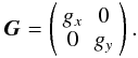
Diagonal matrices correspond to effects that affect the two e components independently, without intermixing. Note that unlike scalarness, diagonality does depend on choice of coordinate systems. For example, if we consider linear dipoles, their electronic gains are (nominally) independent, and the corresponding Jones matrix is diagonal in an xy coordinate basis:
 The gains of a pair of
circular receptors, on the other hand, are not diagonal in an xy frame
(but are diagonal in a circular polarization frame – see Sect. 6.3).
The gains of a pair of
circular receptors, on the other hand, are not diagonal in an xy frame
(but are diagonal in a circular polarization frame – see Sect. 6.3).
Matrices with non-zero off-diagonal terms intermix the two components of e. A special case of this is the rotation matrix:
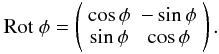 Like diagonality, the
property of being a rotation matrix also depends on choice of coordinate frame. Examples
of rotation matrices (in an xy frame) are rotation through parallactic
angle P, and Faraday rotation in the ionosphere
F. Note also that rotation in an xy
frame becomes a special kind of diagonal matrix in the circular frame (see Sect. 6.3).
Like diagonality, the
property of being a rotation matrix also depends on choice of coordinate frame. Examples
of rotation matrices (in an xy frame) are rotation through parallactic
angle P, and Faraday rotation in the ionosphere
F. Note also that rotation in an xy
frame becomes a special kind of diagonal matrix in the circular frame (see Sect. 6.3).
It is important for our purposes that, while in general matrix multiplication is non-commutative, specific kinds of matrices do commute:
-
1.
Scalar matrices commute with everything.
- 2.
Diagonal matrices commute among themselves.
- 3.
Rotation matrices commute among themselves6.
Rules 2 and 3 are not very satisfactory as stated, because “diagonal” and “rotation” are properties defined in a specific coordinate frame, while (non-)commutation is defined independently of coordinates: two linear operators A and B either commute or they don’t, so their matrix representations must necessarily commute (or not) irrespective of what they look like for a particular basis. Let us adopt a practical generalization:
The commutation rule:
if there exists a coordinate basis in which A and B are both diagonal (or both a rotation7), then AB = BA in all coordinate frames.
We shall be making use of commutation properties later on.
1.7. Phase and coherency
Equation (8) is universal in the sense that the Jp and Jq terms represent all effects along the signal path rolled up into one 2 × 2 matrix. It is time to examine these in more detail. In the ideal case of a completely uncorrupted observation, there is one fundamental effect remaining – that of phase delay associated with signal propagation. We are not interested in absolute phase, since the averaging operator implicit in a correlation measurement such as Eq. (3) is only sensitive to phase difference between voltages vp and vq.
Phase difference is due to the geometric pathlength difference from source to antennas p and q. For reasons discussed in Sect. 5.2, we want to minimize this difference for a specific direction, so a correlator will usually introduce additional delay terms to compensate for the pathlength difference in the chosen direction, effectively “steering” the interferometer. This direction is called the phase centre. The conventional approach is to consider phase differences on baseline pq, but for our purposes let’s pick an arbitrary zero point, and consider the phase difference at each antenna p relative to the zero point.
Let us adopt the conventional coordinate system8 and notations (see e.g. Thompson et al. 2001), with the z axis pointing towards the phase centre, and consider antenna p located at coordinates up = (up,vp,wp). The phase difference at point up relative to u = 0, for a signal arriving from direction σ, is given by
 where
where
 are the direction cosines of σ, and λ is
signal wavelength. It is customary to define u in units of
wavelength, which allows us to omit the λ-1 term. Following
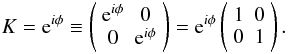
Noordam (1996), I can now introduce a scalar
K-Jones matrix representing the phase delay effect.
After all, phase delay is just another linear transformation of the signal, and is
perfectly amenable to the Jones formalism:
are the direction cosines of σ, and λ is
signal wavelength. It is customary to define u in units of
wavelength, which allows us to omit the λ-1 term. Following
Noordam (1996), I can now introduce a scalar
K-Jones matrix representing the phase delay effect.
After all, phase delay is just another linear transformation of the signal, and is
perfectly amenable to the Jones formalism: 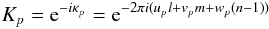 (10)The
RIME for a single uncorrupted point source is then simply:
(10)The
RIME for a single uncorrupted point source is then simply:  (11)Substituting
the exponents for Kp from Eq. (10), and remembering that scalar matrices
commute with everything, we can recast Eq. (11) in a more traditional form9:
(11)Substituting
the exponents for Kp from Eq. (10), and remembering that scalar matrices
commute with everything, we can recast Eq. (11) in a more traditional form9:
 (12)which expresses the
visibility as a function of baseline uvw
coordinates upq. I
shall call the visibility matrix given by Eqs. (11) or (12) the source
coherency, and write it as Xpq. In the traditional
view of radio interferometry, Xpq is a measurement of the
coherency function
(12)which expresses the
visibility as a function of baseline uvw
coordinates upq. I
shall call the visibility matrix given by Eqs. (11) or (12) the source
coherency, and write it as Xpq. In the traditional
view of radio interferometry, Xpq is a measurement of the
coherency function  at
point
upq,vpq,wpq
(with
at
point
upq,vpq,wpq
(with  being a 2 × 2
complex matrix rather than the traditional scalar complex function). For the purposes of
these papers, let us adopt an operational definition of source coherency
as being the visibility that would be measured by a corruption-free
interferometer. For a point source, the coherency is given by Eq. (11).
being a 2 × 2
complex matrix rather than the traditional scalar complex function). For the purposes of
these papers, let us adopt an operational definition of source coherency
as being the visibility that would be measured by a corruption-free
interferometer. For a point source, the coherency is given by Eq. (11).
1.8. A single corrupted point source
A real-world interferometer will have some “corrupting” effects in the signal path, in addition to the nominal phase delay Kp. Since the latter is scalar and thus commutes with everything, we can move it to the beginning of the Jones chain, and write the total Jones Jp of Eq. (8) as
 where
Gp represents all the other
(corrupting) effects. We can then formulate the RIME for a single corrupted point source
as:
where
Gp represents all the other
(corrupting) effects. We can then formulate the RIME for a single corrupted point source
as:  (13)where
Xpq is the source coherency, as defined above.
(13)where
Xpq is the source coherency, as defined above.
2. Multiple discrete sources
Let us now consider a sky composed of N point sources. The contributions
of each source to the measured visibility matrix Vpq add up
linearly. The signal propagation path is different for each source s and
antenna p, but each path can be described by its own Jones matrix
Jsp. Equation (8) then becomes:  (14)Remember that each
Jsp is a product of a
(generally non-commuting) Jones chain, corresponding to the physical order
of effects along the signal path:
(14)Remember that each
Jsp is a product of a
(generally non-commuting) Jones chain, corresponding to the physical order
of effects along the signal path:
 where effects
represented by the right side of the chain
(...Jsp1) occur
“at the source”, and effects on the left side of the chain
(Jspn...) “at
the antenna”. Somewhere along the chain is the phase term
Ksp, but since (being a scalar matrix) it
commutes with everything, we are free to move it to any position in the product.
where effects
represented by the right side of the chain
(...Jsp1) occur
“at the source”, and effects on the left side of the chain
(Jspn...) “at
the antenna”. Somewhere along the chain is the phase term
Ksp, but since (being a scalar matrix) it
commutes with everything, we are free to move it to any position in the product.
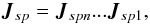
Some elements in the chain may be the same for all sources. This tends to be true for effects at the antenna end of the signal path, such as electronic gain. Let us then collapse the chain into a product of three Jones matrices:
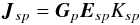 Gp
is the source-independent “antenna” (left) side of the Jones chain, i.e. the product of the
terms beginning with Jspn, up to
and not including the leftmost source-dependent term (if the entire chain is
source-dependent, Gp is simply
unity), Esp is the
source-dependent remainder of the chain, and
Ksp is the phase term. We can then recast
Eq. (14) as follows:
Gp
is the source-independent “antenna” (left) side of the Jones chain, i.e. the product of the
terms beginning with Jspn, up to
and not including the leftmost source-dependent term (if the entire chain is
source-dependent, Gp is simply
unity), Esp is the
source-dependent remainder of the chain, and
Ksp is the phase term. We can then recast
Eq. (14) as follows: 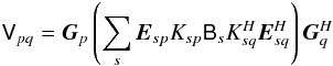 (15)Or,
using the source coherency of Eq. (11):
(15)Or,
using the source coherency of Eq. (11):
 (16)Gp
describes the direction-independent effects (DIEs), or the
uv-Jones terms, and
Esp the
direction-dependent effects (DDEs), or the sky-Jones
terms.
(16)Gp
describes the direction-independent effects (DIEs), or the
uv-Jones terms, and
Esp the
direction-dependent effects (DDEs), or the sky-Jones
terms.
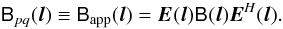
In principle, the sum in Eq. (16) should be taken over all sufficiently bright10 sources in the sky, but in practice our FoV is limited by the voltage beam pattern of each antenna, or by the horizon, in the case of an all-sky instrument such as the Low Frequency Array (LOFAR). In RIME terms, beam gain is just another Jones term in the chain, ensuring Esp → 0 for sources outside the beam.
If the observed field has little to none spatially extended emission, this form of the RIME is already powerful enough to allow for calibration of DDEs, as I shall show in Paper III (Smirnov 2011b).
3. The full-sky RIME
In the more general case, the sky is not a sum of discrete sources, but rather a continuous
brightness distribution  , where
σ is a (unit) direction vector. For each antenna
p, we then have a Jones term
Jp(σ),
describing the signal path for direction σ. To get the total
visibility as measured by an interferometer, we must integrate Eq. (8) over all possible directions, i.e. over a
unit sphere:
, where
σ is a (unit) direction vector. For each antenna
p, we then have a Jones term
Jp(σ),
describing the signal path for direction σ. To get the total
visibility as measured by an interferometer, we must integrate Eq. (8) over all possible directions, i.e. over a
unit sphere:
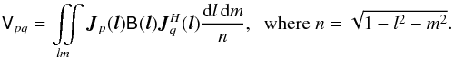
 This spherical integral is
not very tractable, so we perform a sine projection of the sphere onto the plane
(l,m) tangential at the field centre11. Note that this analysis is fully analogous to that of Thompson et al. (2001, Sect. 3.1), with only the integrand being somewhat
different. The integral then becomes:
This spherical integral is
not very tractable, so we perform a sine projection of the sphere onto the plane
(l,m) tangential at the field centre11. Note that this analysis is fully analogous to that of Thompson et al. (2001, Sect. 3.1), with only the integrand being somewhat
different. The integral then becomes:
 I’m going to use
l and (l,m) interchangeably from now on.
By analogy with Eq. (15), we now decompose
Jp(l)
into a direction-independent part G, a direction-dependent
part
I’m going to use
l and (l,m) interchangeably from now on.
By analogy with Eq. (15), we now decompose
Jp(l)
into a direction-independent part G, a direction-dependent
part  ,
and the phase term K:
,
and the phase term K:
 Substituting this
into the integral, and commuting the K terms around, we get
Substituting this
into the integral, and commuting the K terms around, we get 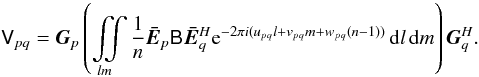 (17)This equation is one
form of a general full-sky RIME. It is in fact a type of three-dimensional Fourier
transform; the non-coplanarity term in the exponent,
wpq(n − 1), is what
prevents us from treating it as the much simpler 2D transform. Since
wpq = wp − wq,
we can decompose the non-coplanarity term into per-antenna terms
(17)This equation is one
form of a general full-sky RIME. It is in fact a type of three-dimensional Fourier
transform; the non-coplanarity term in the exponent,
wpq(n − 1), is what
prevents us from treating it as the much simpler 2D transform. Since
wpq = wp − wq,
we can decompose the non-coplanarity term into per-antenna terms
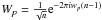 .
These can be thought of direction-dependent Jones matrices in their own right, and subsumed
into the overall sky-Jones term by defining
.
These can be thought of direction-dependent Jones matrices in their own right, and subsumed
into the overall sky-Jones term by defining  .
The full-sky RIME (Eq. (17)) can then be
rewritten using a 2D Fourier Transform of the apparent sky as seen by baseline
pq, or Bpq:
.
The full-sky RIME (Eq. (17)) can then be
rewritten using a 2D Fourier Transform of the apparent sky as seen by baseline
pq, or Bpq: 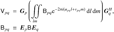 (18)I
shall return to this general formulation in Paper II (Smirnov 2011a). In the meantime, consider the import of those pq
indices in Bpq. They are telling us that we’re measuring a 2D
Fourier Transform of the sky – but the “sky” is different for every baseline! This violates
the fundamental premise of traditional selfcal, which assumes that we’re measuring the F.T.
of one common sky. From the above, it follows that this premise only holds when all DDEs are
identical across all antennas:
Ep(l) ≡ E(l)
(or at least where
(18)I
shall return to this general formulation in Paper II (Smirnov 2011a). In the meantime, consider the import of those pq
indices in Bpq. They are telling us that we’re measuring a 2D
Fourier Transform of the sky – but the “sky” is different for every baseline! This violates
the fundamental premise of traditional selfcal, which assumes that we’re measuring the F.T.
of one common sky. From the above, it follows that this premise only holds when all DDEs are
identical across all antennas:
Ep(l) ≡ E(l)
(or at least where  ). Only under this condition does
the apparent sky Bpq become the same on all baselines (in the
traditional view, this corresponds to the “true” sky attenuated by the power beam):
). Only under this condition does
the apparent sky Bpq become the same on all baselines (in the
traditional view, this corresponds to the “true” sky attenuated by the power beam):
 If this is met, we can then
rewrite the full-sky RIME as:
If this is met, we can then
rewrite the full-sky RIME as:  (19)where
 , and the
matrix function
, and the
matrix function  is simply
the (element-by-element) two-dimensional Fourier transform12 of the matrix function Bapp(l). I
shall also write this as
is simply
the (element-by-element) two-dimensional Fourier transform12 of the matrix function Bapp(l). I
shall also write this as  . The similarity to
Eq. (13) of a single point source is
readily apparent. For obvious reasons, I shall call the sky
coherency. Effectively, we have derived the van Cittert-Zernike theorem (VCZ),
the cornerstone of radio interferometry (Thompson et al.
2001, Sect. 14.1), from the basic RIME!
. The similarity to
Eq. (13) of a single point source is
readily apparent. For obvious reasons, I shall call the sky
coherency. Effectively, we have derived the van Cittert-Zernike theorem (VCZ),
the cornerstone of radio interferometry (Thompson et al.
2001, Sect. 14.1), from the basic RIME!
Such an approach turns the original original coherency matrix formulation of Hamaker (2000) on its head. Note that Eq. (19) here is the same as Eq. (2) of that work. In the RIME papers, Hamaker et al. defer to VCZ, treating the coherency as a “given” (while recasting it to matrix form) to which Jones matrices then apply. Treating phase (K) as a Jones matrix in its own right (Noordam 1996) allows for a natural extension of the Jones formalism into the (l,m) plane, and shows that VCZ is actually a consequence of the RIME rather than being something extrinsic to it. This also allows DDEs to be incorporated into the same formalism, in a manner similar to that suggested for w-projection (Cornwell et al. 2008). I shall return to this subject in Paper II (Smirnov 2011a).
3.1. Time variability and the fundamental assumption of selfcal
I have hitherto ignored the time variable. Signal propagation effects, and indeed the sky itself, do vary in time, but the RIME describes an effectively instantaneous measurement (ignoring for the moment the issue of time averaging, which will be considered separately in Sect. 5.2). Time begins to play a critical role when we consider DDEs.
At any point in time, an interferometer given by Eq. (19) measures the coherency function
at a
number of points upq (i.e. for
all baselines pq). This “snapshot” measurement gives a limited sampling
of the uv plane. To sample the uv plane more fully, we
usually rely on the Earth’s rotation, which over several hours effectively “swings” every
baseline vector upq through an
arc in the uv plane. Therefore, for Eq. (19) to hold throughout an observation, we must additionally assume
that the apparent sky Bapp remains constant over the observation time! In other
words, unless we’re dealing with snapshot imaging, the
Ep ≡ E
assumption must be further augmented:  (20)This equation captures
the fundamental assumption of traditional selfcal. I shall call DDEs that satisfy
Eq. (20) trivial DDEs.
As shown above, trivial DDEs effectively replace the true sky
by a single
apparent sky Bapp, and are not usually a problem for calibration, since they
can be corrected for entirely in the image plane13.
For example, the primary beam gain is usually treated as a trivial DDE in 2GC packages
(see Paper II, Smirnov 2011a, Sect. 2.1).
(20)This equation captures
the fundamental assumption of traditional selfcal. I shall call DDEs that satisfy
Eq. (20) trivial DDEs.
As shown above, trivial DDEs effectively replace the true sky
by a single
apparent sky Bapp, and are not usually a problem for calibration, since they
can be corrected for entirely in the image plane13.
For example, the primary beam gain is usually treated as a trivial DDE in 2GC packages
(see Paper II, Smirnov 2011a, Sect. 2.1).
Equation (20) is most readily met with narrow FoVs (i.e. with Ep rapidly going to zero away from the field centre, leaving little scope for other variations), small arrays (small wp, also all stations see through the same atmosphere), higher frequencies (narrow FoV, less ionospheric effects), and also with coplanar arrays such as the WSRT (wp ≡ 0, thus Wp ≡ 1). The new crop of instruments is, of course, trending in the opposite direction on all these points, and is thus subject to far more severe and non-trivial DDEs.
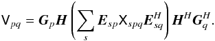
4. Matrix closures and singularities
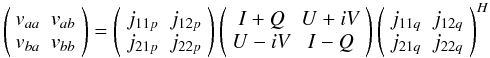
Scalar closure relationships have played an important role in 2GC calibration, both as a diagnostic tool, and as an observable. Traditionally, these are expressed in terms of a three-way phase closure and a four-way amplitude closure (see e.g. Thompson et al. 2001, Sect. 10.3). Since the underlying premise of a closure relationship is that observed scalar visibilities can be expressed in terms of per-antenna scalar gains, and the RIME is a generalization of the same premise in matrix terms, it seems worthwhile to see if a general matrix (i.e. fully polarimetric) closure relationship can be derived.
Indeed, in the case of a single point source, we can write out a four-way closure for
antennas m,n,p,q as follows:  (21)The above equation can
be easily verified by substituting in Eq. (8) for each visibility term, and remembering that
(21)The above equation can
be easily verified by substituting in Eq. (8) for each visibility term, and remembering that
 .
.
Since matrix inversion is involved, the essential requirement here is non-singularity of
all matrices in Eq. (8). The brightness
matrix is non-singular by
definition (unless it’s trivially zero), but what does it mean for a Jones matrix to be
singular? Some examples of singular matrices are:
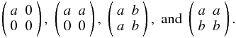 The physical meaning of a
singular Jones matrix can be grasped by substituting these into Eq. (2). The first two examples correspond to an
antenna measuring zero voltage on one of the receptors (e.g. a broken wire). The latter two
are examples of redundant measurements: both receptors will measure the same voltage, or
linearly dependent voltages (consider, e.g., a flat aperture array, with a source in the
plane of the dipoles). In all four cases there’s irrecoverable loss of polarization
information, so a polarization closure relation like Eq. (21) breaks down. (Note that the scalar analogue of this is simply a null
scalar visibility, in which case scalar closures also break down.)
The physical meaning of a
singular Jones matrix can be grasped by substituting these into Eq. (2). The first two examples correspond to an
antenna measuring zero voltage on one of the receptors (e.g. a broken wire). The latter two
are examples of redundant measurements: both receptors will measure the same voltage, or
linearly dependent voltages (consider, e.g., a flat aperture array, with a source in the
plane of the dipoles). In all four cases there’s irrecoverable loss of polarization
information, so a polarization closure relation like Eq. (21) breaks down. (Note that the scalar analogue of this is simply a null
scalar visibility, in which case scalar closures also break down.)
In the wide-field or all-sky case (Eq. (18)), simple closures (whether matrix or scalar) no longer apply. However, the
contribution of each discrete point source to the overall visibility is
still subject to a closure relationship. It is perhaps useful to formulate this in
differential terms. Consider a brightness distribution
 , and let
this correspond to a set of observed visibilities
, and let
this correspond to a set of observed visibilities  .
Adding a point source of flux B1 at position
l1 gives us the brightness distribution:
.
Adding a point source of flux B1 at position
l1 gives us the brightness distribution:
 where
δ is the Kronecker delta-function, with corresponding observed
visibilities
where
δ is the Kronecker delta-function, with corresponding observed
visibilities  .
From the RIME (and Eq. (18) in particular)
it then necessarily follows that the differential visibilities
.
From the RIME (and Eq. (18) in particular)
it then necessarily follows that the differential visibilities
 will then satisfy the matrix closure relationship of Eq. (21).
5. Limitations of the RIME formalism
5.1. Noise
The RIME as presented here and in the original papers is formulated for a noise-free measurement. In practice, each element of the Vpq matrix (i.e. each complex visibility) is accompanied by uncorrelated Gaussian noise in the real and imaginary parts; a detailed treatment of this can be found in Thompson et al. (2001, Sect. 6.2). The noise level imposes a hard sensitivity limit on any given observation, which has a few implications relevant to our purposes:
-
“Reaching the noise” has becomethe “gold standard” of calibration (seePaper II, Smirnov 2011a).Many reductions are limited by calibration artifacts rather thanthe noise.
-
Corrections to the data (however one defines the term) can potentially distort the noise level across an observation in complicated ways, so due care must be taken.
-
Faint sources below the noise threshold can be effectively ignored.
-
Numerical approximations can be considered “good enough” once they get to within the noise (assuming no systematic errors), but see Paper III (Smirnov 2011b, Sect. 2.6, Fig. 17) for a big caveat to this.
The latter two considerations are what I refer to by “sufficiently faint” sources and “sufficiently close” approximations throughout this series of papers.
5.2. Smearing and decoherence
In Sect. 1.3, when going from Eqs. (5) to (6), we assumed that the Jones matrix
Jp is constant over the
time/frequency bin of the correlator. That this is, strictly speaking, never actually the
case can be seen from the definition of the K-Jones term in Eq. (10). The vector
up is defined in units of
wavelength, making Kp variable in frequency.
The Earth’s rotation causes up
to rotate in our (fixed relative to the sky) coordinate frame, which also makes variable
in time. To take this into account, the RIME (in any form) should be rewritten as an
integration over a time/frequency interval. For example, the basic RIME of Eq. (8), when considering the integration bin
[t0,t1] × [ν0,ν1],
should be properly rewritten as:  (22)which
becomes Eq. (8) at the limit of
Δt,Δν → 0. Since J
contains K, the complex phase of which is variable in frequency and time,
the integration in Eq. (22) always results
in a net loss of amplitude in the measured ⟨ Vpq ⟩ . This
mechanism is well-known in classical interferometry, and is commonly called
time/bandwidth decorrelation or smearing. Note that a
phase variation in any other Jones term in the signal chain will have a similar effect.
The VLBI community knows of it in the guise of decoherence due to
atmospheric phase variations; in RIME terms, atmospheric decoherence is just Eq. (22) applied to ionospheric
Z-Jones or tropospheric T-Jones14. I shall use the term decoherence for the general
effect; and smearing for the specific case of decoherence caused by the
K term.
(22)which
becomes Eq. (8) at the limit of
Δt,Δν → 0. Since J
contains K, the complex phase of which is variable in frequency and time,
the integration in Eq. (22) always results
in a net loss of amplitude in the measured ⟨ Vpq ⟩ . This
mechanism is well-known in classical interferometry, and is commonly called
time/bandwidth decorrelation or smearing. Note that a
phase variation in any other Jones term in the signal chain will have a similar effect.
The VLBI community knows of it in the guise of decoherence due to
atmospheric phase variations; in RIME terms, atmospheric decoherence is just Eq. (22) applied to ionospheric
Z-Jones or tropospheric T-Jones14. I shall use the term decoherence for the general
effect; and smearing for the specific case of decoherence caused by the
K term.
The mathematics of smearing are well-known for the scalar case, see e.g. Thompson et al. (2001, Sect. 6.4) and Bridle & Schwab (1999). Smearing increases with baseline length (upq) and distance from phase center (l,m). Since the noise amplitude does not decrease, smearing results in a decrease of sensitivity. Hamaker et al. (1996) mention smearing in the context of the RIME. Since integration (and thus smearing) of a matrix equation is an element-by-element operation, treatment of smearing within the RIME formalism is a trivial extension of the scalar equations.
For the general case of decoherence, a useful first-order approximation can be obtained by assuming that Δt and Δν are small enough that the amplitude of Vpq remains constant, while the complex phase varies linearly. The relation
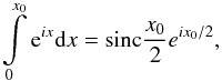 which is well-known
from the case of smearing with a square taper, then gives us an approximate equation for
decoherence, in terms of the phase changes in time (ΔΨ) and
frequency (ΔΦ):
which is well-known
from the case of smearing with a square taper, then gives us an approximate equation for
decoherence, in terms of the phase changes in time (ΔΨ) and
frequency (ΔΦ):  (23)Equation (23) is straightforward to apply numerically,
and is independent of the particular form of J responsible
for the decoherence. However, the assumption of linearity in phase over the time/frequency
bin can only hold for the visibility of a single source. In fact, it is easy to see that
any approximation treating decoherence as an amplitude-only effect can,
in principle, only apply on a source-by-source basis – just consider the case of smearing,
which varies significantly with distance from phase centre. In an equation like (16), the approximation can be applied to each
term in the sum individually, or at least to as many of the brightest sources as is
practical. This approach was used for the calibration described in Paper III (Smirnov 2011b).
(23)Equation (23) is straightforward to apply numerically,
and is independent of the particular form of J responsible
for the decoherence. However, the assumption of linearity in phase over the time/frequency
bin can only hold for the visibility of a single source. In fact, it is easy to see that
any approximation treating decoherence as an amplitude-only effect can,
in principle, only apply on a source-by-source basis – just consider the case of smearing,
which varies significantly with distance from phase centre. In an equation like (16), the approximation can be applied to each
term in the sum individually, or at least to as many of the brightest sources as is
practical. This approach was used for the calibration described in Paper III (Smirnov 2011b).
5.3. Interferometer-based errors
The term interferometer-based errors refers to measurement errors that
cannot be represented by per-antenna terms. These are also called closure
errors, since they violate the closure relationships of Sect. 4. When formulating Eq. (8), we assumed that the visibility matrix
Vpq output by the correlator is a perfect measurement of
correlations between antenna voltages. Closure errors represent additional baseline-based
effects. Assuming these are linear, and following Noordam
(1996), we could rewrite the full-sky RIME of Eq. (19) as: 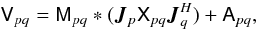 (24)where
Mpq is a 2 × 2 matrix of multiplicative interferometer
errors, Apq is a 2 × 2 matrix of additive errors, and “∗”
represents element-by-element (rather than matrix) multiplication.
(24)where
Mpq is a 2 × 2 matrix of multiplicative interferometer
errors, Apq is a 2 × 2 matrix of additive errors, and “∗”
represents element-by-element (rather than matrix) multiplication.
Given a model for Xpq, observed data
Vpq, and self-calibrated per-antenna terms
Jp, it is trivial to
estimate  and
and
 using Eq. (24). It is also trivial to see that the
equation is ill-conditioned: any model can be made to fit
the data by choosing suitable values for and
. We therefore need
to assume some additional constraints, such as closure errors being fixed (or only slowly
varying) in time and/or frequency.
using Eq. (24). It is also trivial to see that the
equation is ill-conditioned: any model can be made to fit
the data by choosing suitable values for and
. We therefore need
to assume some additional constraints, such as closure errors being fixed (or only slowly
varying) in time and/or frequency.
In practice, closure errors arise due to a combination of effects:
-
The traditional “purely instrumental” cause is the use of analogcomponents in the signal chain and parts of the correlator, which istypical of the previous generations of radio interferometers. Newtelescope designs tend to digitize the signal much closer to thereceiver, and use all-digital correlators, presumably eliminatinginstrumental closure errors.
-
Smearing and decoherence (Sect. 5.2) is a baseline-based effect, and will thus manifest itself as a closure errors, unless it is properly taken into account in the model for Xpq.
-
In general, any source structure or flux not represented by the model Xpq will also show up as a closure error.
A solution for and/or
will tend to
subsume all these effects. This is dangerous, as it can actually attenuate sources in the
final images, as illustrated in Paper III (Smirnov
2011b, Sect. 1.5). One must thus be very conservative with closure error
solutions, lest they become just another “fudge factor” in the equations.
5.4. A three-dimensional RIME?
Recent work by Carozzi & Woan (2009) highlights a limitation of the 2 × 2 Jones formalism. They point out that since we’re measuring a 3D brightness distribution, the radiation from off-center sources is only approximately paraxial (equivalently, the EM waves are only approximately transverse). From this it follows that a 2D description of the EMF based on a rank-2 vector (the e used above) is insufficient, and a rank-3 formalism is proposed.
The main implication of the Carozzi-Woan result for the 2 × 2 formalism is that the
latter is still valid in general (at least for dual-receptor arrays), but the full-sky
RIME of Eq. (17) must be augmented with an
additional direction-dependent Jones term called the xy-projected
transformation matrix, designated as  (see their Eq. (34)), which corresponds to a projection of the 3D brightness distribution
onto the plane of the receptors. If all the receptors of the array are plane-parallel
(Carozzi & Woan call this a plane-polarized interferometer),
is a trivial DDE (in the sense of Eq. (20)), manifesting itself as a polarization aberration that increases with
l,m (see their Fig. 2). For non-parallel receptors,
should be a non-trivial DDE!
(see their Eq. (34)), which corresponds to a projection of the 3D brightness distribution
onto the plane of the receptors. If all the receptors of the array are plane-parallel
(Carozzi & Woan call this a plane-polarized interferometer),
is a trivial DDE (in the sense of Eq. (20)), manifesting itself as a polarization aberration that increases with
l,m (see their Fig. 2). For non-parallel receptors,
should be a non-trivial DDE!
Classical dish arrays are plane-polarized by design, but deviate from this in practice due to pointing errors and other misalignments. The resulting effect is expected to be tiny given the typically narrow FoV of a dish, but it would be intriguing to see whether it can be detected in deliberately mispointed WSRT observations, given the extremely high dynamic range routinely achieved at the WSRT. On the other hand, an aperture array such as LOFAR should show a far more significant deviation from the plane-polarized case (due to the curvature of the Earth, as well as the all-sky FoV). With LOFAR’s (as yet) relatively low dynamic range and extreme instrumental polarization, the effect may be challenging to detect at present. Further work on the subject is urgently required, given the polarization purity requirements of future telescopes (and in particular the SKA).
6. Alternative formulations
6.1. Mueller vs. Jones formalism
The original paper by Hamaker et al. (1996) formulated the RIME in terms of 4 × 4 Mueller matrices (Mueller 1948). This is mathematically fully equivalent to the 2 × 2 form introduced by Hamaker (2000) in the fourth paper, and has since been adopted by many authors (Noordam 1996; Thompson et al. 2001; Bhatnagar et al. 2008; Rau et al. 2009). In my view, this is somewhat unfortunate, as the 2 × 2 formulation is both simpler and more elegant, and has far more intuitive appeal, especially for understanding calibration problems. For completeness, I will make an explicit link to the 4 × 4 form here.
Instead of taking the matrix product of two voltage vectors
vp and
vq and getting a 2 × 2
visibility matrix, as in Eq. (4), we can
take the outer product of the two to get the visibility
vector vpq:
 Combining
this with Eq. (2), we get
Combining
this with Eq. (2), we get
 which
then gives us the 4 × 4 form of Eq. (8):
which
then gives us the 4 × 4 form of Eq. (8):
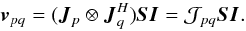 (25)Here,
 is a 4 × 4 matrix describing the combined effect of the signal paths to antennas
p and q, I is a column
vector of the Stokes parameters (I,Q,U,V), and
S is a conversion matrix that turns the Stokes vector into
the brightness vector15:
is a 4 × 4 matrix describing the combined effect of the signal paths to antennas
p and q, I is a column
vector of the Stokes parameters (I,Q,U,V), and
S is a conversion matrix that turns the Stokes vector into
the brightness vector15:
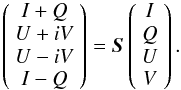 The
equivalent of the “onion” form of Eq. (9)
is then:
The
equivalent of the “onion” form of Eq. (9)
is then:  (26)Likewise, the
full-sky RIME of Eq. (18) can be written
in the 4 × 4 form as:
(26)Likewise, the
full-sky RIME of Eq. (18) can be written
in the 4 × 4 form as: 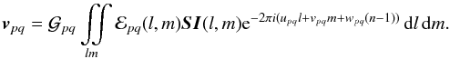 (27)This form of the
RIME is particularly favoured when describing imaging problems (Bhatnagar et al. 2008; Rau et al.
2009). It emphasizes that an interferometer performs a linear operation on the
sky distribution I(l,m), via the linear
operators
(27)This form of the
RIME is particularly favoured when describing imaging problems (Bhatnagar et al. 2008; Rau et al.
2009). It emphasizes that an interferometer performs a linear operation on the
sky distribution I(l,m), via the linear
operators  ,
ℰpq(l,m), and the Fourier Transform ℱ,
while eliding the internal structure of
,
ℰpq(l,m), and the Fourier Transform ℱ,
while eliding the internal structure of  and ℰ.
On the other hand, if we’re interested in the underlying physics of signal propagation (as is often the case for calibration problems), then the 4 × 4 form of the RIME becomes extremely opaque. When considering any specific set of propagation effects (and its corresponding Jones chain), the outer product operation turns simple-looking 2 × 2 Jones matrices into an intractable sea of indices; see Bhatnagar et al. (2008, Eq. (4)) and Hamaker et al. (1996, Appendix A) for typical examples. The 2 × 2 form provides a more transparent description of calibration problems, and for this reason is also far better suited to teaching the RIME. An excellent example of this transparency is given in Paper II (Smirnov 2011a, Sect. 2.2.2), where I consider the effect of differential Faraday rotation.
There are also potential computational issues raised by the 4 × 4 formalism. A naive implementation of, e.g., Eq. (26) incurs a series of 4 × 4 matrix multiplications for each interferometer and time/frequency point. Multiplication of two 4 × 4 matrices costs 112 floating-point operations (flops), and the outer product operation another 16. Therefore, each pair of Jones terms in the chain incurs 128 flops. The same equation in 2 × 2 form invokes 12 floating-point operations (flops) per matrix multiplication, or 24 per each pair of Jones terms. This is roughly 5 times fewer than the 4 × 4 case.
Often, the true computational bottleneck lies elsewhere, i.e. in solving (for calibration) or gridding (for imaging), in which case these considerations are irrelevant. However, when running massive simulations (that is, using the RIME to predict visibilities), my profiling of MeqTrees has often shown matrix multiplication to be the major consumer of CPU time. In this case, implementing calculations using the 2 × 2 form represents a significant optimization.
6.2. Jones-specific formulations
Formulations of the RIME such as Eqs. (18) or (16) are entirely general
and non-specific, in the sense that they allow for any combination of propagation effects
to be inserted in place of the G and
E terms. A specific formulation may be obtained by
inserting a particular sequence of Jones matrices. The first RIME paper (Hamaker et al. 1996) already suggested a specific Jones
chain. This was further elaborated on by Noordam
(1996), and eventually implemented in AIPS++, which subsequently became CASA. The
Jones chain used by current versions of CASA is described by Myers et al. (2010, Appendix E.1):  (28)The Jones matrices
given here correspond to particular effects in the signal chain, with specific
parameterizations (e.g. Bp is a
frequency-variable bandpass, Gp
is time-variable receiver gain, etc.). Other authors (Rau
et al. 2009) suggest variations on this theme.
(28)The Jones matrices
given here correspond to particular effects in the signal chain, with specific
parameterizations (e.g. Bp is a
frequency-variable bandpass, Gp
is time-variable receiver gain, etc.). Other authors (Rau
et al. 2009) suggest variations on this theme.
Such a “Jones-specific” approach has considerable merit, in that it shows how different real-life propagation effects fit together, and gives us something specific to be thought about and implemented in software. It does have a few pitfalls which should be pointed out.
The first pitfall of this approach is that it tends to place the trees firmly before the forest. A major virtue of the RIME is its elegance and simplicity, but this gets obscured as soon as elaborate chains of Jones matrices are written out. I submit that the RIME’s slow acceptance among astronomers at large is, in some part, due to the literature being full of equations similar to (28). That they are just specific cases of what is at core a very simple and elegant equation is a point perhaps so obvious that some authors do not bother noting it, but it cannot be stressed enough!
The second pitfall is that an equation like (28), when implemented in software, can be both too specific, and insufficiently flexible. (Note that the CASA implementation specifies both the time/frequency behaviour, and the form of the Jones terms, e.g. G is diagonal and variable in time, B is diagonal and variable in frequency, D has a specific “leakage” form, etc). For instance, the calibration described in Paper III (Smirnov 2011b) cannot be done in CASA, despite using an ostensibly much simpler form of the RIME, because it includes a Jones term that was not anticipated in the CASA design. A second major virtue of the RIME is its ability to describe different propagation effects; this is immediately compromised if only a specific and limited set of these is chosen for implementation.
A final pitfall of the Jones-specific view is that it tends to stereotype approaches to calibration. Equation (28) is a huge improvement on the ad hoc approaches of older software systems, but in the end it is just some model of an interferometer that happens to work well enough for “classically-designed” instruments such as the VLA and WSRT, in their most common regimes. It is not universally true that polarization effects can be completely described by a direction-independent leakage matrix (Dp), or bandpass by Bp – it just happens to be a practical first-order model, which completely breaks down for a new instrument such as LOFAR, where e.g. “leakage” is strongly direction-dependent. In fact, even WSRT results can be improved by departing from this model, as Paper III (Smirnov 2011b) will show. We must therefore take care that our thinking about calibration does not fall into a rut marked out by a specific series of Jones terms.
6.3. Circular vs. linear polarizations
In Sect. 1, I mentioned that the RIME holds in any coordinate system. Hamaker et al. (1996) briefly discussed coordinate transforms in this context, but a few additional words on the subject are required.
Field vectors e and Jones matrices
J may be represented (by a particular set of complex
values) in any coordinate system, by picking a pair of complex basis vectors in the plane
orthogonal to the direction of propagation. I have used an orthonormal xy
system until now. Another useful system is that of circular polarization coordinates
rl, whose basis vectors (represented in the xy system)
are  and
and
 . Any other pair of basis
vectors may of course be used. In general, for any two coordinate systems S and T, there
will be a corresponding 2 × 2 conversion matrix
T, such that
eT = TeS,
where eS and
eT represent the same vector in the S and T
coordinate systems. Likewise, the representation of the linear operator
J transforms as
. Any other pair of basis
vectors may of course be used. In general, for any two coordinate systems S and T, there
will be a corresponding 2 × 2 conversion matrix
T, such that
eT = TeS,
where eS and
eT represent the same vector in the S and T
coordinate systems. Likewise, the representation of the linear operator
J transforms as  ,
while the brightness matrix (or indeed any
coherency matrix) transforms as
,
while the brightness matrix (or indeed any
coherency matrix) transforms as  Of
particular importance is the matrix for conversion from linear to circularly polarized
coordinates. This matrix is commonly designated as H (being
the mathematical equivalent of an electronic hybrid sometimes found in
antenna receivers):
Of
particular importance is the matrix for conversion from linear to circularly polarized
coordinates. This matrix is commonly designated as H (being
the mathematical equivalent of an electronic hybrid sometimes found in
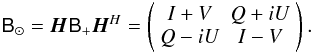
antenna receivers):  Consequently,
the brightness matrix , when represented
in circular polarization coordinates, has the following form (I’ll use the indices “⊙”
and “+” where necessary to disambiguate between circular and linear representations):
Consequently,
the brightness matrix , when represented
in circular polarization coordinates, has the following form (I’ll use the indices “⊙”
and “+” where necessary to disambiguate between circular and linear representations):
 While
EMF vectors and Jones matrices may be represented using an arbitrary basis, the receptor
voltages we actually measure are specific numbers. The voltage measurement process thus
implies a preferred coordinate system, i.e. circular for circular
receptors, and linear for linear receptors.
While
EMF vectors and Jones matrices may be represented using an arbitrary basis, the receptor
voltages we actually measure are specific numbers. The voltage measurement process thus
implies a preferred coordinate system, i.e. circular for circular
receptors, and linear for linear receptors.
It is of course possible to convert measured data into a different coordinate frame after
the fact. It is also perfectly possible, and indeed may be desirable, to mix coordinate
systems within the RIME, by inserting appropriate coordinate conversion matrices into the
Jones chain. A commonly encountered assumption is that a “VLA RIME” must be written down
in circular coordinates and a “WSRT RIME” in linear, but this is by no means a fundamental
requirement! We’re free to express part of the signal propagation chain in one coordinate
frame, then insert conversion matrices at the appropriate place in the equation to switch
to a different coordinate frame. In the onion form of the RIME (Eq. (9)), this corresponds to a change of
coordinate systems as we go from one layer of the onion to another. For example:
 One
reason to consider the use of mixed coordinate systems is the opportunity to optimize the
representation of particular physical effects. As an example, a rotation in the
xy frame (e.g. ionospheric Faraday rotation, or parallactic angle) is
represented by a diagonal matrix in the rl frame. If the observed field
has no intrinsic linear polarization, the B⊙ matrix is also diagonal. If a
part of the RIME is known to contain diagonal matrices only, their product can be
evaluated with significant computational savings (compared to the full 2 × 2 matrix
regime). On the other hand, if the instrument is using linear receptors, then receiver
gains (G) should be expressed in the linear frame, lest
calibrating them become extremely awkward. We should therefore implement the RIME somewhat
like the above equation, with the appropriate H matrices
inserted as “late” in the chain as possible, so that only the minimum amount of
computation is done for the full 2 × 2 case. This approach is not yet exploited by any
existing software, but perhaps it should be. In particular, the MeqTrees system (Noordam & Smirnov 2010) automatically optimizes
internal calculations when only diagonal matrices are in play, and would provide a
suitable vehicle for exploring this technique.
One
reason to consider the use of mixed coordinate systems is the opportunity to optimize the
representation of particular physical effects. As an example, a rotation in the
xy frame (e.g. ionospheric Faraday rotation, or parallactic angle) is
represented by a diagonal matrix in the rl frame. If the observed field
has no intrinsic linear polarization, the B⊙ matrix is also diagonal. If a
part of the RIME is known to contain diagonal matrices only, their product can be
evaluated with significant computational savings (compared to the full 2 × 2 matrix
regime). On the other hand, if the instrument is using linear receptors, then receiver
gains (G) should be expressed in the linear frame, lest
calibrating them become extremely awkward. We should therefore implement the RIME somewhat
like the above equation, with the appropriate H matrices
inserted as “late” in the chain as possible, so that only the minimum amount of
computation is done for the full 2 × 2 case. This approach is not yet exploited by any
existing software, but perhaps it should be. In particular, the MeqTrees system (Noordam & Smirnov 2010) automatically optimizes
internal calculations when only diagonal matrices are in play, and would provide a
suitable vehicle for exploring this technique.
Note that the configuration matrix C proposed by Hamaker et al. (1996), and further discussed by Noordam (1996), plays a similar role, in that it converts from “antenna frame” to “voltage frame”. Here I simply suggest a generalization of this line of thinking. The RIME allows for an arbitrary mix of coordinate frames, as long as the appropriate conversion matrices are inserted in their rightful places16.
7. Errors and controversies
For all its elegance, even the simplest version of the RIME (e.g. as formulated in
Sect. 1.3) contains two points of confusion and
controversy. The first has to do with the sign of the iV term, and the
second with the factors of 2 in the definition of Vpq and
.
7.1. Sign of Stokes V
The sign of Stokes V has been a perennial source of confusion. The IAU (1973) definition specifies that V is positive for right-hand circular polarization, but the literature is littered with papers adopting the opposite convention. Fortunately, major software packages such as AIPS and MIRIAD follow the IAU definition (though this has not always been the case for their early versions). As for the iV term in the RIME, Papers I and II of the original series (Hamaker et al. 1996; Sault et al. 1996) used the sign convention of Eq. (7). In Paper III of the series, Hamaker & Bregman (1996) then discussed the issue in detail, and showed that this convention is “correct” in the sense of following from the IAU definitions for Stokes V and standard coordinate systems. However, in Paper IV, Hamaker (2000) then used the opposite sign convention! In Paper V, Hamaker (2006) noted the inconsistency, yet persisted in using the opposite convention.
For this series, I adopt the correct sign convention of the original RIME Papers I through III, as per Eq. (7).
In practice, few radio astronomers concern themselves with circular polarisation, which is perhaps why the confusion has been allowed to fester. Unfortunately, this also means that in the rare cases when sign of V is important, it must be fastidiously checked each time!
7.2. Factors of 2, or what is the unit response of an ideal interferometer?
A far more insidious issue is the factor of 2 in Eqs. (4) and (7). This has
been the subject of a long-standing controversy both in the literature and in software.
The definition of Stokes I in terms of the complex amplitudes of the
electric field is quite unambiguous (Thompson et al.
2001; Born & Wolf 1964). In
particular:  This
implies that a unit source of
I = 1,Q = U = V = 0
corresponds to complex amplitudes of
⟨ |ex|2 ⟩ = ⟨ |ey|2 ⟩ = 1/2.
What is less clear is how to relate this to the outputs of a correlator. That is, given an
ideal interferometer and a unit source at the phase centre, what visibility matrix
Vpq should we expect to see? (In other words, what is the
gain factor of an ideal interferometer?) This is something for which no unambiguous
definition exists. Historically, two conventions have emerged:
This
implies that a unit source of
I = 1,Q = U = V = 0
corresponds to complex amplitudes of
⟨ |ex|2 ⟩ = ⟨ |ey|2 ⟩ = 1/2.
What is less clear is how to relate this to the outputs of a correlator. That is, given an
ideal interferometer and a unit source at the phase centre, what visibility matrix
Vpq should we expect to see? (In other words, what is the
gain factor of an ideal interferometer?) This is something for which no unambiguous
definition exists. Historically, two conventions have emerged:
Convention-1/2.
Unity correlations correspond to unity complex amplitudes, so a 1 Jy source produces
correlations of 1/2 each: 
Convention-1.
Unity correlations correspond to unity Stokes I:
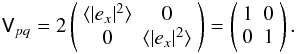 Convention-1/2
is somewhat more pleasing to the purists, as it retains standard physical units for
visibilities. This is the convention used throughout the RIME papers, beginning with
Hamaker et al. (1996), and also originally
adopted in the MeqTrees system (Noordam &
Smirnov 2010). However, Convention-1 is by far the more widespread, having been
adopted by AIPS and other software systems, which has caused it to become entrenched in
the minds of most radio astronomers.
Convention-1/2
is somewhat more pleasing to the purists, as it retains standard physical units for
visibilities. This is the convention used throughout the RIME papers, beginning with
Hamaker et al. (1996), and also originally
adopted in the MeqTrees system (Noordam &
Smirnov 2010). However, Convention-1 is by far the more widespread, having been
adopted by AIPS and other software systems, which has caused it to become entrenched in
the minds of most radio astronomers.
The first edition of what is effectively the main reference work of radio interferometry, Thompson et al. (1986), had a factor of 1/2 in the equations for interferometer response (Eq. (4.46)), but omitted it in Table 4.47. (I conjecture that this table may in fact be the origin of Convention-1!) By the time of the second edition, Convention-1 was already widespread, and the authors responded by dropping the factor of 1/2 after Eq. (4.29), noting that it was “omitted and considered to be subsumed within the overall gain factor.” (Thompson et al. 2001, see p. 102). For better or for worse, this has irrevocably consecrated Convention-1 as the one to follow.
Ultimately, flux scales are tied to known calibrator sources, whose brightnesses are quite unambiguously defined in units of janskys. This means that in practice, the factor of 2 is indeed quietly subsumed into the gain calibration. Problems arise when data is moved between software packages that follow different conventions. For example, data calibrated with MeqTrees (formerly using Convention-1/2) is kept in a Measurement Set (MS), yet the only tool available for making images from an MS is the AIPS++/CASA imager (Convention-1). This has often resulted in images with fluxes that were off by a factor of 2, so the MeqTrees project has recently switched to Convention-1.
In this paper, I have taken the difficult decision of breaking with the original
formulations, and recasting the RIME using Convention-1. There remains the question of
where to inject the requisite factor of 2. I have decided to do it “on the inside”, by
dropping the factor of 1/2 from the Hamaker (2000)
definition of the brightness matrix (Eq. (7)). The alternative was to add a factor of
2 to the “outside” of the equation. The “inside” approach appears to have a number of
practical advantages:
-
becomes
unity for a unit (1 Jy unpolarized) source.
-
The coherency of a point source at the phase centre (Sect. 1.7) becomes equivalent to its brightness (and not one-half of its brightness).
-
In the “onion” form of the ME (Eq. (9)), each successive layer of the onion corresponds to measurable visibilities, without needing to carry an explicit factor of 2 around.
8. Conclusions
Since its original formulation by Hamaker et al. (1996), the radio interferometer measurement equation (RIME) has provided the mathematical underpinnings for novel calibration methods and algorithms. Besides its explanatory power, the RIME formalism can be wonderfully simple and intuitive; this fact has become somewhat obscured by the many different directions that it has been taken in. Several authors have developed approaches to the DDE problem based on the RIME, using different (but mathematically equivalent) versions of the formalism. This paper has attempted to reformulate these using one consistent 2 × 2 formalism, in preparation for follow-up papers (II and III) that will put it to work. Finally, a number of misunderstandings and controversies has inevitably accrued themselves to the RIME over the years. Some of these have been addressed here. It is hoped that this paper has gone some way to making the RIME simple again.
All 2GC packages do use some specific and limited form of the RIME implicitly. This will be discussed further in Paper II (Smirnov 2011a).
This (admittedly subjective) judgment is firmly based on personal experience of teaching the RIME.
Hamaker (2000) calls Vpq the coherency matrix, in order to distinguish it from traditional scalar visibilities. Since the elements of the matrix are precisely the complex visibilities, I submit visibility matrix as a more logical term.
This is a crucial assumption, which I will revisit in Sect. 5.2.
Following a long-standing controversy, I have decided to break with Hamaker (2000) by omitting
 from the
definition of , and adding a
factor 2 to the definition of Vpq in Eq. (4). The reasons for this will be spelled out in
Sect. 7.2.
from the
definition of , and adding a
factor 2 to the definition of Vpq in Eq. (4). The reasons for this will be spelled out in
Sect. 7.2.
Note that this is only true for 2 × 2 matrices. Higher-order rotations do not commute.
As noted above, rotation can become diagonality through change of coordinate basis, so this doesn’t actually add anything to our general rule.
Note that there is some unfortunate confusion in coordinate systems used in radio interferometry. The IAU (1973) defines Stokes parameters in a right-handed coordinate system with x and y in the plane of the sky towards North and East, and the z axis pointing towards the observer. The conventional lm frame has l pointing East and m North. In practice, this means that rotation through parallactic angle must be applied in one direction in the lm frame, and in the opposite direction in the polarization frame. The formulations of the present paper are not affected.
The sign of the exponent in these equations is a matter of convention, and is therefore subject to perennial confusion. WSRT software uses “−”, but has used “+” in the past. VLA software seems to use “+”. Fortunately, in practice it is usually easy to tell which convention is being used, and conjugate the visibilities if needed.
Brighter than the noise, that is – see Sect. 5.1.
Or the pole, for East-West arrays, which does not materially change any of the arguments.
Note that I’m using u as a shorthand for both (u,v) and (u,v,w), depending on context.
Even then things are not always easy. Rapid variation in frequency, such as the 17 MHz “ripple” of the WSRT primary beam (see Paper II, Smirnov 2011a, Sect. 2.1.1) can cause considerable difficulty for spectral line calibration, even if the DDE is trivial in the sense of Eq. (20).
Small interferometers see very little atmospheric decoherence: if
Zp ≈ Zq
(as is the case for closely located stations), then
 , so
there is no net phase contribution to the integrand of Eq. (22).
, so
there is no net phase contribution to the integrand of Eq. (22).
A Mueller matrix represents a linear operation on Stokes vectors, and so does not
explicitly appear in these equations. For Eq. (25), the equivalent Mueller matrix is  .
.
Nor should we restrict our thinking to just the xy and rl frames. It could well be that the RIME of a future instrument will turn out to have a particularly elegant form in some other coordinate basis.
References
- Bhatnagar, S. 2009, in ASP Conf. Ser. 407, ed. D. J. Saikia, D. A. Green, Y. Gupta, & T. Venturi, 375 [Google Scholar]
- Bhatnagar, S., Cornwell, T. J., Golap, K., & Uson, J. M. 2008, A&A, 487, 419 [NASA ADS] [CrossRef] [EDP Sciences] [Google Scholar]
- Born, M., & Wolf, E. 1964, Principles of Optics (Pergamon Press) [Google Scholar]
- Bridle, A. H., & Schwab, F. R. 1999, in Synthesis Imaging in Radio Astronomy II, ed. G. B. Taylor, C. L. Carilli, & R. A. Perley, ASP Conf. Ser., 180, 371 [Google Scholar]
- Carozzi, T. D., & Woan, G. 2009, MNRAS, 395, 1558 [NASA ADS] [CrossRef] [Google Scholar]
- Cornwell, T. J., & Wilkinson, P. N. 1981, MNRAS, 196, 1067 [NASA ADS] [Google Scholar]
- Cornwell, T. J., Golap, K., & Bhatnagar, S. 2008, IEEE J. Selected Topics in Signal Process., 2, 647, 2 [NASA ADS] [CrossRef] [Google Scholar]
- Hamaker, J. P. 2000, A&AS, 143, 515 [NASA ADS] [CrossRef] [EDP Sciences] [Google Scholar]
- Hamaker, J. P. 2006, A&A, 456, 395 [NASA ADS] [CrossRef] [EDP Sciences] [Google Scholar]
- Hamaker, J. P., & Bregman, J. D. 1996, A&AS, 117, 161 [NASA ADS] [CrossRef] [EDP Sciences] [Google Scholar]
- Hamaker, J. P., Bregman, J. D., & Sault, R. J. 1996, A&AS, 117, 137 [NASA ADS] [CrossRef] [EDP Sciences] [Google Scholar]
- IAU 1973, Trans. IAU, 15b, 166 [Google Scholar]
- Jones, R. C. 1941, J. Opt. Soc. Amer., 31, 488 [Google Scholar]
- Mueller, H. 1948, J. Opt. Soc. Amer., 38, 661 [Google Scholar]
- Myers, S. T., Ott, J., & Elias, N. 2010, CASA Synthesis & Single Dish Reduction Cookbook, Release 3.0.1 [Google Scholar]
- Noordam, J. E. 1996, The Measurement Equation of a Generic Radio Telescope, Tech. rep., AIPS++ Note, 185 [Google Scholar]
- Noordam, J. E., & Smirnov, O. M. 2010, A&A, 524, A61 [NASA ADS] [CrossRef] [EDP Sciences] [Google Scholar]
- Rau, U., Bhatnagar, S., Voronkov, M. A., & Cornwell, T. J. 2009, IEEE Proc., 97, 1472 [Google Scholar]
- Sault, R. J., Hamaker, J. P., & Bregman, J. D. 1996, A&AS, 117, 149 [NASA ADS] [CrossRef] [EDP Sciences] [Google Scholar]
- Schilizzi, R. T. 2004, in SPIE Conf. Ser. 5489, ed. J. M. Oschmann, Jr., 62 [Google Scholar]
- Smirnov, O. M. 2011a, A&A, 527, A107 [NASA ADS] [CrossRef] [EDP Sciences] [Google Scholar]
- Smirnov, O. M. 2011b, A&A, 527, A108 [NASA ADS] [CrossRef] [EDP Sciences] [Google Scholar]
- Thompson, A. R., Moran, J. M., & Swenson, Jr., G. W. 1986, Interferometry and Synthesis in Radio Astronomy (New York: Wiley) [Google Scholar]
- Thompson, A. R., Moran, J. M., & Swenson, Jr., G. W. 2001, Interferometry and Synthesis in Radio Astronomy, 2nd Ed. (New York: Wiley) [Google Scholar]
Current usage metrics show cumulative count of Article Views (full-text article views including HTML views, PDF and ePub downloads, according to the available data) and Abstracts Views on Vision4Press platform.
Data correspond to usage on the plateform after 2015. The current usage metrics is available 48-96 hours after online publication and is updated daily on week days.
Initial download of the metrics may take a while.