| Issue |
A&A
Volume 527, March 2011
|
|
|---|---|---|
| Article Number | L4 | |
| Number of page(s) | 4 | |
| Section | Letters | |
| DOI | https://doi.org/10.1051/0004-6361/201015980 | |
| Published online | 31 January 2011 | |
Letter to the Editor
Twelve-hour spikes from the Crab Pevatron
1
INTEGRAL Science Data Centre, Université de Genève,
Chemin d’Ecogia 16,
1290
Versoix,
Switzerland
e-mail: This email address is being protected from spambots. You need JavaScript enabled to view it.
2
Observatoire de Genève, Université de Genève,
Chemin des Maillettes
51, 1290
Sauverny,
Switzerland
3
Institut für Astronomie und Astrophysik, Universität Tübingen,
Sand 1,
72076
Tübingen,
Germany
Received:
22
October
2010
Accepted:
15
December
2010
Abstract
Aims. The Crab nebula displayed a large γ-ray flare on September 18, 2010. To more closely understand the origin of this phenomenon, we analyze the INTEGRAL (20–500 keV) and Fermi (0.1–300 GeV) data collected almost simultaneously during the flare.
Methods. We divide the available data into three different sets, corresponding to the pre-flare period, the flare, and the subsequent quiescence. For each period, we perform timing and spectral analyses to differentiate between the contributions of the pulsar and the surrounding nebula to the γ-ray luminosity.
Results. No significant variations in the pulse profile and spectral characteristics are detected in the hard X-ray domain. In contrast, we identify three separate enhancements in the γ-ray flux lasting for about 12 h and separated by an interval of about two days from each other. The spectral analysis shows that the flux enhancement, confined below ~1 GeV, can be modelled by a power-law with a high energy exponential cut-off, where either the cut-off energy or the model normalization increased by a factor of ~5 relative to the pre-flare emission. We also confirm that the γ-ray flare is not pulsed.
Conclusions. The timing and spectral analysis indicate that the γ-ray flare is due to synchrotron emission from a very compact Pevatron located in the region of interaction between the pulsar wind and the surrounding nebula. These are the highest electron energies ever measured in a cosmic accelerator. The spectral properties of the flare are interpreted in the framework of a relativistically moving emitter and/or a harder emitting electron population.
Key words: acceleration of particles / astroparticle physics / magnetic fields / pulsars: individual: Crab / gamma rays: stars / X-rays: stars
© ESO, 2011
1. Introduction
With an integrated luminosity of about 5 × 1038 erg s-1 and a distance of ~2 kpc, the Crab supernova remnant is very bright from the radio domain to TeV energies (see e.g., Hester 2008, for a review). It is powered by a pulsar spinning on its axis in about 33 ms that injects energetic electrons into the surrounding nebula. Nearly all the nebular emission up to 0.4 GeV is believed to be produced by synchrotron cooling of these electrons in an average magnetic field of ~300 μG. At higher energies, inverse Compton (IC) cooling dominates.
The integrated high-energy flux of the nebula and the pulsar has been remarkably stable over the past few decades and the object is indeed used as a calibration source in several experiments (but see Wilson-Hodge et al. 2011,for the first report of a secular X-ray trend). On 2010 September 22 the AGILE collaboration (Tavani et al. 2010) reported the first γ-ray flare from a source positionally consistent with the Crab, during which the flux above 100 MeV was nearly double its normal value. The γ-ray flare from the direction of the Crab was confirmed by the Fermi collaboration (Buehler et al. 2010).
During a period partially covering the γ-ray flare, the Crab region was observed by the INTEGRAL satellite and the Swift/BAT telescope during its routine sky survey. No statistically significant increase in the Crab flux was observed in the IBIS/ISGRI light curves between 20 and 400 keV, as well as in the Swift/BAT 15 − 50 keV flux at a level of 5% at the 1σ confidence level (Ferrigno et al. 2010; Markwardt et al. 2010).
Swift/XRT observed the Crab region for 1 ks on 2010 September 22 at 16:42 UT and did not reveal any significant variation in the source flux, spectrum, and pulse profile (Evangelista et al. 2010). The ultraviolet and soft X-ray images excluded the presence of any bright unknown field object that could have contributed to the γ-ray flux (Heinke 2010). The near-infrared Crab flux in the J and H bands was also constant (Kanbach et al. 2010). Dedicated pointing performed by RXTE did not show any significant change in the overall spectral properties in the 3–20 keV band (Shaposhnikov et al. 2010).
A 5 ks TOO Chandra observation was performed on 2010 September 28 to monitor the morphology of the inner nebula. There are no particular variations with respect to the over 35 previous observations, with the possible exception of an anomalous extension of a bright knot closer (down to 3′′) to the pulsar, also noticed in one archival observation (Tennant et al. 2010). A subsequent HST optical observation of the Crab confirmed an increase in the emission about 3 arcsec south-east of the pulsar with respect to archival observations (Caraveo et al. 2010). However, it remains unclear whether this feature is related to the γ-ray event. The Crabγ-ray flux returned to its usual level on 2010 September 23, less than a week after the onset of the flare (Hays et al. 2010).
2. Results
2.1. INTEGRAL
The INTEGRAL satellite is equipped with several high-energy instruments covering the
energy range from a few keV to a few MeV. Here, we concentrate on the results from the
spectrometer SPI (Vedrenne et al. 2003) and the
hard X-ray imager IBIS/ISGRI (Ubertini et al. 2003;
Lebrun et al. 2003). We divided the available
observations into two periods: the pre-flare from 2010 September 12,
10:32 UT to 2010 September 18, 05:56 UT (exposures: ISGRI 280 ks, SPI 336 ks), and the
flare from 2010 September 18, 11:24 UT to 2010 September 23, 10:20 UT
(exposures: ISGRI 89 ks, SPI 109 ks). The gap between the two data sets is due to the
uncertainty in the exact time of the flare onset. The data are analysed using the off-line
science analysis software version 9 provided by the ISDC (Courvoisier et al. 2003). The data analysis is performed using the SPIROS
package and the GEDSAT template background model, based on the count rate of the events
saturating the Germanium detector. The spectra obtained for both data sets are equal
within the errors. For the pre-flare set, a best-fit to the data is obtained using a
broken power-law model with a fixed energy break at 100 keV (Jourdain & Roques 2009). The spectral indices are
Γ1 = 2.142 ± 0.019 and Γ2 = 2.194 ± 0.021
(χ2 = 42/47). For the data-set corresponding to the flare,
a broken power-law model is also adequate, whose best-fit indices are
Γ1 = 2.103 ± 0.038 and Γ2 = 2.149 ± 0.041
(χ2 = 52/47). The total flux between 50 and 1000 keV is,
respectively,  erg cm-2 s-1
before the flare and
erg cm-2 s-1
before the flare and  erg cm-2 s-1
during the flare, which are equal within the uncertainties.
erg cm-2 s-1
during the flare, which are equal within the uncertainties.
While the absolute count rate in IBIS/ISGRI is subject to a few percent variation due to instrumental systematic effects, the background-subtracted pulse profile normalized to its average count rate can be considered a trustful estimator of the pulse shape. We can thus compare the relative contribution of the pulsar and nebular emissions before and during the γ-ray flare. We exploited the method of Segreto & Ferrigno (2007) and used the ephemeris of Lyne et al. (1993)1 to extract background-subtracted pulse profiles, accumulated in 100 phase bins in the energy ranges 20–40 keV and 40–80 keV, and in 25 bins in the 80–150 and 150–500 keV energy ranges.
The sum of the squared differences between the pulse profiles’ normalized rates divided
by the corresponding variances is distributed as a χ2 with a
number of considered phase bins minus one degree of freedom. In all energy bands, we found
that the normalized pulse profiles are equal within a statistical uncertainty of one
standard deviation (see e.g., Fig. 1, where
 for
99 d.o.f.). We can estimate our sensitivity measuring a deviation from the template pulse
profile, based on the assumption that the flux increase is constant throughout the phase.
In the 20–40 keV energy range, we would be able to appreciate an increase in the un-pulsed
emission as small as 4% at the 99% confidence level; our sensitivity diminishing to 6% in
the 40–80 keV band, and 10% between 80 and 150 keV. Above 150 keV, the sensitivity is
limited to 30%.
for
99 d.o.f.). We can estimate our sensitivity measuring a deviation from the template pulse
profile, based on the assumption that the flux increase is constant throughout the phase.
In the 20–40 keV energy range, we would be able to appreciate an increase in the un-pulsed
emission as small as 4% at the 99% confidence level; our sensitivity diminishing to 6% in
the 40–80 keV band, and 10% between 80 and 150 keV. Above 150 keV, the sensitivity is
limited to 30%.
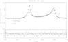 |
Fig. 1 Upper panel: pulse profiles measured by IBIS/ISGRI in the 20–40 keV energy band: crosses and diamonds represent the pulse profile before and during the Crab flare, respectively. Lower panel: significance in standard deviations of the difference between the pulse profile during and before the flare. |
2.2. Fermi
Fermi/LAT is a pair-conversion telescope that operates in the 30 MeV–300 GeV energy range with unprecedented sensitivity and resolution (Atwood & et al. 2009). In our analyses, we used all the events in the 0.1–300 GeV energy range belonging to the “diffuse” class, but rejected photons with zenith angles larger than 105° to avoid contamination from the Earth’s bright γ-ray albedo. We limited our sample to the data taken between 2010 September 1 to October 6. The analysis was performed using the ScienceTools, provided by the Fermi collaboration (Version v9r15p2). To obtain the source flux, we used the gtlike tool, which exploits a maximum likelihood method (Mattox et al. 1996). The instrument response function is P6_V3_DIFFUSE and the Galactic emission is reproduced using the model gll_iem_v02.fit2. All sources listed in the Fermi-LAT first year catalogue (The Fermi-LAT Collaboration 2010) within 7° of the Crab position and with a TS detection greater than 10 are taken into account in the likelihood analysis.
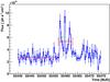 |
Fig. 2 Light curve of the Crab in the range 0.1–300 GeV with 12 h time bins. The green dashed line indicates the flux of the Crab estimated over all the Fermi operation period. The green solid line is the average flux between September 19 and 21, as reported by Buehler et al. (2010). The red lines represent the average flux before and during the flares (see Table 1). The time is expressed in Modified Julian Date. |
 |
Fig. 3 Exposure corrected Crab pulse profiles. Left panel: before the flares. Right panel: during the flares. The horizontal green and red lines indicate the off-pulse averages. |
Time intervals used to perform the Fermi analysis.
In Fig. 3, we compare the pulse profile measured
before and during the flares. We can estimate the contribution of the nebula, by assuming
that the pulsar emission is negligible in the phase ranges
φ < 0.25 and φ > 0.8. Before the flares,
the average rate of the nebular emission is  ,
whereas during the flare it is
,
whereas during the flare it is  .
After subtracting the contribution from the nebula, we compute the average rate of the
pulsed emission: before the flare it is
.
After subtracting the contribution from the nebula, we compute the average rate of the
pulsed emission: before the flare it is  ,
whilst during the flares it is
,
whilst during the flares it is  .
During the flares, we conclude that the flux from the nebula increased by a factor
3.33 ± 0.46. In contrast, the pulsar flux remained constant within the errors. This result
confirms the preliminary claim of Hays et al.
(2010).
.
During the flares, we conclude that the flux from the nebula increased by a factor
3.33 ± 0.46. In contrast, the pulsar flux remained constant within the errors. This result
confirms the preliminary claim of Hays et al.
(2010).
To study the high energy spectrum of the Crab, we exploit the maximum likelihood method for the dataset listed in Table 1. Following Abdo et al. (2010), we model the spectral emission from the Crab using two power-law components for the nebula, which represent respectively the synchrotron and IC emissions, and a power-law with an exponential cutoff to describe the pulsar contribution. As the flare is not pulsed, we fix the parameter related to the pulsar emission to these of Abdo et al. (2010), and assume that the IC contribution of the nebula has not changed during the flare. The only free parameters are the synchrotron contribution and the normalization of the Galactic emission. The synchrotron emission is found to increase from a flux of (5.6 ± 1.3) × 10-7 ph cm-2 s-1 to (32.4 ± 2.7) × 10-7 ph cm-2 s-1 in the 0.1–300 GeV band.
3. Discussion
To discriminate among the various models capable of reproducing the quasi-exponential
turnover of the synchrotron emission of the nebula that peaks below the LAT energy window,
we studied the Fermi data complemented by archival CGRO/COMPTEL data
(0.75–30 MeV). A single power-law cannot reproduce the pre-flare data
(χ2/d.o.f. ~ 44/15).
A power-law with a high energy exponential cutoff can instead reproduce the data
(χ2/d.o.f. ~ 4/14).
To model the nebular synchrotron spectrum, we used the following function
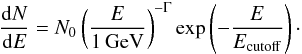 (1)The best-fit solution
yields Γ = −2.20 ± 0.08 and
N0 = (4.3 ± 1.9) × 10-10
ph cm-2 s-1 MeV-1. The difference between the
quiescent and flaring spectra can be understood by considering two different extreme cases
of either a constant power-law normalisation or a constant cutoff energy. In the former
case, an increase in the energy cutoff of a factor of nearly 5 (from 77 ± 15 MeV to
367 ± 45 MeV) is needed (as illustrated in Fig. 4).
This increase is averaged over the whole flaring period, thus represents a lower limit,
since in each single flare the cutoff energy might have been higher. In the latter case, the
spectral variability can be explained by raising the continuum normalization by a factor of
~5.
(1)The best-fit solution
yields Γ = −2.20 ± 0.08 and
N0 = (4.3 ± 1.9) × 10-10
ph cm-2 s-1 MeV-1. The difference between the
quiescent and flaring spectra can be understood by considering two different extreme cases
of either a constant power-law normalisation or a constant cutoff energy. In the former
case, an increase in the energy cutoff of a factor of nearly 5 (from 77 ± 15 MeV to
367 ± 45 MeV) is needed (as illustrated in Fig. 4).
This increase is averaged over the whole flaring period, thus represents a lower limit,
since in each single flare the cutoff energy might have been higher. In the latter case, the
spectral variability can be explained by raising the continuum normalization by a factor of
~5.
 |
Fig. 4 Crab spectral energy distribution in the 100 MeV–300 GeV energy range. The points with error bars are the Fermi detections before the flare (dark green), during the flare (red), and after the flare (light green). The black dashed line represents the contribution from the pulsar. The black dot-dot-dashed line represents the IC emission from the nebula. The blue and magenta dot-dashed and solid lines are the synchrotron nebula and the total emission before and during the flare, respectively. Arrows indicate the 95% confidence flux limits. |
We note that the non-detection of any significant hard X-ray variability during the flare does not allow us to differentiate between the two possibilities as several electron populations are probably present in the nebula. As reported by Aharonian & Atoyan (1998), the COMPTEL data are characterized by a flattening of the spectrum that can be ascribed to the synchrotron emission of a separate electron population confined in compact regions such as wisps or knots. The luminosity of this component is less than 1% of that of the whole nebula.
The cutoff in the synchrotron spectrum occurs at a characteristic frequency
νpeak ~ 4.2 × 10⁶ B γ2.
Provided that synchrotron radiation is the dominant mechanism through which particles
channel their energy, the maximum electron Lorentz factor obtained by equating
tsync to taccel is
γmax ∝ (B η) − 1/2,
where η ≥ 1 is the gyrofactor that characterizes the acceleration rate
 and
taccel = η E/qe B c.
This makes νpeak independent of B, leading to
an electron synchrotron energy cutoff ≈ 160η-1 MeV (see e.g.
Aharonian 2000). A higher value may imply that the
conditions in the accelerator differ from those in the emission region, e.g. there is a
lower magnetic field in the former, or that the synchrotron gamma-rays are produced in a
relativistically moving region, which produces a shift in the energy cutoff to higher
energies by the corresponding Doppler factor δ. In this scenario, a value
δ ~ 367/160 ≈ 2.3 would be required to explain the energy
cutoff obtained during the flaring episode.
and
taccel = η E/qe B c.
This makes νpeak independent of B, leading to
an electron synchrotron energy cutoff ≈ 160η-1 MeV (see e.g.
Aharonian 2000). A higher value may imply that the
conditions in the accelerator differ from those in the emission region, e.g. there is a
lower magnetic field in the former, or that the synchrotron gamma-rays are produced in a
relativistically moving region, which produces a shift in the energy cutoff to higher
energies by the corresponding Doppler factor δ. In this scenario, a value
δ ~ 367/160 ≈ 2.3 would be required to explain the energy
cutoff obtained during the flaring episode.
On the other hand, magnetic fields at the level of between ~300 μG and ~2 mG are found in the synchrotron nebula and wisps, respectively (see e.g. Hester 2008). Synchrotron radiation at ~1 GeV implies that γ ~ 3−10 × 109 in the emitting regions. Taking δ ~ 2.3, the comoving cooling timescale for those particles, taking an extreme value B ~ 2 mG, is ~0.3 d. The corresponding observer timescale would then be similar to the decay time of the peaks present in the Fermi lightcurve during the flaring period, ≲ 1 d. In contrast, the flares could be related to an enhanced electron population, and the spectral variability could be obtained by raising the continuum normalization by a factor of ~5 or by adding a hard very high energy electron population (leading to a photon index Γ < 1). In this case, a Doppler boosting may not be required, and the observed duration of the flares could correspond to the synchrotron timescale of PeV electrons embedded in magnetic fields ≲ 1 mG.
The duration of the three short flares limits the size of the emitting region(s) to
≲ 1015 cm. The peak luminosity of these flares is higher/brighter than
1035 erg/s, i.e.  0.5 ? of
the Crab spin-down luminosity, assuming an
isotropic distribution. The distance between the emitting region and the pulsar can thus be
constrained to be
0.5 ? of
the Crab spin-down luminosity, assuming an
isotropic distribution. The distance between the emitting region and the pulsar can thus be
constrained to be  6 × 10¹⁶
cm, i.e. not larger than 15% of
6 × 10¹⁶
cm, i.e. not larger than 15% of
the size of the bright synchrotron torus observed by Chandra and HST, and probably consistent with the half-width of this torus. The emitting region could therefore be linked to the interaction zone between the jet and the torus, which is found to have brightened in the HST image obtained on 2 October (Caraveo et al. 2010). The three flares separated by two days could possibly be related to various emitting knots in this region. Alternatively, gamma-rays could be produced within the jet itself. However, if the emitting region were moving at relativistic speeds, the emission would be radiated within an angle ~1/δ. For reasonable values of the jet inclination angle with respect to the line of sight (see e.g. Ng & Romani 2004), this scenario would make the flares difficult to detect.
To conclude, the flare relative short durations (<1 day), their soft spectrum, and the analysis of the pulse profile in the 0.1–300 GeV indicate that one or more compact portions (≲1015 cm or < 0.1′′) of the synchrotron nebula are responsible for the flares. In these region(s), freshly accelerated PeV electrons are rapidly cooling, causing the observed variability.
Acknowledgments
P.B. has been supported by the DLR grant 50 OG 1001.
References
- Abdo, A. A., Ackermann, M., Ajello, M., et al. 2010, ApJ, 708, 1254 [NASA ADS] [CrossRef] [Google Scholar]
- Aharonian, F. A. 2000, New Astron., 5, 377 [NASA ADS] [CrossRef] [Google Scholar]
- Aharonian, F. A., & Atoyan, A. M. 1998, in Neutron Stars and Pulsars: Thirty Years after the Discovery, ed. N. Shibazaki, 439 [Google Scholar]
- Atwood, W. B., Abdo, A. A., Ackermann, M., et al. 2009, ApJ, 697, 1071 [NASA ADS] [CrossRef] [Google Scholar]
- Buehler, R., D’Ammando, F., & Hays, E. 2010, The Astronomer’s Telegram, 2861 [Google Scholar]
- Caraveo, P., et al. 2010, The Astronomer’s Telegram, 2903 [Google Scholar]
- Courvoisier, T. J.-L., Walter, R., Beckmann, V., et al. 2003, A&A, 411, L53 [NASA ADS] [CrossRef] [EDP Sciences] [Google Scholar]
- Evangelista, Y., Campana, R., Capalbi, M., et al. 2010, The Astronomer’s Telegram, 2866 [Google Scholar]
- Ferrigno, C., Walter, R., Bozzo, E., & Bordas, P. 2010, The Astronomer’s Telegram, 2856 [Google Scholar]
- Hays, E., Buehler, R., D’Ammando, F., Grove, J. E., & Ray, P. S. 2010, The Astronomer’s Telegram, 2879 [Google Scholar]
- Heinke, C. O. 2010, The Astronomer’s Telegram, 2868 [Google Scholar]
- Hester, J. J. 2008, ARA&A, 46, 127 [Google Scholar]
- Jourdain, E., & Roques, J. P. 2009, ApJ, 704, 17 [NASA ADS] [CrossRef] [Google Scholar]
- Kanbach, G., Kruehler, T., Steiakaki, A., & Mignani, R. 2010, The Astronomer’s Telegram, 2867 [Google Scholar]
- Lebrun, F., Leray, J. P., Lavocat, P., et al. 2003, A&A, 411, L141 [NASA ADS] [CrossRef] [EDP Sciences] [Google Scholar]
- Lyne, A. G., Pritchard, R. S., & Graham-Smith, F. 1993, MNRAS, 265, 1003 [NASA ADS] [CrossRef] [Google Scholar]
- Markwardt, C. B. Barthelmy, S. D., & Baumgartner, W. H. 2010, The Astronomer’s Telegram, 2858 [Google Scholar]
- Mattox, J. R., Bertsch, D. L., Chiang, J., et al. 1996, ApJ, 461, 396 [NASA ADS] [CrossRef] [Google Scholar]
- Ng, C., & Romani, R. W. 2004, ApJ, 601, 479 [NASA ADS] [CrossRef] [Google Scholar]
- Segreto, A., & Ferrigno, C. 2007, in ESA SP, 622, 633 [Google Scholar]
- Shaposhnikov, N., Jahoda, K., Swank, J., et al. 2010, The Astronomer’s Telegram, 2872 [Google Scholar]
- Tavani, M., Striani, E., Bulgarelli, A., et al. 2010, The Astronomer’s Telegram, 2855 [Google Scholar]
- Tennant, A., Caraveo, P., Costa, E., et al. 2010, The Astronomer’s Telegram, 2882 [Google Scholar]
- The Fermi-LAT Collaboration, 2010, ApJ, 188, L405 [Google Scholar]
- Ubertini, P., Lebrun, F., Di Cocco, G., et al. 2003, A&A, 411, L131 [NASA ADS] [CrossRef] [EDP Sciences] [Google Scholar]
- Vedrenne, G., Roques, J.-P., Schönfelder, V., et al. 2003, A&A, 411, L63 [NASA ADS] [CrossRef] [EDP Sciences] [Google Scholar]
- Wilson-Hodge, C. A., Cherry, M. L., Baumgartner, W. H., et al. 2011, ApJ, 727, L40 [NASA ADS] [CrossRef] [Google Scholar]
All Tables
All Figures
|
Fig. 1 Upper panel: pulse profiles measured by IBIS/ISGRI in the 20–40 keV energy band: crosses and diamonds represent the pulse profile before and during the Crab flare, respectively. Lower panel: significance in standard deviations of the difference between the pulse profile during and before the flare. |
| In the text | |
|
Fig. 2 Light curve of the Crab in the range 0.1–300 GeV with 12 h time bins. The green dashed line indicates the flux of the Crab estimated over all the Fermi operation period. The green solid line is the average flux between September 19 and 21, as reported by Buehler et al. (2010). The red lines represent the average flux before and during the flares (see Table 1). The time is expressed in Modified Julian Date. |
| In the text | |
|
Fig. 3 Exposure corrected Crab pulse profiles. Left panel: before the flares. Right panel: during the flares. The horizontal green and red lines indicate the off-pulse averages. |
| In the text | |
|
Fig. 4 Crab spectral energy distribution in the 100 MeV–300 GeV energy range. The points with error bars are the Fermi detections before the flare (dark green), during the flare (red), and after the flare (light green). The black dashed line represents the contribution from the pulsar. The black dot-dot-dashed line represents the IC emission from the nebula. The blue and magenta dot-dashed and solid lines are the synchrotron nebula and the total emission before and during the flare, respectively. Arrows indicate the 95% confidence flux limits. |
| In the text | |
Current usage metrics show cumulative count of Article Views (full-text article views including HTML views, PDF and ePub downloads, according to the available data) and Abstracts Views on Vision4Press platform.
Data correspond to usage on the plateform after 2015. The current usage metrics is available 48-96 hours after online publication and is updated daily on week days.
Initial download of the metrics may take a while.