| Issue |
A&A
Volume 527, March 2011
|
|
|---|---|---|
| Article Number | A115 | |
| Number of page(s) | 16 | |
| Section | Astronomical instrumentation | |
| DOI | https://doi.org/10.1051/0004-6361/201015817 | |
| Published online | 04 February 2011 | |
Identifying XMM-Newton observations affected by solar wind charge exchange – Part II⋆
Department of Physics and AstronomyUniversity of Leicester, Leicester, LE1 7RH, UK
e-mail: jac48@star.le.ac.uk; sfs5@star.le.ac.uk; amr30@star.le.ac.uk
Received: 24 September 2010
Accepted: 21 December 2010
Aims. We wished to analyse a sample of observations from the XMM-Newton Science Archive to search for evidence of exospheric solar wind charge exchange (SWCX) emission.
Methods. We analysed 3012 observations up to and including revolution 1773. The method employed extends from that of the previously published paper by these authors on this topic. We detect temporal variability in the diffuse X-ray background within a narrow low-energy band and contrast this to a continuum. The low-energy band was chosen to represent the key indicators of charge exchange emission and the continuum was expected to be free of SWCX.
Results. Approximately 3.4% of observations studied are affected. We discuss our results with reference to the XMM-Newton mission. We further investigate remarkable cases by considering the state of the solar wind and the orientation of XMM-Newton at the time of these observations. We present a method to approximate the expected emission from observations, based on given solar wind parameters taken from an upstream solar wind monitor. We also compare the incidence of SWCX cases with solar activity.
Conclusions. We present a comprehensive study of the majority of the suitable and publically available XMM-Newton Science Archive to date, with respect to the occurrence of SWCX enhancements. We present our SWCX-affected subset of this dataset. The mean exospheric-SWCX flux observed within this SWCX-affected subset was 15.4 keV cm-2 s-1 sr-1 in the energy band 0.25 to 2.5 keV. Exospheric SWCX is preferentially detected when XMM-Newton observes through the subsolar region of the Earth’s magnetosheath. The model developed to estimate the expected emission returns fluxes within a factor of a few of the observed values in the majority of cases, with a mean value at 83%.
Key words: X-rays: diffuse background / solar-terrestrial relations / methods: data analysis
© ESO, 2011
1. Introduction
This paper follows that of Carter & Sembay (2008) (hereafter Paper I), whereby a set of approximately 180 XMM-Newton observations, taken between revolutions 52 and 1104 (March 2000 until December 2005), were analysed to search for cases of solar wind charge exchange emission (SWCX) occurring within the Earth’s magnetosheath or in near interplanetary space. In Paper I we searched for time-variable SWCX signatures and found that approximately 6.5% of the observations studied were affected. One case of SWCX showed an extremely rich emission line spectrum, which was attributed to a passing coronal mass ejection (CME) and has been discussed in detail by Carter et al. (2010). This paper extends the work of Paper I, to provide a complete sample, covering 3012 suitable XMM-Newton observations downloaded from the XMM-Newton Science Archive (XSA)1. We include data from between revolutions 28 and 1773 (February 2000 until August 2009).
SWCX processes occur at many locations within the solar system including planetary magnetosheaths, the corona of comets, within the heliosphere and at the heliospheric boundary where the outer reaches of the interplanetary magnetic field encounter that of the surrounding interstellar medium. Those charge exchange processes that result in the emission of X-rays occur for interactions involving a highly-charged solar wind ion, for example the bare oxygen ion O8+, and a donor neutral species, such as hydrogen in the case of geocoronal SWCX emission.
The possibilities for viewing exospheric SWCX emission in the vicinity of the Earth depend on the orbital and viewing constraints of the observatory in use, however one may be able to detect enhancements due to charge exchange occurring within the heliosphere. This will show fluctuations on longer timescales to SWCX occurring within the Earth’s exosphere (Cravens et al. 2001). SWCX emission from within the heliosheath (for example resulting from the helium-focusing cone) is a contributor to the X-ray emission from the supposed Local Hot Bubble in which the Sun resides (Koutroumpa et al. 2007, 2008), and to what level it contributes is under great debate. We concentrate, however, on SWCX emission occurring in the near vicinity of the Earth and use the time variable nature of this emission as our marker for selecting affected XMM-Newton observations.
In addition to the pioneering work noting the so-called Long Term Enhancements (subsequently known to be due to SWCX emission) within ROSAT observations (Snowden et al. 1995), the assignment of such enhancements to SWCX emission has also been observed in studies undertaken using data from Suzaku (Fujimoto et al. 2007; Bautz et al. 2009) and Chandra (Smith et al. 2005). Enhancements in soft X-ray band XMM-Newton spectra have been attributed to SWCX contamination in the literature (Snowden et al. 2004; Kuntz & Snowden 2008; Snowden et al. 2009; Henley & Shelton 2008). This has almost exclusively involved the comparison of multiple pointings of the same field which has enabled the serendipitous detection of the low-energy enhancement, most notably around the O vii helium-like triplet at approximately 0.56 keV. Observations of the Groth-Westfall Strip, Polaris Flare region and the Hubble deep field as discussed in Kuntz & Snowden (2008) were included in the analysis of Paper I as control cases for our method.
The XMM-Newton observatory (Jansen et al. 2001) has the largest collecting area in the band 0.2 to 10 keV of all X-ray telescopes currently in orbit and the European photon imaging camera (EPIC) suite of instruments on board (two MOS (Turner et al. 2001) and one pn (Strüder et al. 2001) CCD cameras) provide medium spectral resolution ( ). During various periods of its orbit and depending on observational constraints, XMM-Newton may view regions of the Earth’s magnetosheath which are predicted to exhibit the highest X-ray emissivity due to SWCX between highly charged solar wind ions and hydrogen in the Earth’s exosphere (Robertson et al. 2006, and references therein). We use data from the EPIC-MOS cameras to identify times of variability in a low energy band that is not mirrored in a higher energy band, to select those periods we suspect have been affected by variable SWCX.
SWCX emission can be considered as a contaminant by sections of the community wishing to study Galactic or Extragalactic sources beyond the heliosheath. Understanding the occurrence and nature of the emission is important therefore for the process of elimination from astronomical observations. However, SWCX emission can be used to provide diagnostics of the solar wind. X-rays emitted from the comas of comets have been suggested and used for this purpose (Cravens 1997; Dennerl et al. 1997; Lisse et al. 2001; Bodewits et al. 2007). A detailed study of the heavy ion constituents of a CME was discussed in Carter et al. (2010). In addition, exospheric-SWCX may be used to test models of dynamical processes within the Earth’s magnetosheath and the solar-terrestrial connection, such as flux-transfer events or boundary layer phenomena (Collier et al. 2010).
The layout of the paper is as follows. In Sect. 2 we describe the method employed to identify those observations of interest. In Sect. 3 we present the overall results for the whole sample studied and compare the occurrence of SWCX with the solar cycle. In Sect. 4 we describe fitting spectral models to cases of SWCX enhancement data. In Sect. 5 we discuss in more detail several of those observations affected by SWCX. In Sect. 6 we describe a model of the expected X-ray emission using the orbit of XMM-Newton and the solar wind conditions at the time of the observation. We finish with our discussion and conclusions in Sect. 7.
2. Data analysis
All observational data used in this study are available through the XSA where we extract the original data files (ODF). We consider observations taken by the EPIC-MOS (Turner et al. 2001) cameras (MOS1 and MOS2) using the full-frame mode only. Therefore the observations used provided an even sample across the mission and the event list data from the cameras could be combined if the same filter was used for both. We considered observations up to and including revolution 1773 (August 2009).
Individual observation event lists were created from the ODF for each EPIC-MOS camera and filtered for soft-proton contamination using the publicly available Extended Source Analysis Software (ESAS)2 package (mos-filter tool). At the time of data processing, ESAS was only available for the EPIC-MOS cameras. This tool fits a Gaussian to a histogram of in-field-of-view count rates in a high energy band (2.5 keV to 12.0 keV). Time periods with count rates beyond a threshold of ±1.5σ away from the peak of this Gaussian were removed by applying a good time interval (GTI) file to the event lists. The GTI files created for each EPIC-MOS event list were combined together to form one EPIC-MOS GTI file and this file was reapplied to both the MOS1 and MOS2 event lists to provide simultaneous coverage during each observation. Resolved point sources (from lists created for the 2XMM catalogue, Watson et al. 2009, using a minimum likelihood threshold ≥ 6), were removed from the field of view by extracting events in a circular region of 35 arcsec radius about the source position. Those observations judged, after a visual inspection (and prior to creation of any spectra, see Sect. 4), to show residual source contamination (the wings of the point spread function of the EPIC-MOS camera being evident in an image of the event file) passed through an additional spatial filtering stage using a larger extraction region to further clean the dataset. A more detailed description of the filtering steps and nature of soft proton contamination can be found in Paper I and Carter et al. (2010).
The method employed here followed the first steps as described in detail within Paper I. In summary, two lightcurves with bin size of 1 ks were created for each observation from events within the full field-of-view (radius of 13.3 arcmin). When both EPIC-MOS cameras were used during an observation and employed the same filter, events from both cameras were used to construct the lightcurves. The first lightcurve was chosen to represent the continuum, covering events with energies in the range 2.5 to 5.0 keV. The second lightcurve was extracted using events with energies in the range 0.5 to 0.7 keV to cover the strong SWCX emission from O vii and O viii (the line-band lightcurve). This energy range incorporates emission energies from the O vii triplet and resonance lines which are dominated by the forbidden line transition at 0.56 keV. Lightcurves were then exposure-corrected for periods removed during the filtering steps. As the MOS1 and MOS2 event files for each observation, prior to the lightcurve creation, were filtered using a single GTI file which is not energy specific, the exposure-coverage for each bin was the same for the line-band and continuum lightcurves. Therefore the same exposure-correction factor for an individual bin was applied to both lightcurves in this step. We keep bins of the lightcurve with at least 60% of the full exposure for that bin and reject the remaining bins (in contrast to Paper I when we kept all bins with at least 40% exposure). Lightcurves were rejected from further analysis if they were less than 5 ks in length. By increasing the strictness of the bin coverage thresholds, we reduced the incidence of type I errors (those incorrectly labelled detections), but ran the risk of increasing the number of cases that were incorrectly labelled as non-detections (i.e. not showing a deviance from the null hypothesis of a linear fit between the line-band and continuum (type II errors). We scaled each lightcurve by its mean to produce adjusted lightcurves. The count rates for the line-band and the continuum band were then always of the same order which facilitated the identification of periods of enhancement in the line-band lightcurve. An example of the combined-MOS lightcurve adjustment process can be found in Fig. 1 (panels top-left, top-right and bottom-left).
 |
Fig. 1 Lightcurve correction procedure example for observation with identifier 0150680101 (line-band (black), continuum (red) for panels top-left and bottom-left). Top left: example lightcurves showing a peak in the line-band that is not reflected in the continuum. Top right: exposure coverage for each bin, the threshold at 60% is marked by the red dashed line. Bottom left: lightcurves after the adjustments for exposure correction and scaling by the mean. Bottom right: example scatter plot for this observation. |
We plotted a scatter plot between the two bands (using the adjusted line-band as the dependent variable), shown in Fig. 1 (bottom-right). A linear model fit to each scatter plot was computed using the IDL procedure, linfit, which minimises the χ2 statistic.
We computed the reduced-χ2 for the fit, hereafter referred to as  , by dividing the χ2 by the number of bins minus one, to account for the reduction in the number of degrees of freedom made by fitting a linear model to the data. A high indicates that a significant fraction of the points deviate significantly from the best fit line. We expected these cases would be more likely to show variable SWCX-enhancement. In addition we computed the χ2 values for each individual lightcurve in terms of the deviation from the mean of that lightcurve. We calculated the ratio between the line-band and continuum χ2 values to add to our diagnostic (hereafter denoted as Rχ).
3012 observations made up the final sample to be used for further analysis. The results from Paper I showed us that those observations exhibiting both high and high Rχ were most likely to show near-Earth time-variable SWCX signatures. Observations that fulfilled these criteria were considered for further analysis, spectrally, temporally and with regard to the orientation of XMM-Newton.
3. Global results
All observations in our final sample, after any rejections as described below, were ranked by . The two highest ranked observations were observations of comets. Although resolved point sources have been removed, cometary X-rays are diffuse and will likely be spread over a large fraction, if not all of the field of view. We assume that the dominant variations in the line-band lightcurve that result in such high ranking are due to SWCX emission occurring within the cometary coma and not to any emission occurring within the vicinity of the Earth. We discuss the cometary cases in Sect. 3.3.
After ranking the observations, we were able to study those that exhibited the highest and Rχ in more detail on a case by case basis.
Observations were examined for residual point or extended sources that may contribute to the high variations in the line-band. Extended or diffuse residual sources that remain in the field of view will not affect this detection method providing no inherent variation occurs within these sources, as expected for sources outside the solar system, in either one of the bands. Cases were also examined for residual soft proton contamination. Although the files used in this analysis have been filtered for periods of soft proton flaring, residual contamination may remain. Excessive scatter due to residual soft proton contamination impedes the ability to identify periods of exospheric SWCX and will result in some type II errors in our sample. Also, if exospheric SWCX occurs throughout the entirety of the observation little or no variation can be seen in the line band, resulting in a rejection of this case. Excessive and simultaneous variations in both the line-band and continuum will result in a high yet a low value of Rχ. We concentrate our analysis therefore on cases that exhibit both high and high Rχ.
For some observations with short lightcurves, it was impossible to identify any time-periods of boosted line-band emission (the putative SWCX enhancement periods). These observations were disregarded as SWCX-enhancement cases. Also, the method described in this paper tested only for variable SWCX on short timescales. Spectral analysis of suspected SWCX cases was therefore only possible when a clear line-band enhancement period could be identified during the duration of the observation.
We find 103 observations in our sample that show indications of a time-variable exospheric SWCX enhancement, that are not excluded from consideration based on the reasons described above. All of these cases had a value greater than or equal to 1.2 and a Rχ value of greater than or equal to 1.0. These cases make up only ~20% of all observations that have values of and Rχ above these thresholds, indicating that although the values of and Rχ are indicators of a SWCX-enhancement, considerable inspection of an observation on a case-by-case basis is still required. The majority of cases in the whole sample have a Rχ value less than 1, indicating that there is more variation seen in the continuum compared to the line-band. The continuum incorporates the break energy at ~3.2 keV in the two-power law models of residual soft proton contamination (Kuntz & Snowden 2008). For higher intensity soft-proton flares, the slope of the power-law becomes flatter. Therefore the higher energy and wider continuum will have a greater variance than the softer, narrower line-band due to the presence of unfiltered residual soft protons.
The top 10 observations as ranked by are given in Table 1 (excluding those observations that had been rejected from consideration). Three of these top ten result from cometary observations, four were identified in the work presented in Paper I and three are new observations discovered during this analysis. Many of the highest ranked cases had previously been identified in the literature. It is our intention to make the full ranked list of observations used in this analysis publically available online in the future, most probably through the XMM-Newton EPIC background working group (BGWG) 3. We include a summary table listing the SWCX cases in Table A.1.
Highest ranked observation by .
A scatter plot of versus Rχ is given in Fig. 2. Those observations exhibiting both high and high Rχ but which do not show clear SWCX signatures (i.e. an enhancement in the mean-adjusted line-band lightcurve compared to that of the continuum) have been rejected from further analysis. We discuss the detection methods of SWCX cases in the literature, other than by a search for a time-variable low-energy component in Sect. 3.2. Cometary X-ray emission is discussed in Sect. 3.3.
 |
Fig. 2
|
In Fig. 3 we plot the total number of observations and the fraction of observations that show SWCX enhancements, versus the GSEX position of XMM-Newton at the mid-point of each observation. We can see from this figure that XMM-Newton is preferentially found on the subsolar side of the Earth when SWCX enhancements occur. In addition, the largest bin of the fractional plot occurs around the nominal magnetopause stand off distance, at approximately 10 RE. The XMM-Newton line-of-sight for these cases traversed the subsolar region (sunward side) of the magnetosheath, as expected according to the modelling work of Robertson et al. (2006). XMM-Newton viewing is constrained by the fixed solar panels and limits imposed to avoid directly observing the Sun, Moon and Earth and is only able to view the sunward side of the magnetosheath at certain times of the year (Carter & Sembay 2008).
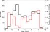 |
Fig. 3 Total number of observations (black) versus GSEX position and the fraction of observations detected with exospheric SWCX enhancements (red). |
We also consider the seasonal variation of the occurrence of SWCX in this sample. 64 SWCX cases occurred during the summer months (April until September inclusive) and 39 during the winter (October until March). More exospheric SWCX cases are expected in the summer months, as viewed by XMM-Newton (Carter & Sembay 2008).
3.1. Relationship with the solar cycle and solar wind
In Fig. 4 we plot the solar sunspot number4 from the latter half of Solar Cycle 23 and mark the times at which XMM-Newton observations with known SWCX (this paper, paper I and XMM-Newton exospheric-SWCX cases in the literature) occurred. We plot a histogram of the number of SWCX cases per half year, to remove any bias resulting from the seasonal constraints on pointing angle experienced by XMM-Newton. Each histogram bin starts at the start of summer (1st April) or start of winter (1st October). As expected for cases of exospheric SWCX, there are more cases at times of high solar activity around solar maximum than when approaching solar minimum. Also, for the cases from 2002 onwards and approaching solar minimum, we see a higher proportion of SWCX cases in the summer six-month period compared to the winter period, for the same year. The significance of this trend however should not be overstated due to the low number of cases in each bin.
 |
Fig. 4 Top panel: sunspot number versus time. Bottom panel: the coloured histogram of the fraction of observations affected by exospheric SWCX is binned into six month periods (blue – summer, black – winter). The total number of all observations for each period is noted above the bin. |
3.2. Multiple pointings of target fields
Multiple pointings towards the same target allow one to compare diffuse and extended emission spectral models that may exhibit spectral variations indicative of SWCX contamination. The long term enhancements of the ROSAT all-sky maps, which were subsequently attributed to SWCX, were first identified by comparisons between fields (Snowden et al. 1995). Kuntz & Snowden (2008) examined multiple XMM-Newton observations of the Hubble deep field, amongst other targets, and identified a proportion of their set affected to different degrees by SWCX emission. Bautz et al. (2009) inferred SWCX-enhancements in observations by Suzaku towards the cluster Abell 1795 after examination of a low-energy lightcurve revealed peaks coincident in time with enhancements in the solar wind proton flux as measured by Advanced Composition Explorer (ACE). Henley & Shelton (2010) used a large set of XMM-Newton observations to compare intensities from O vii and O viii lines from sets of observations with the same target pointings. They find no universal association between enhanced SWCX emission and the closeness of the the line-of-sight to the sub-solar region of the magnetosheath. In this paper we do see a tendency for XMM-Newton to be clustered around the sub-solar region for the SWCX cases, as discussed in Sect. 3.
One of the Henley & Shelton (2010) SWCX-enhanced cases is part of the data set used in this paper, however this was not detected by our method as no discernable variability occurred during the observation. Cases of SWCX occurring in the Earth’s exosphere, identified by detecting time-variable emission, have also been observed by Suzaku (Fujimoto et al. 2007; Ezoe et al. 2010). Carter et al. (2010) used a previous observation of a target field to constrain the diffuse X-ray emission inherent to that look direction to calculate the strength of SWCX emission lines associated with a CME passing in the vicinity of the Earth. The data set presented in the present paper contains a number of previously known cases of SWCX, however, not all of these were time variable and therefore were not picked up by the technique used here. They did however become tests of the ability of this method to identify SWCX-affected observations. One limitation of this technique is that SWCX emission occurring at an approximately steady state as part of any quiescent geocoronal X-ray emission will not be identified. In addition, any observed quiescent heliospheric SWCX will in general be several times stronger than any quiescent geocoronal X-ray emission, due to the increased integration lengths involved (Cravens et al. 2001). Although a combination of techniques would be ideal, this is not possible for the vast majority of single XMM-Newton pointings. The greatest advantage of this method is that observations are considered on an individual basis. An XMM-Newton user can make a judgement as to whether extra caution is required when analysing their results for possible SWCX-contamination.
3.3. Cometary emission
Comet Hyakutake was the first comet whose X-ray emission, as observed by ROSAT and RXTE (Lisse et al. 1996), was assigned to the SWCX emission process (Cravens 1997). This SWCX emission occurs from the interaction of the solar wind with neutral species that outgas from the comet as it enters the inner solar system, and the amount of out-gassing is dependent on the comet’s distance from the Sun. These neutral species are mainly water and its dissociation products. The SWCX emission must occur in cometary regions where photoionisation and destruction of the neutral species can occur. Water and hydroxyl ions have short lifetimes when exposed to solar UV photons and therefore survive the longest in the coma interior, whereas the dissociation products of water (along with CO providing the comet has a sufficiently high carbon abundance) can survive further into the outer coma regions. A detailed description of X-ray emission from comets, primarily using data from the Chandra observatory, can be found in Bodewits et al. (2007); Bodewits (2007).
Several XMM-Newton observations of comets were included in the sample in this paper. The and Rχ values for the comets are given in Table 2. The highest overall values of and Rχ occurred during observations of comets. Example line-band and continuum lightcurves from comet C2001 Q4 (Neat) (observation 0164960101) are shown in Fig. 5, where the line-band lightcurve clearly dominates and is highly variable. Also, an earlier observation of the same comet exhibited very different values of and Rχ. Although the upwind solar wind monitor ACE (level 2, combined instrument data, Stone et al. 1998) proton flux, also shown in this graph, is steady and not remarkable in intensity, the comet will more likely be sampling solar wind that originates from a different location in the solar corona. In Fig. 5 we have also plotted the O7+ to O6+ ratio, using data from the ACE SWICS instrument. This ratio varies slightly over the length of the observation but any fluctuations are not reflected in the XMM-Newton line-band lightcurve, further implying that the comet is sampling a different solar wind to that seen by ACE. The solar wind is a collisionless plasma and so its ion composition remains unchanged as it flows away from the Sun. Signatures of SWCX occurring throughout the solar system can therefore be used to infer the composition of the solar wind, which varies considerably throughout the solar cycle and with solar latitude. As cometary orbits are not restricted to the ecliptic plane they are ideal locations to study compositional signatures from solar wind originating from a variety of solar wind latitudes (Dennerl et al. 1997). Bodewits et al. (2007) was able to use cometary X-rays to distinguish emission resulting from three solar wind types: the cold and fast wind, the warm and slow wind and the warm and disturbed wind. A more complete discussion of cometary X-ray emission is beyond the scope of this paper.
XMM-Newton observation of comets within the data set.
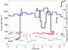 |
Fig. 5 Lightcurve from comet C2001 Q4 (Neat) that resulted in the highest |
3.4. Planetary emission
We include within the SWCX set an observation of the planet Saturn, taken on 1st October 2002. This observation has been comprehensively analysed by Branduardi-Raymont et al. (2010) who attribute the X-ray flux to emission from the planetary disk, produced by the scattering of solar X-rays and an additional fluorescent emission line of oxygen at ~0.53 keV originating from the rings. This observation was previously studied by Ness et al. (2004) but they did not investigate any low-energy variability. We find a high (2.9) and Rχ (2.3) in our time variability test and a distinct step in the line-band lightcurve, indicative of a SWCX enhancement, after the same filtering steps as to all other data sets have been applied, including source exclusion to remove emission from the planet and planetary exosphere. The initial source exclusion radius equates to ~3.7 RSaturn. Spectra from this observation were extracted from event files that had been additionally filtered with a larger extraction region of ~10.6 RSaturn. Even after this additional source extraction step the lightcurve production procedure yields metrics of and Rχ of 3.1 and 2.4 respectively. Two later observations of Saturn taken in 2005 were included within our sample but showed no evidence of SWCX enhancement. Therefore, we have no reason to reject this observation from the SWCX set. We were concerned that the planet’s movement through and possibly out of the field of view may have caused this effect. However, the dominant movement is in right ascension with a maximum speed of 8 arcsec per hour (Branduardi-Raymont et al. 2010), resulting in a shift of only 0.78 arcmin over the course of the 21 ks observation. In addition, resolved sources have been removed from the field of view as for all other observations.
4. Spectral analysis
We continue our study by observing the spectral signatures of new SWCX cases identified in this paper and in Paper I. We omit those SWCX observations that have been comprehensively investigated in the literature yet show no temporal variability in our tests. We also omit observations of comets. This set of observations which we have used for further study throughout this paper is hereafter known as the SWCX set and comprises 103 observations.
The Science Analysis System (SAS) software (version 9.0.0; http://xmm.esac.esa.int/external/xmm_data_analysis/) was used to produce spectral products and instrument response files for all observations of the SWCX set. The SAS accesses instrument calibration data in so-called current calibration files (CCFs) which are generally updated separately from SAS release versions. In this paper we used the latest public CCFs released as of February 2010.
For each exospheric-SWCX case we extracted spectra for the EPIC-MOS cameras for the suspected SWCX-affected period and for the suspected SWCX-free period. The SWCX-affected period was when the enhancement in the line-band lightcurve was judged (however not by a formal mathematical argument) to have occurred. The enhancement could have occurred at the beginning, middle or end of the observation. The remaining time periods in the observation made up the SWCX-free period. We used events from a circular extraction region, centred on detector coordinate positions (DETX, DETY = –50, –180), with an extraction radius of 16000 detector units or 13.3 arcmin. We also applied the flag and pattern selection expression ’#XMMEA_EM && PATTERN < = 12 && FLAG==0’. This pattern selection selects events within the whole valid X-ray pattern library for the EPIC-MOS and the flag selection removes events from or adjacent to noisy pixels and known bright columns. We produced instrumental spectral response files for each period. The instrument effective area files were calculated assuming the source flux is extended, filling the field of view and with no intrinsic spatial structure.
4.1. Spectral modelling
We knew from the work of Carter et al. (2010) that exospheric SWCX can occur throughout the entirety of an observation, although the line-band lightcurve may show an enhanced and a steady-state period. We used the spectra from the apparent SWCX-affected period as the source spectra and that from the apparent SWCX-free period as the background to produce a difference spectrum. The difference spectrum therefore provides a lower limit to the SWCX enhancement that has occurred during an observation. Providing the particle-induced background is reasonably constant over the duration of the observation (at most ± 10%, De Luca & Molendi 2004) this factor will be eliminated. An inspection of the difference spectra was made for energies above 2.5 keV, to check for the presence of significant variable residual soft-proton contamination. Each SWCX-case showed a count rate statistically consistent with zero above this energy.
We modelled the resulting difference spectrum for each SWCX case with a standard model of emission lines. The spectrum from MOS1 and MOS2 were fitted simultaneously, although a global normalisation parameter for the MOS2 spectrum was allowed to vary. The relative line strengths for a particular ion species below 1 keV, for example O vii (which involves seven separate transitions including the O vii triplet), were set using the velocity dependent cross-sections of laboratory charge exchange collisions between highly charged ion and atomic hydrogen, as found in Bodewits (2007). We assumed a solar wind speed of 400 km s-1 for these cross-sections. We also added emission lines from Ne x at 1.022 keV, Mg xi at 1.330 keV and Si xiv at 2 keV. There may be emission from other ion species present in the spectra, such as from highly charged iron or aluminium (as seen in Carter et al. 2010), but we wished to simplify the model applied to a general case and the dominant SWCX emission lines are found below 1 keV. We fixed the relative normalisations of the minor transitions to that of the principal transition for each ion species. The principal, dominant transition in the case of C v, N vi and O vii is the forbidden line transition. The principal ion transitions used in this modelling can be seen in Table 3.
Principle ion species emission lines used in the model, plus any minor emission line energies used (see text).
We used Version 12.5.0 of the XSPEC5 X-ray spectral fitting package to perform this analysis. We fitted the model to each difference spectrum by minimising the χ2 statistic. We calculated the modelled flux and 1-sigma errors on the flux between 0.25 and 2.5 keV for each EPIC-MOS instruments. The keyword giving the area collected in the spectral extraction (BACKSCAL) was converted into units of steradians and used to convert the individual flux values to units of keV cm-2 s-1 sr-1. Fluxes presented here onwards are for a combined error weighted-average EPIC-MOS flux. The error on the flux was calculated from the individual flux errors, combined in quadrature. A histogram of the total spectrally fitted flux for each of the SWCX set can be seen in Fig. 6. The minimum flux we observed for a SWCX case was 2.2 keV cm-2 s-1 sr-1 (observation id. 0112490301) and the maximum 50.1 keV cm-2 s-1 sr-1 (observation id. 0085150301, Carter et al. 2010).
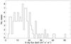 |
Fig. 6 Histogram of total spectrally fitted flux between 0.25 and 2.5 keV for the SWCX set. |
The relative strengths of the component lines to the SWCX spectral model varied considerably within the SWCX set. Individual line fluxes were calculated by finding the best fit model using all lines, as described above, then setting other line normalisations to zero in XSPEC. The flux for the individual ion species contribution was calculated in the range 0.25 to 2.5 keV.
High O7+ to O6+ and magnesium to oxygen ratios are used as indicators of the presence of CME plasma (Zhao et al. 2009; Richardson & Cane 2004; Zurbuchen & Richardson 2006). O vii is the dominant SWCX ion-species in the majority of cases. In Fig. 7 we plot the ratio of the fluxes of the lines Mg xi/O vii to O viii/O vii (using those oxygen transitions available to us within our X-ray spectral band). To look for plasma signatures with the highest charge states we only plot those cases where the normalisation of the numerator in the ratio is well constrained. Three observations are constrained to have both a ratio of Mg xi/O vii > 0.6 and O viii/O vii > 1.0. One of these (with identifier 0085150301) was the observation previously assigned to a passing CME and described in Carter et al. (2010). These observations are therefore possible candidates for having observed CME plasma with XMM-Newton and are listed in Table 4. We quote the lower limit to the ratio in the case where the O vii flux is badly constrained, i.e. very weak. In this table we also quote the mean value of the O7+ to O6+ ratio during the period of the observation, using values taken from the ACE SWICS instrument. This data was only available in two of the cases in the table. As ACE is found at Lagrangian point L1, we have time shifted the solar wind data to account for the travel time to Earth, based on the mean speed of the solar protons during the XMM-Newton observation. Expected O7+/O6+ ratios for the slow and fast solar wind are 0.27 and 0.03 respectively (Schwadron & Cravens 2000). Both of the observations with ACE SWICS data surpass both the nominal slow and fast values by a considerable margin and would suggest that ACE detected a CME plasma. Although the identification of CME plasma generally involves many more criteria to be satisfied, XMM-Newton could provide supplementary spectral evidence to studies employing in-situ dedicated solar wind monitors in the field of solar system space science.
 |
Fig. 7 Ratio of Mg xi/O vii to O viii/O vii where available for the SWCX set. Where appropriate we mark the lower limit (red). |
To test if any relationship exists between the flux of the SWCX lines and increased solar wind flux, we plot in Fig. 8 the observed flux versus the difference in the mean solar wind proton flux (as measured by ACE) between the SWCX-affected and SWCX-free periods. We have again time-shifted the ACE data to account for the distance between L1 and the Earth. Although there is considerable scatter amongst these values, there is a positive correlation between line flux and solar wind proton flux. We include in the plot the linear fit as found by the IDL procedure linfit. Proton flux, for our SWCX set, is a good indicator of the presence of SWCX-enhancement, if not the level of this enhancement. This is in contrast with the results of Henley & Shelton (2010), whose SWCX cases were considered to be due to SWCX occurring within the heliosphere and therefore no correlation would be expected between an upstream solar wind monitor and any SWCX enhancement. Heliospheric SWCX is expected to vary on longer timescales than exospheric SWCX and therefore will be harder to identify by the technique in this paper. However, at certain times of the year XMM-Newton may have a line-of-sight that passes through the helium focusing cone, that could potentially produce a variable signal in the line-band that may be detectable by this technique (variations over a few hours, Koutroumpa et al. 2007). We discuss this possibility further in Sect. 6.1. The flux variations seen within our SWCX set are therefore due to local X-ray emission in the vicinity of the Earth.
SWCX set observations exhibiting the highest Mg xi/O vii and O viii/O vii ratios, or the lower limit (95% confidence) to this ratio when O vii is badly constrained.
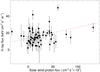 |
Fig. 8 Observed flux versus mean solar wind proton flux. The red dotted line indicates a linear fit to the data. |
5. Example cases of SWCX enhancement
In this section we comment on the three newly identified exospheric cases from Table 1. Lightcurves for each, over-plotted with the solar proton flux as recorded by ACE, are given in Fig. 9. The solar proton lightcurves have been adjusted for the distance between ACE and the Earth by adding a delay based on the distance to ACE and the mean solar proton speed, assuming a planar wavefront travelling on the Sun-Earth axis. We also plot a difference spectrum for each observation by combining data from both EPIC-MOS cameras and over-plot the best fit model to the data, as described in Sect. 4. Individual fluxes for a selection of prominent lines are given for each case in Table 5.
-
observation 0150610101 (revolution 0623). The line-bandlightcurve shows a period of enhanced count rate at the beginningof the observation. The ACE solar proton flux israised at the beginning of the lightcurve and reduces as thelightcurve progresses. The difference spectrum exhibitsemission at O vii, O viii, alongwith evidence of carbon emission below0.5 keV. The flux observed between 0.25 and2.5 keV was 20.6 keV cm-2 s-1 sr-1;
-
observation 0054540501 (revolution 0339). The line-band lightcurve shows an enhancement during the latter part of the observation, which is also observed in the ACE solar proton flux. The difference spectrum exhibits emission in the oxygen band, along with evidence of carbon emission below 0.5 keV. The flux observed between 0.25 and 2.5 keV was 7.9 keV cm-2 s-1 sr-1;
-
observation 0113050401 (revolution 0422). The line-band lightcurve shows a period of enhanced count rate at the beginning of the observation. A short enhancement period is seen in the ACE solar proton flux and the overall magnitude of this flux is much higher than the other two cases in this section. The flux observed between 0.25 and 2.5 keV was 25.9 keV cm-2 s-1 sr-1.
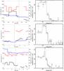 |
Fig. 9 Example cases of SWCX enhancement, for (top row) observation id. 0150610101, (middle row) observation id. 0054540501 and (bottom row) observation id. 0113050401. Each left-hand panel shows the line-band (black) and continuum band (red) non-mean-adjusted lightcurves along with the solar proton flux (blue, right-hand y-axis). The split between the SWCX-free and SWCX-affected period is indicated by the dashed vertical line. In the right-hand panels we show the combined EPIC-MOS difference spectrum and the model fitted to the data for each case (solid line). |
Most prominent ion line fluxes for example cases.
6. Modelling the expected emissivity
The expected X-ray emissivity of SWCX emission from the solar wind interaction with the magnetosheath can be estimated from the integrated emission along the line-of-sight for the observer. We have developed a model, applicable to local interplanetary space, to calculate this emission. We have not attempted to include any contribution from further into the heliosphere, as to increase the integration length would lead to greater uncertainty in the underlying parameters of the solar wind on large spatial scales. We assume that the solar wind parameters used in the model are approximately constant (excluding the magnetosheath region) along the line-of-sight. The emissivity expected (Cravens 2000) is given by the expression:  (1)where α is the efficiency factor dependent on various aspects of the charge exchange such as the interaction cross-section and the abundances of the solar wind ions,
  is the density of the solar wind protons,
  is the density of the neutral species and ⟨ g ⟩ is their relative velocity.
For each observation under study in Paper II, we wish to test whether any relationship exists between the total SWCX flux seen and the theoretical integrated X-ray emission along the line-of-sight (based on Eq. (2), Cravens 2000).  (2)
(2)
We take data describing the conditions in the solar wind from ACE (Level 2 processed data, merged instrument data using hourly averages) at the time of each observation. We needed to apply a delay to the signal received, to account for the separation between ACE and the Earth. This delay will be time variable and will depend on the speed and orientation of the solar wind. However, as a first approximation, we have taken the average solar proton speed of the data and assumed a planar wavefront travelling anti-sunward perpendicular to the GSEX axis. We calculate the delay required for the wavefront to travel from ACE to the Earth.
Throughout this work we assume a geocentric solar-ecliptic coordinate system (GSE), where positive X is directed from the Earth to the Sun, positive Y opposes planetary motion and positive Z is parallel to the direction towards the north ecliptic pole.
Then for each time bin of an observation:
-
we extract the solar wind proton velocity and temperature fromthe ACE data, and for these parameters wecalculate a thermal velocity and average speed, usingEqs. (3) and (4);

-
we estimate the position of the magnetopause, based on the model of Shue et al. (1998). To do this we use information regarding the strength and direction of the interplanetary magnetic field (Bz component). We currently assume that the magnetopause shape is symmetrical about the GSEX axis and place the magnetopause standoff distance along this axis.
-
using the magnetopause location as a guide, we approximate the position of the bow shock. We base the shape on a simple parabola and calculate the bow shock standoff distance using the solar wind pressure and the relationship in Khan & Cowley (1999). The magnetopause and bowshock together define the magnetosheath region;
-
we create an Earth-centric square image for use in subsequent steps. The side length of the image is 200 RE. This image is divided into cells, with side length 0.5 RE. The magnetosheath shape is projected onto this image. We are able to use an image rather than a cube due to the assumption made previously regarding the symmetry of the magnetosheath shape about the GSEX axis;
-
we find the neutral density of hydrogen atoms for each cell. We use the Østgaard et al. (2003) model for neutral hydrogen density profiles around the Earth, but limit this to a minimum density of 0.4 cm-3 (Fahr 1971).
-
we determine the line-of-sight of the XMM-Newton pointing through the grid by extracting the relevant information from the ODF and converting the positions and target pointing direction to the GSE coordinate system;
-
we find the velocity and density of the solar wind for each cell, (Spreiter et al. 1966; Kuntz, priv. comm.). As the solar wind passes the bowshock and enters the magnetopause its density increases (by about a factor of four in the subsolar region, as compared to the unperturbed value), and the velocity drops to about one tenth;
-
the value of α is dependent on the abundances of the ion species contributing to the charge exchange process, along with the cross-section and energy of each interaction with the neutral donor in the energy band of interest. The neutral donor is hydrogen in the geocoronal case. The relative abundances found in the solar wind vary considerably with solar wind state. The composition of the solar wind generally follows abundances seen in the photosphere, but can vary by up to a factor of about 2 (fast wind) or 4 (slow wind) for elements with first ionisation potential (FIP) below the Lyman-α limit of 10.2 eV (Richardson & Cane 2004, and references therein). However, we use the slow solar wind abundances for an ion species with respect to oxygen, as listed in Schwadron & Cravens (2000). We use an oxygen to hydrogen ratio of 1/1780 for solar wind speeds of ≤ 650 km s-1 or 1/1550 for speeds above this threshold. For this modelling we consider contributions to the emission from the principal and minor transitions as described in Sect. 4.1. Cross-sections for charge exchange transitions are dependent on solar wind speed. We calculate an α map with the same dimensions and binning as that of the Earth grid and populate this map with values of α depending on the speed of the solar wind, unperturbed outside of the magnetosheath or perturbed inside the magnetosheath as described above;
-
we multiply the solar wind velocity, solar wind density and neutral hydrogen density together for each of the cells in the line-of-sight and multiply this value by the efficiency factor α for each cell. This is the emissivity of each cell.
-
we sum all cells in the line-of-sight, accounting for the number of cells included in the integral, to give the value of the emissivity metric, approximating Eq. (2).
There are some known limitations to this model, such as:
-
there are no magnetosheath cusps (increased density ormodifications to the velocity of the solar wind specific to theseregions) included in the Spreiter approximation;
-
the neutral hydrogen has been modelled as spherically symmetrical about the Earth. However, there may be density enhancements in regions of the exosphere;
-
the abundances of the solar wind are not constant, but will change for example with the phase of the solar cycle or the injection of plasma from a CME;
-
the magnetopause and bow shock standoff distances have been assumed to be on the GSEX axis, this may not be the case;
-
the interstellar neutral density may be significantly different from that of the approximate limiting density applied in this model.
We also consider an adapted model, whereby the α calculated is dependent on the relative abundances of O6+ and O7+. We use the ratio of these ionisation states, taken from the ACE merged, hourly-averaged data sets to re-calculate the abundance of O7+ assuming the initial O6+ and O7+ abundances as found in Schwadron & Cravens (2000). We then re-calculate the value α and the subsequent line-of-sight flux. These results will be referred to as the Model-2 results and will be discussed in Sect. 6.1.
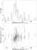 |
Fig. 10 Top: histogram of the modelled fluxes. Bottom: observed flux (0.25 to 2.5 keV) versus the modelled flux for the SWCX set. A line (dashed, red) of gradient unity has been added to the graph to aid the eye. |
6.1. Modelled emission results
Modelled lightcurves were produced for each SWCX case when there were data available from ACE. We split the modelled emission based on the time periods used for the creation of the spectra in Sect. 4.1. The resultant flux is the difference between the mean modelled flux during the SWCX-affected and the SWCX-free periods. A histogram of the modelled fluxes is given in Fig. 10 (top panel), along with a scatter plot showing the observed flux versus the modelled resultant flux for each exospheric-SWCX case (bottom panel). In general there is a positive correlation between the modelled and observed flux. For a few cases the modelled flux is negative. This happens when the SWCX-affected period, as determined using an enhancement seen in the observed line-band lightcurve, occurred in the opposite period to the maximum expected modelled flux. The enhancement in the observed line-band lightcurve occurred sufficiently far away in time from any peak seen in the modelled X-ray flux lightcurve.
In Fig. 11 (top-row) we show modelled lightcurves for the three top new cases of Table 1. Contributions from the model were only taken for the periods where there were counts in the XMM-Newton lightcurves (periods not removed during the filtering process). Example lightcurves of cases where the modelled flux is negative are given in the first two panels of the second row of Fig. 11. We also plot a modelled lightcurve when SWCX was not detected (below the thresholds for and Rχ) in the bottom-right panel of the same figure. In this case the line-band lightcurve does not vary significantly. The modelled emission in this case is small compared to the SWCX cases presented in the other examples.
 |
Fig. 11 Example modelled (blue, in keV cm-2 s-1 sr-1, left-hand y-axis) and XMM-Newton line-band (black, ct s-1, right-hand y-axis) lightcurves. Observations with identifiers (top-left) 0150610101, (top-middle) 0054540501, (top-right) 0113050401 show the model lightcurve generally following the shape of the XMM-Newton lightcurve. Observations (bottom-left) 0141150101 and (bottom-middle) 0150320201 show the modelled lightcurve peak in a different period to the XMM-Newton lightcurve and (bottom-right) 0301410601 is an example from an observation without a SWCX enhancement. Five panels show the split between the SWCX-affected and SWCX-free periods (vertical dashed line). |
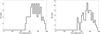 |
Fig. 12 Histograms of the first eigenvalues percentage contribution to the total, for the modelled emission versus the XMM-Newton line-band lightcurve (left) and versus solar wind flux (right). |
We wished to test how well the individual modelled flux lightcurve tracked that of the line-band lightcurve for each observation. We also wanted to determine the most dominant parameter in the modelling of the expected emission. To do this we applied principal component analysis to the model versus the line-band lightcurve and the model versus the solar wind flux. We calculate the correlation matrix between a linear fit to the relationship between each pair of values, for each exospheric-SWCX case. We calculate the correlation rather than the covariance matrix as the scale ranges of the data differ by a large amount and so by using the correlation coefficients we standardise the data. We use the primary eigenvalue of this matrix to calculate the percentage contribution along the assumed linear relationship between these lightcurves. Histograms of these percentage contributions can be seen in Fig. 12. The histogram (left) shows that the X-ray lightcurve is generally correlated with the modelled lightcurve, as the first principal component percentages are high (with a mean of 73.7%). The histogram (right) also shows high first principal component percentages (with a mean of 73.6%), which suggests that in the vast majority of cases the model is dominated by the incoming solar wind flux. The lowest eigenvalue when comparing the modelled emission to the line-band lightcurve occurred for the observation with the identification number 0101440401. Modelled and line-band lightcurves for this case are shown in Fig. 13. We also plot the component lightcurves that make up the total modelled lightcurve from within the magnetosheath and from beyond the bow shock. The contributions from the magnetosheath region in this case dominates the modelled lightcurve. XMM-Newton is found anti-sunward of Earth during this observation and so the line-of-sight of XMM-Newton passed through the flanks of the magnetosheath. This region is less well defined in our model due to the approximations of the shape of the bowshock boundary and the extrapolation of the values used to perturb both the solar wind density and velocity in this region. The overall modelled emission was very low for this case, compared with the top-row cases of Fig. 11.
In Fig. 14 (top) we plot the modelled resultant flux versus the average length of the line-of-sight through the magnetosheath (between the magnetopause and the bow shock). In Fig. 14 (bottom) we present the observed flux versus the average length of the line-of-sight through the magnetosheath. There is no discernible general relationship between the modelled or the observed flux with the length of line-of-sight through the magnetosheath.
We investigate when the model and observed fluxes are discrepant by calculating the fractional difference between the observed and modelled fluxes ((observed-modelled)/observed flux). In Fig. 15 (top panel) we plot this fractional difference versus the maximum solar wind flux during each observation, along with a histogram of the fractional difference values. The mean of these fractional differences was +0.17 and the modal bin of the histogram was for values between 0 and 1. A large proportion (approximately 60%) of the modelled cases had a fractional difference between –1 and 1. The most discrepant cases occurred when the solar wind flux was low (compared to the maximum solar wind flux of these exospheric-SWCX cases). The solar wind plasma flow around the Earth’s magnetosheath in these cases has been badly described by the model.
The observation with the largest absolute fractional difference had identifier 0041750101. This case was similar to cases (bottom-left and bottom-right) of Fig. 11 when the modelled lightcurve peaked in the alternative (SWCX-free) period to the enhancement in the observed line-band lightcurve (SWCX-affected).
We also wished to consider whether the fractional difference was due to some underlying emission with temporal variability occurring in near-heliospheric space, in particular to that of the helium focusing cone (Weller & Meier 1974). We consider cases within the SWCX set that occur within 10° of the cone’s direction (73.9° ecliptic longitude and − 5.6° ecliptic latitude, Witte et al. 1996). As the integration length for the model is relatively short compared to the spatial extent of the helium focusing cone and size of Earth’s orbit, only those observations taken when XMM-Newton is within this region are of importance. We find 4 cases within this region. These cases are marked in red in Fig. 15. A statistical analysis, repeatedly drawing 4 random cases from the SWCX set, indicates that we obtain an average fractional difference for the 4 random cases to be greater than that of the 4 helium focusing cone cases 28% of the time. We therefore have no evidence to suggest that temporal variability originating in the helium focusing cone is a significant component of the observed-to-modelled flux discrepancy.
 |
Fig. 13 Example modelled lightcurve (blue, left-hand y-axis) with the XMM-Newton line-band (black, right-hand y-axis), for the case where the first eigenvalue percentage contribution was the lowest when comparing the modelled flux and XMM-Newton lightcurves. The contribution to the modelled lightcurve from the magnetosheath (green-dashed) and region past the bow shock (plum-dashed) are also shown. The SWCX-affected period was taken between the vertical dashed lines. |
 |
Fig. 14 Line of sight length through the magnetosheath versus the modelled flux for the SWCX set (top) and the observed flux for the SWCX set (bottom). A mean error on the observed flux bar is given to the right of the bottom plot. |
 |
Fig. 15 Fractional difference between (top) the observed and modelled flux and (bottom) the observed and Model-2 flux, versus the maximum solar wind flux. Also included in each panel is a histogram of the fractional differences. Cases where XMM-Newton is found within the helium focusing cone are marked in red. |
We also compute the fractional differences between the observed and modelled flux values for the Model-2 results. These are shown in Fig. 15 (bottom panel). The peak of the distribution lies in the same bin as that of Fig. 15 (top panel), although there is a greater variance seen in the differences. We conclude that for the SWCX set cases, no benefit has arisen by using a compositionally-variable dependent model as opposed to the simple model. We continue our discussion based on the simple model results only.
We split the fractional difference values into two sets; for cases where this value is <–1.5 or >1.5 (bad), or any other value (good). In Fig. 16 we plot histograms of the mid-observation position of XMM-Newton (in GSE coordinates, GSEX, Y and Z) for each observation for the good and bad sets. We performed a Kolmogorov-Smirnov test on the three pairs of good and bad sets. The probabilities that the good and bad sets are drawn from the same sample distribution were 0.22, 0.002 and 0.79 for GSEX, GSEY and GSEZ respectively, indicating that for the GSEY coordinates, the good and bad sets are statistically different. The good set for the GSEY positions are skewed towards negative values and there are relatively more observations in the bad set in the positive direction. We repeat the test using mid-observation position of XMM-Newton expressed in Geocentric Solar Magnetospheric (GSM) coordinates. These differ from the GSE coordinates as the GSMY axis is perpendicular to the Earth’s magnetic dipole (the Xaxis is unchanged). The Kolmogorov-Smirnov test results were 0.22, 0.004 and 0.28 for the GSMX, GSMY and GSMZ respectively. The Ycoordinate result remains significant. Therefore we postulate that the model is better at describing the conditions seen by XMM-Newton when the Ycoordinate is negative.
The simplifications used in this model to describe the flanks of the magnetosheath in terms of shape, solar wind density and velocity may mean that the model is less robust in this region. We assumed cylindrical symmetry about the GSEX axis, however, the magnetosheath will be non-symmetrical in shape, suffering for example magnetosheath erosion along one side of the magnetopause (along the dusk side, or GSEY, Owen et al. 2008), a full discussion of which is beyond the scope of this paper. The incoming solar wind is expected from the GSEY positive direction, determined by the flow of the solar wind along the Parker Spiral as it emanates from the Sun. It is in this region that we expect the greatest differences in shape from the simplified magnetosheath we have used in our modelling steps and it is here that we see the largest absolute fractional differences between the observed and modelled fluxes. It is clear that although the model can estimate the observed flux within a factor of ~2 in approximately 50% cases, there are still many occurrences when the local physical conditions combine so that the simple model does not explain the observed flux adequately.
 |
Fig. 16 Histograms of mid-observation (left) GSE-X, (middle) GSE-Y and (right) GSE-Z XMM-Newton positions for good (blue) and bad (red) fractional differences between the observed and modelled fluxes. The histogram bins have been offset from one another in the plot, for ease of viewing. |
7. Discussions and conclusions
We have identified 103 XMM-Newton observations, 3.4% of the sample studied, when temporally variable SWCX emission was present in the data. The method of this paper has been able to identify cases of temporally variable SWCX from within a large sample of XMM-Newton observations. These cases were taken from those observations presenting the highest and Rχ values. The corresponding occurrence rate within the sample used in Paper I was ~6.5%. The data for this paper covered a wider range in time compared to Paper I. The level of detection can be attributed to the reduction in solar activity as this time range extended into a period towards solar minimum. There will be many more XMM-Newton observations affected by SWCX, either occurring within the exosphere or near-interplanetary space, such as within the helium focusing cone, or at the heliospheric boundary and undetectable here. SWCX occurring within the heliosheath will generally vary over longer periods than exospheric SWCX and so is more suited to detection by observation-to-observation comparison (e.g. observations within the studies of Kuntz & Snowden 2008; Henley & Shelton 2010). Enhancements from the helium focusing cone will produce some temporal variation but are strongly constrained by viewing geometry. The method presented in this paper is only able to identify time-variable SWCX which varies over the length of an observation and therefore the level of contamination quoted in this paper can only provide a lower limit to the occurrence of exospheric SWCX as observed by XMM-Newton. When SWCX emission is only slowly varying or constant over an exposure it will be undetectable by this method. There will also be cases which have slipped detection due to a high percentage of the observation data being removed by the flare-filtering process, resulting in short lightcurves that are excluded from our analysis. As increased concentrations of solar wind ions in the magnetosheath are expected to mirror increases in the general flux of the solar wind, increased levels of SWCX emission are expected precisely when the flux of solar proton increases. If the on-board radiation monitors of XMM-Newton detect a dangerous environment for the satellite, the science instruments are switched into a safe mode which invariably leads to the loss of high SWCX emission periods being available for detection within our sample. Even after soft-proton flare-filtering has been applied to the data, considerable proton-contamination may be present. This can result in a significant scatter when plotting either the line-band or continuum lightcurve, whilst potentially masking a clear enhanced period of SWCX-emission during the observation. The level of residual soft-proton contamination may mean that the observation is completely rejected by an observer. If the user does indeed proceed to process the data, the limits presented here on and Rχ may be useful to guide any further analysis as to whether extra caution should be taken to account for potentially high levels of time-variable SWCX contamination.
Acknowledgments
We thank Anthony Williams for helpful discussions regarding constituents of the solar wind. We thank the anonymous referee for their suggestions that have greatly enhanced this paper. The authors gratefully acknowledge funding by the Science and Technology Facilities Council, UK.
References
- Bautz, M. W., Miller, E. D., Sanders, J. S., et al. 2009, PASJ, 61, 1117 [NASA ADS] [Google Scholar]
- Bodewits, D. 2007, Ph.D. Thesis, University of Groningen [Google Scholar]
- Bodewits, D., Christian, D. J., Torney, M., et al. 2007, A&A, 469, 1183 [NASA ADS] [CrossRef] [EDP Sciences] [Google Scholar]
- Branduardi-Raymont, G., Bhardwaj, A., Elsner, R. F., & Rodriguez, P. 2010, A&A, 510, A73 [NASA ADS] [CrossRef] [EDP Sciences] [Google Scholar]
- Carter, J. A., & Sembay, S. 2008, A&A, 489, 837 [NASA ADS] [CrossRef] [EDP Sciences] [Google Scholar]
- Carter, J. A., Sembay, S., & Read, A. M. 2010, MNRAS, 402, 867 [NASA ADS] [CrossRef] [Google Scholar]
- Collier, M. R., Sibeck, D. G., Cravens, T. E., Robertson, I. P., & Omidi, N. 2010, Eos Trans. AGU, 91, 213 [NASA ADS] [CrossRef] [Google Scholar]
- Cravens, T. E. 1997, Geophys. Res. Lett., 24, 105 [NASA ADS] [CrossRef] [Google Scholar]
- Cravens, T. E. 2000, ApJ, 532, L153 [NASA ADS] [CrossRef] [PubMed] [Google Scholar]
- Cravens, T. E., Robertson, I. P., & Snowden, S. L. 2001, J. Geophys. Res., 106, 24883 [Google Scholar]
- De Luca, A., & Molendi, S. 2004, A&A, 419, 837 [NASA ADS] [CrossRef] [EDP Sciences] [Google Scholar]
- Dennerl, K., Englhauser, J., & Trümper, J. 1997, Science, 277, 1625 [NASA ADS] [CrossRef] [Google Scholar]
- Ezoe, Y., Ebisawa, K., Yamasaki, N. Y., et al. 2010, PASJ, 62, 981 [NASA ADS] [Google Scholar]
- Fahr, H. J. 1971, A&A, 14, 263 [NASA ADS] [Google Scholar]
- Fujimoto, R., Mitsuda, K., Mccammon, D., et al. 2007, PASJ, 59, 133 [NASA ADS] [Google Scholar]
- Henley, D. B., & Shelton, R. L. 2008, ApJ, 676, 335 [NASA ADS] [CrossRef] [Google Scholar]
- Henley, D. B., & Shelton, R. L. 2010, ApJS, 187, 388 [NASA ADS] [CrossRef] [Google Scholar]
- Jansen, F., Lumb, D., Altieri, B., et al. 2001, A&A, 365, L1 [NASA ADS] [CrossRef] [EDP Sciences] [Google Scholar]
- Khan, H., & Cowley, S. W. H. 1999, Annales Geophysicae, 17, 1306 [Google Scholar]
- Koutroumpa, D., Acero, F., Lallement, R., Ballet, J., & Kharchenko, V. 2007, A&A, 475, 901 [NASA ADS] [CrossRef] [EDP Sciences] [Google Scholar]
- Koutroumpa, D., Lallement, R., Kharchenko, V., & Dalgarno, A. 2008, Space Sci. Rev., 87 [Google Scholar]
- Kuntz, K. D., & Snowden, S. L. 2008, A&A, 478, 575 [NASA ADS] [CrossRef] [EDP Sciences] [Google Scholar]
- Lisse, C. M., Dennerl, K., Englhauser, J., et al. 1996, Science, 274, 205 [NASA ADS] [CrossRef] [EDP Sciences] [Google Scholar]
- Lisse, C. M., Christian, D. J., Dennerl, K., et al. 2001, Science, 292, 1343 [NASA ADS] [CrossRef] [PubMed] [Google Scholar]
- Ness, J., Schmitt, J. H. M. M., & Robrade, J. 2004, A&A, 414, L49 [NASA ADS] [CrossRef] [EDP Sciences] [Google Scholar]
- Østgaard, N., Mende, S. B., Frey, H. U., Gladstone, G. R., & Lauche, H. 2003, J. Geophys. Resear. (Space Physics), 108, 1300 [NASA ADS] [CrossRef] [Google Scholar]
- Owen, C. J., Marchaudon, A., Dunlop, M. W., et al. 2008, J. Geophys. Resear. (Space Physics), 113, 7 [Google Scholar]
- Richardson, I. G., & Cane, H. V. 2004, J. Geophys. Resear. (Space Physics), 109, 9104 [Google Scholar]
- Robertson, I. P., Collier, M. R., Cravens, T. E., & Fok, M.-C. 2006, J. Geophys. Resear. (Space Physics), 111, 12105 [NASA ADS] [CrossRef] [Google Scholar]
- Schwadron, N. A., & Cravens, T. E. 2000, ApJ, 544, 558 [NASA ADS] [CrossRef] [Google Scholar]
- Shue, J.-H., Song, P., Russell, C. T., et al. 1998, J. Geophys. Res., 103, 17691 [Google Scholar]
- Smith, R. K., Edgar, R. J., Plucinsky, P. P., et al. 2005, ApJ, 623, 225 [Google Scholar]
- Snowden, S. L., Freyberg, M. J., Plucinsky, P. P., et al. 1995, ApJ, 454, 643 [NASA ADS] [CrossRef] [Google Scholar]
- Snowden, S. L., Collier, M. R., & Kuntz, K. D. 2004, ApJ, 610, 1182 [NASA ADS] [CrossRef] [Google Scholar]
- Snowden, S. L., Collier, M. R., Cravens, T., et al. 2009, ApJ, 691, 372 [NASA ADS] [CrossRef] [Google Scholar]
- Spreiter, J. R., Summers, A. L., & Alksne, A. Y. 1966, Planet. Space Sci., 14, 223 [Google Scholar]
- Stone, E. C., Frandsen, A. M., Mewaldt, R. A., et al. 1998, Space Sci. Rev., 86, 1 [Google Scholar]
- Strüder, L., Briel, U., Dennerl, K., et al. 2001, A&A, 365, L18 [NASA ADS] [CrossRef] [EDP Sciences] [Google Scholar]
- Turner, M. J. L., Abbey, A., Arnaud, M., et al. 2001, A&A, 365, L27 [NASA ADS] [CrossRef] [EDP Sciences] [Google Scholar]
- Watson, M. G., Schröder, A. C., Fyfe, D., et al. 2009, A&A, 493, 339 [NASA ADS] [CrossRef] [EDP Sciences] [Google Scholar]
- Weller, C. S., & Meier, R. R. 1974, ApJ, 193, 471 [NASA ADS] [CrossRef] [Google Scholar]
- Witte, M., Banaszkiewicz, M., & Rosenbauer, H. 1996, Space Sci. Rev., 78, 289 [NASA ADS] [CrossRef] [Google Scholar]
- Zhao, L., Zurbuchen, T. H., & Fisk, L. A. 2009, Geophys. Res. Lett., 36, 14104 [Google Scholar]
- Zurbuchen, T. H., & Richardson, I. G. 2006, Space Sci. Rev., 123, 31 [NASA ADS] [CrossRef] [Google Scholar]
Appendix A: List of exospheric-SWCX affected XMM-Newton observations
Table of the SWCX set observations, ranked by (the reduced-χ2 to the linear fit between the line-band and continuum lightcurves).
We have shown that exospheric-SWCX occurs preferentially on the sunward side of the magnetosheath, when the line-of-sight of the XMM-Newton pointing towards its astronomical target of interest intersected the area of strongest expected X-ray emission of the exosphere. This occurs during the northern hemisphere summer months. However, a considerable fraction of the SWCX-affected observations had lines-of-sight that intersected the flanks of the magnetosheath, where the SWCX X-ray emission is expected to be weaker. The example presented in Carter et al. (2010), along with showing the highest flux of the SWCX set, is one such case whereby XMM-Newton was not pointing in the region of strongest expected X-ray flux. This suggests that there are considerable deviations from our current understanding of either or both the hydrogen neutral density and the perturbation of the solar wind in the flank regions of the magnetosheath. A dedicated mission observing SWCX emission to probe the magnetosheath would answer many questions regarding the distribution of mass and mass transfer in the magnetosheath, bowshock and near vicinity of the Earth (Collier et al. 2010).
For each time-variable exospheric-SWCX case and EPIC-MOS instrument, spectra were created for the SWCX-affected and the SWCX-free periods. The resulting difference spectrum between the two periods became the spectrum used for further spectral analysis. We applied, to each difference spectrum, a standardised spectral model of 33 Gaussian lines involving 9 ion species. We set the relative normalisations between lines for transitions for one particular species to the ratios of laboratory cross-sections measured for a collisional speed of 400 km s-1 between ions and atomic hydrogen. A combined EPIC-MOS flux was calculated between 0.25 and 2.5 keV for each case. The SWCX set showed a large spread in spectrally modelled observed flux. Although the mean solar proton flux during the SWCX-affected period was not a very good indicator of the level of observed flux, there was a positive correlation between these two parameters.
The SWCX set showed a range of spectral characteristics, with O vii and O viii being the dominant lines. Spectral signatures obtained from these XMM-Newton observations, such as the ratio between magnesium and oxygen ion species, may be complementary to data obtained from in-situ solar wind monitors in classifying solar wind plasma types. We have studied the SWCX set with the largest observed flux in a separate paper (Carter et al. 2010) which we attributed to a CME passing by the Earth. This case also formed part of the subset that exhibited the highest Mg xi to O vii and O viii to O vii ratios. CME plasma is compositionally different to steady state solar wind plasma. Other phenomena, such as co-rotating interacting regions for example, may include high density pulses of plasma but show spectral signatures close to canonical solar wind plasma conditions.
We wished to investigate whether the observed spectrally modelled flux could be estimated using a simple model, constructed using data describing upwind solar wind conditions, and the orbital and target pointing configuration of XMM-Newton at the time of each SWCX-affected observation. We used simple models of hydrogen densities about the Earth and the perturbations of the solar wind within the region of the magnetosheath. Approximately 60% of exospheric-SWCX cases showed an observed to modelled flux fractional difference between –1 and 1. Negative values of the modelled flux occurred when the model predicted an emission pulse in the alternative time period to that assigned as the SWCX-affected period. The largest outliers occurred when the solar wind flux was at its weakest. The model was dominated by the solar wind flux. The presence of the magnetosheath made a large contribution to the modelled emission in a few cases. The actual line-of-sight length through the magnetosheath did not have any discernable influence on either the observed or modelled flux. The model employed a large parameter space and there are various aspects which are expected to have a large uncertainty (such as the calculation of the delay from ACE to the Earth, if the solar wind plasma front is tilted or the distribution of solar wind flow around the magnetosheath, especially in the regions far from the subsolar point). Adapting the model to account for changes in the solar wind O7+/O6+ ratio did not improve the observed to modelled flux fractional difference for the SWCX set overall. We have not accounted for any anisotropies in the Earth’s exosphere in terms of hydrogen density. In addition there was some suggestion that those cases when XMM-Newton was found at positive GSEY (the dusk side) resulted in the least well-fitting models, where anisotropies in the shape of the magnetosheath may be most apparent.
The authors, who are members of the XMM-Newton EPIC BGWG, intend to provide a list detailing the observations affected by time-variable SWCX in the near future, as part of the BGWG web pages and group activities.
All Tables
Principle ion species emission lines used in the model, plus any minor emission line energies used (see text).
SWCX set observations exhibiting the highest Mg xi/O vii and O viii/O vii ratios, or the lower limit (95% confidence) to this ratio when O vii is badly constrained.
Table of the SWCX set observations, ranked by (the reduced-χ2 to the linear fit between the line-band and continuum lightcurves).
All Figures
|
Fig. 1 Lightcurve correction procedure example for observation with identifier 0150680101 (line-band (black), continuum (red) for panels top-left and bottom-left). Top left: example lightcurves showing a peak in the line-band that is not reflected in the continuum. Top right: exposure coverage for each bin, the threshold at 60% is marked by the red dashed line. Bottom left: lightcurves after the adjustments for exposure correction and scaling by the mean. Bottom right: example scatter plot for this observation. |
| In the text | |
|
Fig. 2
|
| In the text | |
|
Fig. 3 Total number of observations (black) versus GSEX position and the fraction of observations detected with exospheric SWCX enhancements (red). |
| In the text | |
|
Fig. 4 Top panel: sunspot number versus time. Bottom panel: the coloured histogram of the fraction of observations affected by exospheric SWCX is binned into six month periods (blue – summer, black – winter). The total number of all observations for each period is noted above the bin. |
| In the text | |
|
Fig. 5 Lightcurve from comet C2001 Q4 (Neat) that resulted in the highest |
| In the text | |
|
Fig. 6 Histogram of total spectrally fitted flux between 0.25 and 2.5 keV for the SWCX set. |
| In the text | |
|
Fig. 7 Ratio of Mg xi/O vii to O viii/O vii where available for the SWCX set. Where appropriate we mark the lower limit (red). |
| In the text | |
|
Fig. 8 Observed flux versus mean solar wind proton flux. The red dotted line indicates a linear fit to the data. |
| In the text | |
|
Fig. 9 Example cases of SWCX enhancement, for (top row) observation id. 0150610101, (middle row) observation id. 0054540501 and (bottom row) observation id. 0113050401. Each left-hand panel shows the line-band (black) and continuum band (red) non-mean-adjusted lightcurves along with the solar proton flux (blue, right-hand y-axis). The split between the SWCX-free and SWCX-affected period is indicated by the dashed vertical line. In the right-hand panels we show the combined EPIC-MOS difference spectrum and the model fitted to the data for each case (solid line). |
| In the text | |
|
Fig. 10 Top: histogram of the modelled fluxes. Bottom: observed flux (0.25 to 2.5 keV) versus the modelled flux for the SWCX set. A line (dashed, red) of gradient unity has been added to the graph to aid the eye. |
| In the text | |
|
Fig. 11 Example modelled (blue, in keV cm-2 s-1 sr-1, left-hand y-axis) and XMM-Newton line-band (black, ct s-1, right-hand y-axis) lightcurves. Observations with identifiers (top-left) 0150610101, (top-middle) 0054540501, (top-right) 0113050401 show the model lightcurve generally following the shape of the XMM-Newton lightcurve. Observations (bottom-left) 0141150101 and (bottom-middle) 0150320201 show the modelled lightcurve peak in a different period to the XMM-Newton lightcurve and (bottom-right) 0301410601 is an example from an observation without a SWCX enhancement. Five panels show the split between the SWCX-affected and SWCX-free periods (vertical dashed line). |
| In the text | |
|
Fig. 12 Histograms of the first eigenvalues percentage contribution to the total, for the modelled emission versus the XMM-Newton line-band lightcurve (left) and versus solar wind flux (right). |
| In the text | |
|
Fig. 13 Example modelled lightcurve (blue, left-hand y-axis) with the XMM-Newton line-band (black, right-hand y-axis), for the case where the first eigenvalue percentage contribution was the lowest when comparing the modelled flux and XMM-Newton lightcurves. The contribution to the modelled lightcurve from the magnetosheath (green-dashed) and region past the bow shock (plum-dashed) are also shown. The SWCX-affected period was taken between the vertical dashed lines. |
| In the text | |
|
Fig. 14 Line of sight length through the magnetosheath versus the modelled flux for the SWCX set (top) and the observed flux for the SWCX set (bottom). A mean error on the observed flux bar is given to the right of the bottom plot. |
| In the text | |
|
Fig. 15 Fractional difference between (top) the observed and modelled flux and (bottom) the observed and Model-2 flux, versus the maximum solar wind flux. Also included in each panel is a histogram of the fractional differences. Cases where XMM-Newton is found within the helium focusing cone are marked in red. |
| In the text | |
|
Fig. 16 Histograms of mid-observation (left) GSE-X, (middle) GSE-Y and (right) GSE-Z XMM-Newton positions for good (blue) and bad (red) fractional differences between the observed and modelled fluxes. The histogram bins have been offset from one another in the plot, for ease of viewing. |
| In the text | |
Current usage metrics show cumulative count of Article Views (full-text article views including HTML views, PDF and ePub downloads, according to the available data) and Abstracts Views on Vision4Press platform.
Data correspond to usage on the plateform after 2015. The current usage metrics is available 48-96 hours after online publication and is updated daily on week days.
Initial download of the metrics may take a while.