| Issue |
A&A
Volume 527, March 2011
|
|
|---|---|---|
| Article Number | A79 | |
| Number of page(s) | 5 | |
| Section | Cosmology (including clusters of galaxies) | |
| DOI | https://doi.org/10.1051/0004-6361/201015663 | |
| Published online | 28 January 2011 | |
Cosmic magnetic lenses
Departamento de Física Teórica y del Cosmos Universidad de
Granada,
18071
Granada,
Spain
e-mail: This email address is being protected from spambots. You need JavaScript enabled to view it.
; This email address is being protected from spambots. You need JavaScript enabled to view it.
; This email address is being protected from spambots. You need JavaScript enabled to view it.
Received:
31
August
2010
Accepted:
15
December
2010
Abstract
Aims. Magnetic fields play a critical role in the propagation of charged cosmic rays. We investigate here whether some particular field configurations supported by various astrophysical objects produce images on cosmic ray maps.
Methods. We consider a simple configuration, namely a constant azimuthal field in a disk-like object, which we identify as a cosmic magnetic lens. Such a configuration is typical of most spiral galaxies, and we hypothetize that it can also appear on smaller or larger scales.
Results. We show that the magnetic lens deflects cosmic rays in a regular geometrical pattern, very much like a gravitational lens deflects light but with some interesting differences. In particular, the lens acts effectively only in a definite region of the cosmic-ray spectrum, and it can be convergent or divergent depending on the (clockwise or counterclockwise) direction of the magnetic field and the (positive or negative) electric charge of the cosmic ray. We find that the image of a point-like monochromatic source may be one, two, or four points depending on the relative positions of the source, the observer, and the center of the lens. For a perfect alignment and a lens in the orthogonal plane, the image becomes a ring. We also show that the presence of a lens could introduce low-scale fluctuations and matter-antimatter asymmetries in the fluxes from distant sources.
Conclusions. The concept of cosmic magnetic lens that we introduce here may be useful for interpreting possible patterns observed in the cosmic ray flux at different energies.
Key words: magnetic fields / astroparticle physics
© ESO, 2011
1. Introduction
High-energy cosmic rays carry information from their source and from the medium where they have propagated on their way to the Earth. They may be charged particles (protons, nuclei, or electrons) or neutral (photons and neutrinos). The main difference between these two types of astroparticles is that the first one loses directionality through interactions with galactic and intergalactic magnetic fields. In particular, random background fields of order B ≈ 1 μG in our galaxy will uncorrelate a particle from its source after a distance greater than  (1)where e is the unit charge and E the energy of the particle. As E grows the reach of charged particles increases, extending the distance where they may be used as astrophysical probes. At E ≈ 109 GeV, this distance becomes 1 Mpc, and cosmic rays may bring information from an extragalactic source. Of course, it seems difficult to imagine a situation where charged cosmic rays may be used to reveal or characterize an object. We propose that they can detect the presence of an astophysical object that is invisible to high-energy photons and neutrinos, which we name as cosmic magnetic lens (CML).
The term magnetic lensing has already been used in the astrophysical literature to describe, generically, the curved path of charged cosmic rays through a magnetized medium. Harari et al. (2001; 2005; 2010) studied the effect of galactic fields, showing that they may produce magnification, angular clustering, and caustics. Dolag et al. (2009) considered lensing by the tangled field of the Virgo cluster, assuming that the galaxy M 87 was the single source of ultrahigh energy cosmic rays. Shaviv et al. (1999) studied the lensing near ultramagnetized neutron stars. Our point of view, however, is different. The CML will be defined by a basic magnetic-field configuration with axial symmetry that could appear in astrophysical objects on any scale, from clusters of galaxies to planetary systems. The effect of the CML on galactic cosmic rays (i.e., charged particles of energy E < 109 GeV) will not be significantly altered by turbulent magnetic fields if the lens is within the distance rg in Eq. (1) and its magnetic field is substantially stronger than the average background field between its position and the Earth. Since the CML is a definite object, we can separate source, magnetic lens, and observer. Although it is not a lens in the geometrical optics sense (the CML does not have a focus), its effects are generic and easy to parametrize, analogous to the ones derived from a gravitational lens (with no focus either).
2. A magnetic lens
The basic configuration that we consider is an azimuthal mean field B in a disk of radius R and thickness D. The field lines are then circles of radius ρ ≤ R around the disk axis. As a first approximation, we take a constant intensity B, neglecting any dependence on ρ (however, a more realistic B should vanish smoothly at ρ = 0 and be continuous at ρ = R). Our assumption will simplify the analysis, while providing all the main effects of a magnetic lens. The disk of most spiral galaxies has a large toroidal component of this type (Beck 2005), so they are obvious candidates for CML. The configuration describing the CML would be natural wherever there is ionized gas in a region with turbulence, differential rotation and axial symmetry, since in such an environment the magnetic field tends to be amplified by the dynamo effect (Parker 1971; Brandenburg et al. 2005). We then assume that it may appear on any scale R with an arbitrary value of B.
 |
Fig. 1 Trajectories in the x = 0 plane. B ∝ (1,0,0) at y > 0 and B ∝ (−1,0,0) at y < 0. |
Let us parametrize the magnetic field and its effect on a charged cosmic ray. If the lens lies in the XY plane with the center at the origin (see Fig. 1), B is1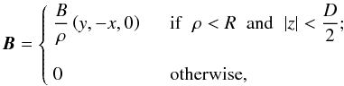 (2)with
  . To understand its effect, we first consider a particle moving in the YZ (x = 0) plane with direction u (the case depicted in Fig. 1). When it enters the lens, the cosmic ray finds an orthogonal magnetic field that curves its trajectory. The particle then rotates clockwise2 around the axis uB = B / B, describing a circle of gyroradius rg = E / (ecB). The segment of the trajectory inside the lens has a length l ≈ D, so when it departs the total rotation angle α0 is
  (3)The direction of the particle after crossing the lens is then v = RB(α0)u. The angle α0 will be the only parameter required to describe the effect of this basic lens. An important point is that B and the Lorentz force change sign if the trajectory goes through y < 0. In that case the deflection is equal in modulus but opposite to the one experience by particles going through y > 0 (see Fig. 1). Therefore, the effect of this lens is convergent, and all trajectories are deflected the same angle α0 towards the axis of the lens. The lens changes to divergent for particles of opposite electric charge or for particles reaching the lens from the opposite (z < 0) side.
The effect on a generic trajectory within a plane not necessarily orthogonal to the lens is a bit more involved. It is convenient to separate  (4)where u∥ = (u·uB)uB and u⊥ = u − u∥ are parallel and orthogonal to the magnetic field, respectively (and analogously for v). In this case the magnetic field will rotate the initial direction u an angle of α = u⊥α0 around the axis uB: v = RB(u⊥α)u. This means that the parallel components of the initial and the final directions coincide,
 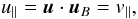 (5)whereas the orthogonal component u⊥, of modulus
  , rotates into
  (6)An important observation concerns the chromatic aberration of the lens. The deviation α0 caused by a given CML is proportional to the inverse energy of the cosmic ray. If E is small and α0 > π / 2, then the lens acts randomly on charged particles, diffusing them in all directions. On the other hand, if E is large the deviation becomes small and is smeared out as the particle propagates to the Earth. Only a region of the cosmic-ray spectrum can see the CML.
3. Image of a point-like source
We now study the image of a localized monochromatic source produced by the CML. We consider a thin lens (R ≫ D) located on the plane z = 0 (see Fig. 2). Its effect on a cosmic ray can be parametrized in terms of the angle α0 given in Eq. (3). The rotation axis is  (7)and the coordinates of source and observer are S = (s1,s2,s3) and O = (o1,o2,o3), respectively. We use the axial symmetry of the lens to set s1 = 0.
 |
Fig. 2 Trajectory from the source to the observer. |
 (8)
(8)
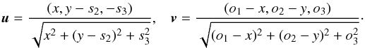
 |
Fig. 3 Trajectories with β > α (S1), β < α (S2) and β = 0 (S3) for an observer at the axis. |
 (9)The second one, derived from Eq. (6), defines the rotation of u⊥ produced by the magnetic field. It can be written as
 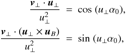 (10)where
  . The second equation above is necessary to fully specify the rotation. Notice that α = u⊥α0 has a definite sign: positive for a convergent CML and negative for a divergent one. In addition, the solution must verify that x2 + y2 < R2.
We find that, for R → ∞ and a convergent lens, there is always at least one solution, whereas for a divergent one there is a region around the axis that may be hidden by the CML. This region disappears if B goes smoothly to zero at the center of the lens. To illustrate the different possibilities in Fig. 3, we have placed the observer in the axis at a distance L from the lens, O = (0,0,−L), and parametrized the position of the source (at a distance d from the lens) as S = (0,dsinβ,dcosβ). In this case u∥ = 0 = v ∥ and u⊥ = 1. If the lens is convergent (α0 > 0) and | β | >α0, then the image of the source is just a single point. For a source at | β | <α0, we obtain two solutions, which correspond to trajectories from above or below the center of the lens. For a source in the axis (β = 0), the solution is a ring of radius  (11)If the observer is located out of the axis but still in the x = 0 plane the possibilities are similar, but the ring becomes a cross similar to the one obtained through gravitational lensing. Finally, if we take the observer out of the x = 0 plane, always appears a single solution.
4. Fluxes from distant sources
Finally we explore how the presence of a CML changes the flux F of charged particles from a localized source S. It is instructive to consider the case where S is a homogeneous disk of radius RS placed at a distance d from the lens and the observer O is at a large distance L,  (12)as shown in Fig. 4. In addition, we assume that the magnetic field defining the lens goes smoothly to zero near the axis and that the source is monochromatic.
If there were no lens, O would see S under a solid angle 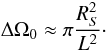 (13)If all the points on S are equally bright and the emission is isotropic, the differential flux dF / dΩ from all the directions inside the cone ΔΩ0 will be approximately the same, implying a total flux (number of particles per unit area)
  (14)The lens in front of S will deflect an approximate angle α all trajectories crossing far from the axis. In Fig. 4 we pictured3 the limiting directions reaching the observer, which define a cone
 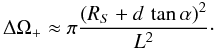 (15)Now O sees cosmic rays from directions inside the larger cone ΔΩ+ or, in other words, sees the radius RS of the source amplified to RS + d tanα.
 |
Fig. 4 Cone of trajectories from S to O with and without lens for a homogeneous and monochromatic source. |
We can then use Liouville’s theorem to deduce how the flux observed by O is affected by the presence of the lens. This theorem, first applied to cosmic rays moving inside a magnetic field by Lemaitre & Vallarta (1933), implies that an observer following a trajectory will always observe the same differential flux (or intensity, particles per unit area and solid angle) along the direction defined by that trajectory. For example, in the case with no lens an observer in the axis at a distance L′ ≫ L will still observe the same differential flux dF / dΩ. However, the cone of directions that he sees will be smaller,  , and the total flux from that source will scale like F′ ≈ F L2 / L′2. The effect of the lens is then just to change the cone of directions reaching O from S, without changing the differential flux. This implies an integrated flux
  (16)An important point is that the solid angle intervals ΔΩ0, + will in general be much smaller than the angular resolution at O. As a consequence, an observer trying to measure a differential flux will always include the whole cone ΔΩ0, + within the same solid angle bin: only the integrated fluxes F0, + (averaged over the angular resolution) are observable.
Now we suppose that there are many similar sources at approximately the same distance from the observer and covering a certain range of directions. Cosmic rays emitted from each source will reach O within a very tiny cone ΔΩ0 and will be observed integrated over that cone and averaged over the angular resolution. If one of the sources has a CML in front, its cone ΔΩ+ at O and thus its contribution to one of the direction bins will be larger, which would translate into a low-scale anisotropy4 within the range of directions covered by the sources (see Fig. 5, left).
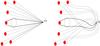 |
Fig. 5 Trajectories from S to O without (left) and with (right) irregular magnetic fields along the trajectory. |
In principle, this effect would not be erased by irregular magnetic fields from the source to the observer, which deflect the trajectories and tend to isotropize the fluxes (in Fig. 5, right). The contribution from the source behind the CML (reaching O now from a different direction) will still tend to be greater. The effect of the lens is to increase the size RS of the source to RS + d tanα. Random magnetic fields will change the direction of arrival and the effective distance between S and O (i.e., the direction and the size of the cone from each source), but neither the initial deflection produced by the lens nor (by Liouville’s theorem) the differential flux within each tiny cone. Therefore, the cone from the source behind the lens tends to be larger and, when integrated and averaged over the resolution bin, may still introduce a low-scale anisotropy. The effect, however, tends to vanish if the cones are so small that the probability of observing two particles from the same cone of directions is lower than the probability of observing particles from two disconnected cones with origins in the same source (i.e., in the deep diffuse regime where trajectories become random walks).
Finally, the effect of a divergent CML would be just the opposite. The presence of a lens could then introduce an excess for positively charged particles and a defect for the negative ones (or a matter-antimatter asymmetry if both species were equally emitted by S).
5. Summary and discussion
It is known that galactic and intergalactic magnetic fields play a very important role in the propagation of charged cosmic rays. Here we have explored the effect of a very simple configuration, a constant azimuthal field in a thin disk, which we identify as a CML. Such an object acts on cosmic rays like a gravitational lens on photons, with some very interesting differences. Gravitational lenses are always convergent, whereas if a magnetic lens is convergent for protons and positrons, it changes to divergent for antiprotons and electrons. In addition, the deflection that the CML produces depends on the particle energy, so the lense is only visible in a definite region of the spectrum.
Our intention has been to introduce the concept of CML and discuss its possible effects, leaving the search for possible candidates to future work. Generically, the magnetic-field configuration defining the CML is natural and tends to be established by the dynamo effect. For example, in spiral galaxies, B can be purely azimuthal (the one we have assumed), axisymmetric spiral, or bisymmetric spiral, with or without reversals (Beck 2005; Battaner et al. 2008), but in all cases the azimuthal component dominates. Our galaxy is not an exception (Han 2010; Ruiz et al. 2009), it includes a spiral magnetic field of B ≈ 4 μG in the disk. This would actually force any analysis of magnetic lensing by other galaxies to subtract the effect produced by our own magnetic field. CMLs could also be present in galactic halos, as there are observations of polarized synchrotron emission that suggest the presence of regular fields (Dettmar et al. 2006). Analogous indications (Bonafede et al. 2009) can be found for larger structures, such as clusters and their halos. Inside our galaxy, the antisymmetric tori placed 1.5 kpc away in both hemispheres discovered by Han et al. (1997) would also produce magnetic lensing on ultrahigh energy cosmic rays. At lower scales (20–800 pc) molecular clouds and HII regions (Gonzalez et al. 1997) are also potential candidates. Molecular clouds have strong regular fields in the range of 0.1–3 mG (Crutcher 2005). Moreover, many reversals in the field direction observed in our galaxy seem to coincide with HII regions (Wielebinski 2005), which would indicate that the field follows the rotation velocity in that region. There are also observations of Faraday screens covering angles of a few minutes of unknown origin (Mitra et al. 2003). Finally, nearby protostellar disks may provide a magnetic analog to the gravitational microlenses, because they define small objects of ≈103 AU diameter with azimuthal magnetic fields (Stepinski 1995) of order tens of mG (Goncalves et al. 2008). Therefore, we think it is justified to presume that CMLs may appear on any scales R with different values of B.
The lensing produced by a CML will be affected by the turbulent magnetic fields, but they should remain observable under certain conditions. For example, the typical lensing produced by a galaxy on cosmic rays of energy above 109 GeV is caused by a regular magnetic field on the order of μG, while the distortions will come from similar fluctuations. The region of coherence of these magnetic fluctuations, however, is just around 10–100 pc, varying randomly from cell to cell. Since the regular field that defines the lens will act along 10–100 times greater distances, its effect on cosmic rays will dominate, and the expected blurring due to turbulences will be small. For CMLs inside our galaxy, one should in general subtract the effect of the local field on the relevant scale. Suppose, for example, that we have a small lens (D ≈ 10-3 pc) with a strong magnetic field (B ≈ 1 mG) at a distance below 10 pc from the Earth. If the magnetic field along the trajectory from the lens to the Earth is μG (with weaker turbulences on smaller scales), then the effects of the lens on 106 GeV cosmic rays can be observed, but from a displaced direction. In any case, the identification of a CML would require a detailed simulation that includes a full spectrum of magnetic turbulences.
We studied the image of a point-like source and find interesting patterns that are the analogous to the gravitational Einstein ring and Einstein cross. Here the effect would be combined with a strong chromatic dependence, as the deviation is proportional to the inverse energy of the particle. The images would be absent (or placed in a different location) for particles of opposite charges, since they would find a divergent lens. We also studied the effect of a CML on the flux from a localized source. If the source and the lens are far from the observer (i.e., if it covers a small solid angle), it seems possible to generate small-scale anisotropies.
A continuous field configuration could be modeled just by adding a factor of (1 − exp[(ρ / ρ0)n0]) × exp[(ρ / R)nR] × exp[(2z / D)nD]. When the integers n0, nR, and nD are chosen very large and ρ0 very small, we recover our disk with a null B at ρ = 0.
We define a positive deviation α0 if the rotation from u to v around the axis uB is clockwise.
A pointlike source in the axis is transformed by the lens into a ring, as explained in Sect. 4. As the source grows, the ring becomes thicker and eventually closes to a circle, which is the case considered in Fig. 4.
The direction of the source would be measured with a Gaussian distribution that could take it to adjacent bins.
Acknowledgments
This work has been funded by MICINN of Spain (AYA2007-67625-CO2-02, FPA2006-05294, FPA2010-16802, and Consolider-Ingenio Multidark CSD2009-00064) and by the Junta de Andalucía (FQM-101/108/437/792).
References
- Battaner, E., Florido, E., Guijarro, A., et al. 2008, in Lecture Notes and Essays in Astrophysics, 3, 83 [NASA ADS] [Google Scholar]
- Beck, R. 2005, in Cosmic Magnetic Fields, ed. by R. Beck, & R. Wielebinski (Springer Verlag), 41 [Google Scholar]
- Bonafede, A., Feretti, L., & Giovannini, G. 2009, A&A, 503, 707 [NASA ADS] [CrossRef] [EDP Sciences] [Google Scholar]
- Brandenburg, A., & Subramanian, K. 2005, Phys. Rep., 417, 1 [NASA ADS] [CrossRef] [Google Scholar]
- Crutcher, R. M. 2005, in Magnetic Fields in the Universe: from Laboratory and Stars to the Primordial Structures, ed. E. M. de Gouveia dal Pino, et al., AIP Conf. Proc., 784, 129 [Google Scholar]
- Dettmar, R. J., & Soida, M. 2006, Astron. Nachr., 327, 495 [Google Scholar]
- Dolag, K., Kachelriess, M., & Semikoz, D. V. 2009, JCAP, 0901, 033 [NASA ADS] [Google Scholar]
- Goncalves, J., Galli, D., & Girart, J. M. 2008, A&A, 490, 39 [Google Scholar]
- González-Delgado, R., & Pérez, E. 1997, ApJS, 108, 1 [NASA ADS] [CrossRef] [Google Scholar]
- Han, J. L. 2009, in Cosmic magnetic fields: from planets to stars and galaxies, IAU Conf. Proc., 259, 455 [Google Scholar]
- Han, J. L., Manchester, R. N., Berkhuijsen, E. M., & Beck, R. 1997, A&A, 352, 98 [NASA ADS] [Google Scholar]
- Harari, D., Mollerach, S., & Roulet, E. 2001, in Observing ultrahigh energy cosmic rays from space and Earth, AIP Conf. Proc., 566, 289 [Google Scholar]
- Harari, D., Mollerach, S., & Roulet, E. 2005, in Magnetic Fields in the Universe: from Laboratory and Stars to Primordial Structures, AIP Conf. Proc., 784, 763 [NASA ADS] [CrossRef] [Google Scholar]
- Harari, D., Mollerach, S., & Roulet, E. 2010, J. Cosmol. and Astropart. Phys., 11, 033 [NASA ADS] [CrossRef] [Google Scholar]
- Lemaitre, G., & Vallarta, M. S. 1933, Phys. Rev. 43, 87 [NASA ADS] [CrossRef] [Google Scholar]
- Mitra, D., Wielebinski, R., Kramer, M., & Jessner, A. 2003, A&A, 398, 993 [NASA ADS] [CrossRef] [EDP Sciences] [Google Scholar]
- Parker, E. 1971, ApJ, 163, 279 [NASA ADS] [CrossRef] [Google Scholar]
- Ruiz-Granados, B., Rubiño-Martín, J. A., & Battaner, E. 2009, in Cosmic magnetic fields: from planets to stars and galaxies, IAU Conf. Proc. 259, 573 [Google Scholar]
- Shaviv, N. J., Heyl, J. S., & Lithwick, Y. 1999, MNRAS, 306, 333 [NASA ADS] [CrossRef] [Google Scholar]
- Stepinski, T. F. 1995, Rev. Mex. Astron. Astrophys. 1, 267 [NASA ADS] [Google Scholar]
- Wielebinski, R. 2005, in The Magnetized Plasma in Galactic Evolution, ed. K. Chyzy, et al., Jagiellonian Univ. Krakow, Proc. Conf., 125 [Google Scholar]
All Figures
|
Fig. 1 Trajectories in the x = 0 plane. B ∝ (1,0,0) at y > 0 and B ∝ (−1,0,0) at y < 0. |
| In the text | |
|
Fig. 2 Trajectory from the source to the observer. |
| In the text | |
|
Fig. 3 Trajectories with β > α (S1), β < α (S2) and β = 0 (S3) for an observer at the axis. |
| In the text | |
|
Fig. 4 Cone of trajectories from S to O with and without lens for a homogeneous and monochromatic source. |
| In the text | |
|
Fig. 5 Trajectories from S to O without (left) and with (right) irregular magnetic fields along the trajectory. |
| In the text | |
Current usage metrics show cumulative count of Article Views (full-text article views including HTML views, PDF and ePub downloads, according to the available data) and Abstracts Views on Vision4Press platform.
Data correspond to usage on the plateform after 2015. The current usage metrics is available 48-96 hours after online publication and is updated daily on week days.
Initial download of the metrics may take a while.