| Issue |
A&A
Volume 527, March 2011
|
|
|---|---|---|
| Article Number | A61 | |
| Number of page(s) | 14 | |
| Section | Interstellar and circumstellar matter | |
| DOI | https://doi.org/10.1051/0004-6361/201015624 | |
| Published online | 25 January 2011 | |
Dust formation in the ejecta of the type II-P supernova 2004dj
1
Department of Optics and Quantum ElectronicsUniversity of
Szeged,
Dóm tér 9.,
6720
Szeged,
Hungary
e-mail: szaszi@titan.physx.u-szeged.hu; vinko@titan.physx.u-szeged.hu
2
Max-Planck-Institut für Astronomie, Kőnigstuhl 17, 69117
Heidelberg,
Germany
3
Steward Observatory, University of Arizona,
Tucson,
AZ
85721,
USA
4 Konkoly Observatory of the Hungarian Academy of Sciences,
1525 Budapest, PO Box 67, Hungary
5 Sydney Institute for Astronomy, School of Physics A28,
University of Sydney, NSW 2006, Australia
Received:
22
August
2010
Accepted:
9
December
2010
Aims. Core-collapse supernovae (CC SNe), especially type II-Plateau ones, are thought to be important contributors to cosmic dust production. SN 2004dj, one of the closest and brightest SN since 1987A, offered a good opportunity to examine dust-formation processes. To find signs of newly formed dust, we analyze all available mid-infrared (MIR) archival data from the Spitzer space telescope.
Methods. We re-reduced and analyzed data from IRAC, MIPS, and IRS instruments obtained between +98 and +1381 days after explosion and generated light curves and spectra for each epoch. Observed spectral energy distributions are fitted with both analytic and numerical models, using the radiative-transfer code MOCASSIN for the latter ones. We also use imaging polarimetric data obtained at +425 days by the Hubble space telescope.
Results. We present convincing evidence of dust formation in the ejecta of SN 2004dj from MIR light curves and spectra. Significant MIR excess flux is detected in all bands between 3.6 and 24 μm. In the optical, a ~0.8% polarization is also detected at a 2-sigma level, which exceeds the interstellar polarization in that direction. Our analysis shows that the freshly-formed dust around SN 2004dj can be modeled assuming a nearly spherical shell that contains amorphous carbon grains, which cool from ~700 K to ~400 K between +267 and +1246 days. Persistent excess flux is found above 10 μm, which is explained by a cold (~115 K) dust component. If this cold dust is of circumstellar origin, it is likely to be condensed in a cool, dense shell between the forward and reverse shocks. Pre-existing circumstellar dust is less likely, but cannot be ruled out. An upper limit of ~8 × 10⁻⁴ M⊙ is derived for the dust mass, which is similar to previously published values for other dust-producing SNe.
Key words: supernovae: general / supernovae: individual: SN 2004dj / dust, extinction
© ESO, 2011
1. Introduction
Core-collapse supernovae (CC SNe) are usually interpreted as the endpoints in the life cycle of massive stars (M ≳ 8 M⊙, e.g. Woosley et al. 2002). While it is widely accepted that these high-energy events have significant effects on the birth and evolution of other stars, there has been a long-standing argument whether they also play an important role in the formation of interstellar dust.
Theories on the dust-production of CC SNe have been around for over 40 years (Cernuschi et al. 1967; Hoyle & Wickramasinghe 1970). These early hypotheses were later supported by studies of isotopic anomalies in meteorites (Clayton 1979; Clayton et al. 1997; Clayton & Nittler 2004). Additionally, several papers were published about the unexpectedly large dust content of high-redshift galaxies (Pei et al. 1991; Pettini et al. 1997; Bertoldi et al. 2003), which suggested that CC SNe could be the main sources of interstellar dust in the early (and maybe in the present) Universe (Todini & Ferrara 2001; Nozawa et al. 2003; Morgan & Edmunds 2003). The average lifetimes of CC SNe are short enough to produce dust at high redshifts, i.e. during ~1 Gyr, thus these SNe are better candidates for explaining the presence of early dust than other possible sources, like AGB stars (e.g. Dwek et al. 2007).
Although these theories have not been disclaimed so far, there are several other possible mechanisms of dust formation in distant galaxies. Valiante et al. (2009) showed that different star-formation histories of galaxies should be taken into account to avoid underestimating the contribution of AGB stars to the whole dust production. Another possibility is the condensation of dust grains in quasar winds (Elvis et al. 2002), which has also been supported by observations (Markwick-Kemper et al. 2007). On the other hand, there are many high-z galaxies where SN-explosions are the only viable explanation for the observed amount of dust (Maiolino et al. 2004; Stratta et al. 2007; Michalowski et al. 2010). Detailed studies by Matsuura et al. (2009) suggest a “missing dust-mass problem” in the Large Magellanic Cloud (LMC), similar to the situation in distant galaxies described above.
The two main problems with the observable dust content around SNe are the amount and the origin. Models of Kozasa et al. (1989), Todini & Ferrara (2001), and Nozawa et al. (2003) predict 0.1−1 M⊙ of newly formed dust after a CC SN event. More recently, Bianchi & Schneider (2007), Kozasa et al. (2009), and Silvia et al. (2010) have found similar values via numerical modeling of the survival of dust grains. They have found that the dust amount depends on the type of SN and also the density of the local ISM, which must be taken into account when estimating the contribution of CC SNe to the dust content in high-redshift galaxies.
Despite the nearly concordant results of different models, direct observations have not confirmed the massive dust production by CC SNe yet (although a detailed analysis was possible only in a few cases). The first evidence for dust condensation was observed in SN 1987A (e.g. Danziger et al. 1989, 1991; Lucy et al. 1989, 1991; Roche et al. 1993; and Wooden et al. 1993; revisited by Ercolano et al. 2007). The observed signs of dust formation were i) a strong decrease of optical fluxes around 500 days after explosion; ii) an increase of mid-infrared (MIR) fluxes at the same time; and iii) increasing blueshift and asymmetry of the optical emission lines because of an attenuation of the back side of the ejecta by the freshly synthesized dust. The mass of newly condensed dust was estimated to be ~10-4 M⊙. Similar effects were also detected in the ejecta of type II-P SN 1999em and type Ib/c SN 1990I (Elmhamdi et al. 2003, 2004).
The launch of the Spitzer space telescope (hereafter Spitzer) in 2003 and AKARI in 2006 provided additional opportunities to observe dust around CC SNe by following the evolution of MIR light curves and spectra. Evidence for newly condensed dust were obtained for SN 2003gd (Sugerman et al. 2006; Meikle et al. 2007), 2004et (Kotak et al. 2009), 2007od (Andrews et al. 2010), and type Ib/c SN 2006jc (Nozawa et al. 2008; Mattila et al. 2008; Tominaga et al. 2008; and Sakon et al. 2009). In every case, the estimated mass of recently formed dust was between 10-5−10-3 M⊙. Note that for SN 2003gd Sugerman et al. (2006) calculated a value of 0.02 M⊙, but their result was questioned by Meikle et al. (2007). These values are significantly lower than the theoretically predicted ones and tend not to support an SN origin for observable amounts of dust in the local and distant universe.
There are other ways to discover dust around SNe. As it was found in some CC SNe (e.g. SN 1998S, Pozzo et al. 2004; SN 2005ip, Smith et al. 2009; and Fox et al. 2009; SN 2006jc, Smith et al. 2008a; SN 2006tf, Smith et al. 2008b; SN 2007od, Andrews et al. 2010), dust grains may condense in a cool dense shell (CDS) that is generated between the forward and reverse shock waves during the interaction of the SN ejecta and the pre-existing circumstellar medium (CSM). The CDS may affect both the light curves and the spectral line profiles. Another possibility is the thermal radiation of pre-existing dust in the CSM that is re-heated by the SN as an IR-echo (Bode & Evans 1980; Dwek 1983, 1985; Sugerman 2003), which can be observed as an infrared excess (e.g. SN 1998S, Gerardy et al. 2002; Pozzo et al. 2004; SN 2002hh, Barlow et al. 2005; Meikle et al. 2006; SN 2006jc, Mattila et al. 2008; SN 2004et, Kotak et al. 2009; SN 2008S, Botticella et al. 2009). These results seem to support the hypothesis that pre-explosion mass-loss processes of progenitor stars could play a more important role in dust formation than the explosions of CC SNe (see also Prieto et al. 2008; and Wesson et al. 2010).
Recent studies of SN remnants (SNRs) could not solve the question of the amount of dust produced by SNe. By obtaining far-IR and sub-mm observations, many groups estimated the amount of newly condensed dust grains in Cas A (Dunne et al. 2003; Krause et al. 2004; Rho et al. 2008). Their results varied between 0.02 and 2 M⊙, while the values for Kepler SNR showed an even larger discrepancy (0.1−3 M⊙ by Morgan et al. 2003; and 5 × 10⁻⁴ M⊙ by Blair et al. 2007). Stanimirovic et al. (2005) and Sandstrom et al. (2009) studied the MIR data of SNR 1E0102.2-7219 in the Small Magellanic Cloud (SMC) and found evidence for ~1−3 × 10⁻³ M⊙ of dust formed in the ejecta (the authors of the latter paper also calculated that the amount of cold dust that is observable only at longer wavelengths could be even higher by two orders of magnitude).
Estimating the mass of dust around SNe is complicated, and the results are strongly model-dependent. Several ideas have been proposed to explain the discrepancies between observations and theory. Using clumpy grain-density distributions (Sugerman et al. 2006; Ercolano et al. 2007) leads to a dust mass in a SN ejecta at least one order of magnitude higher than by assuming a smooth density distribution. Regarding dust enrichment in high-z galaxies, the low dust production rates of observed CC SNe might be compensated by using a top-heavy initial mass function (IMF), resulting in more SNe per unit stellar mass (Michalowski et al. 2010, and references therein). It is also a possibility that SN explosions provide only the dust seeds, while the bulk of the dust mass is accumulated during grain growth in the ISM (Draine 2003, 2009; Michalowski et al. 2010, and references therein). It has also been noted that estimates of the dust content at high redshifts should be considered with caution because of the uncertainties in interpreting low signal-to-noise observations (see e.g. Zafar et al. 2010).
The aim of this paper is to study the dust formation in the nearby bright type II-P SN 2004dj. This SN occured in the compact cluster Sandage-96 (S96) in NGC 2403, and owing to its proximity (~3.5 Mpc, Vinkó et al. 2006) it has been intensively studied since the discovery by Itagaki (Nakano et al. 2004; Patat et al. 2004). Early observations have been summarized by Vinkó et al. (2006, hereafter Paper I), while the physical properties of S96 have been recently discussed by Vinkó et al. (2009, hereafter Paper II). The progenitor was identified as a massive (12 M⊙ ≲ Mprog ≲ 20 M⊙) star within S96 (Maíz-Apellániz et al. 2004; Wang et al. 2005; Paper II).
The evolution of SN 2004dj was extensively observed by Spitzer. The earliest observations have been presented by Kotak et al. (2005). In the following sections we analyze the Spitzer and Hubble observations that show signs of dust formation (Sects. 2 and 3), then we compare various dust models with these observations in Sect. 4. Finally, we present our conclusions in Sect. 5.
2. Observations and data reduction
This section contains the description of the Spitzer- and Hubble observations that we use to probe the newly formed dust in SN 2004dj. Throughout this paper we adopt JD 2 453 187.0 (2004-06-30) as the moment of explosion (see Paper I).
2.1. MIR Photometry with Spitzer
We collected all public archival Spitzer data on SN 2004dj for each channel (3.6, 4.5, 5.8 and 8.0 μm) of the Infrared Array Camera (IRAC) and for the 24 μm channel of the Multiband Imaging Spectrometer (MIPS). We use all available basic- and post-basic calibrated data (BCD and PBCD) obtained from +98 to +1381 days past explosion (summarized in Table 1).
 |
Fig. 1 Post-BCD images showing the environment of SN 2004dj obtained with Spitzer on 2004-10-12: IRAC 3.6 micron (top left), 5.8 micron (top right), 8.0 micron (bottom left), and MIPS 24.0 micron (bottom right). The SN is marked in each panel. The target is very faint on the MIPS image, which illustrates the necessity of PSF-photometry (see text for details). |
The IRAC BCD images were processed using the IRACproc software (Schuster et al. 2006) to create final mosaics with a scale of 0.86′′/pixel. Aperture photometry was also carried out with this package (which uses built-in IRAF1 scripts) with an aperture radius 2′′ and a background annulus from 2′′ to 6′′. Aperture corrections of 1.213, 1.234, 1.379, and 1.584 were used for channels 1–4, respectively (Table 5.7 in IRAC Data Handbook, Reach et al. 2006). We compared our results against aperture photometry on PBCD images using the IRAF phot task with the same parameters, and found a reasonably good agreement.
Registration, mosaicing and resampling of the MIPS images were made by using the DAT software (Engelbracht et al. 2007). The source was not detected on the 70 μm images, therefore we analyzed only the 24 μm frames. The photometry of the 24 μm data was complicated, because the source was very faint, peaking only slightly above background (see Fig. 1). First, aperture photometry was performed on the 1.245′′/pixel scale mosaics using an aperture radius of 3.5′′ and a background annulus from 6′′ to 8′′. An aperture correction of 2.78 was then applied (Engelbracht et al. 2007). The choice of such a small aperture and annulus was motivated by the close, bright H ii region, which makes the background high and variable on one side of the source.
Second, PSF-photometry was carried out on the 24 μm MIPS frames using a
custom-made empirical PSF (assembled from multiple epoch observations of HD 173398) using
IRAF/DAOPHOT. We set the PSF radius as 90 pixels, for which no computed
aperture correction is available. Therefore, the photometric calibration was done by
comparing the results of the properly calibrated aperture photometry and our
PSF-photometry for two isolated point-like sources within the SN-field that do not suffer
from the contamination of a nearby bright object. We compared the the sum of the count
rates on the DAT frames (in DN/s) from both aperture- and PSF-photometry,
aperture-corrected the numbers from aperture photometry and found the following linear
relationship betweeen the aperture-corrected count rates
(fapcor) and those from our
PSF-photometry (fPSF):
 (1)The fluxes from
PSF-photometry corrected this way were then converted to mJy as prescribed for MIPS and
found to be within the errors of those from aperture photometry.
(1)The fluxes from
PSF-photometry corrected this way were then converted to mJy as prescribed for MIPS and
found to be within the errors of those from aperture photometry.
We also performed PSF-photometry with the IDP3 software (Stobie & Ferro 2006), which agreed well with the results of DAOPHOT. As a triple-check, we also performed aperture photometry on the PBCD-images and found reasonable agreement between the absolute flux levels computed from PSF- and aperture photometry. Thus, the final 24 μm fluxes were calculated as the average of the results from the different methods. The final photometry of SN 2004dj is collected in Table 1. The errors represent the standard deviation of the data from the three different photometry methods.
Kotak et al. (2005) presented some MIR photometric points observed at ~100 days after explosion. Their reported flux values are generally consistent with ours, but there are some differences (mainly in channels 4.5 and 24 μm). The reason for these minor differences may be that they applied larger aperture radii (3.6′′ and 5.6′′ for 4.5 and 24 μm data, respectively) and performed only aperture photometry on the PBCD images.
Spitzer photometry for SN 2004dj.
2.2. MIR Spectroscopy with IRS
SN 2004dj was observed with the Infrared Spectrograph (IRS) onboard Spitzer on seven epochs between October 2004 and November 2006, from +115 to +868 days after explosion. These observations were made in the IRSStare mode using the Short-Low (SL) setup. Table 2 contains the list of spectroscopic data downloaded from the Spitzer archive. In addition, several imaging observations were made with the blue array (16 μm central wavelength) of the peak-up imaging (PUI) mode of IRS, which are listed in Table 1.
We analyzed the PBCD-frames containing the spectroscopic data using the SPitzer IRS Custom Extraction software (SPICE2). Sky subtraction and bad pixel removal were performed using two exposures containing the spectrum at different locations, and subtracting them from each other. Order extraction, wavelength- and flux-calibration were performed applying built-in templates within SPICE. Finally, the spectra from the 1st, 2nd and 3rd orders were combined into a single spectrum with the overlapping edges averaged. In a few cases the sky near the order edges was oversubtracted because of excess flux close to the source, which resulted in spurious negative flux values in the extracted spectrum. These were filtered out using the fluxes in the same wavelength region that were extracted from the adjacent orders. The results were also checked by comparing the extracted fluxes with photometry (Table 1). Reasonable agreement between the spectral and photometric fluxes was found for all spectra.
The final calibrated and combined spectra cover the 5.15−14.23 μm wavelength regime with resolving power R ~ 100. These are plotted in Fig. 2, where a small vertical shift is applied between the spectra for better visibility. The analysis of the spectral features and evolution will be presented in Sect. 3.
The fluxes of SN 2004dj in the PUI frames were measured via aperture photometry by the MOsaicker and Point source EXtractor (MOPEX3) software. The results are given in Table 1. These broad-band integrated fluxes were only used for checking the shape of the SED between the IRAC and MIPS bands, but were not included in the detailed analysis in Sect. 3.
IRS observations of SN 2004dj.
Identified lines in the IRS spectra of SN 2004dj.
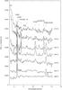 |
Fig. 2 IRS spectra of SN 2004dj in the nebular phase. Line identification is based on Kotak et al. (2005, 2006). The evolution of the features is discussed in Sect. 3.2. |
2.3. Imaging polarimetry with HST
SN 2004dj and its surrounding cluster, Sandage-96, were imaged by HST/ACS High-Resolution Camera (HRC) on 2005 Aug. 28 (proposal GO-10607, PI: B.E.K. Sugerman), +425 days after explosion. Among others, three sets of four drizzled frames were recorded through the F435W filter at 0, 60, and 120 degree position of the POLUV polarization filter (see Paper II for the description and analysis of all observations). Here we consider only the polarization measurement of the SN.
We measured the flux from SN 2004dj with PSF-photometry using the DOLPHOT
software (Dolphin 2000) the same way as
described in Paper II. From the fluxes measured at three different polarizer angles
(I0, I60 and
I120), the Stokes-parameters (I,
Q, U) were calculated applying the formulae given by
e.g. Sparks & Axon (1999). The
degree-of-polarization, p was then derived as
 (2)This resulted in a
measured degree-of-polarization p = 0.0941 ± 0.0029, which is, of course,
much higher than the true p from SN 2004dj, owing to instrumental
polarization (pi), and the polarization from
interstellar matter (pISM).
(2)This resulted in a
measured degree-of-polarization p = 0.0941 ± 0.0029, which is, of course,
much higher than the true p from SN 2004dj, owing to instrumental
polarization (pi), and the polarization from
interstellar matter (pISM).
The instrumental polarization of ACS was studied by Biretta et al. (2004). Using three sets of in-orbit calibration data they measured the instrumental polarization as pi = 0.086 ± 0.002 for the ACS/HRC+F435W+POLUV detector+filter combination (see their Table 20). They also give a semi-empirical formula describing the relative uncertainty of the degree-of-polarization, σp/p, as a function of the signal-to-noise of the flux measurement.
Adopting this calibration, the measured true degree-of-polarization, corrected for the instrumental zero-point, is ptrue = 0.0081 ± 0.0036. The average S/N of the three flux measurements for SN 2004dj is ~200, from which we derived σp/p = 0.5588, thus, σp = 0.0045, which agrees well with the error estimate of ptrue given above.
Further analysis and discussion of the polarization data are presented in Sect. 3.
3. Analysis of the observations
3.1. The effect of the surrounding cluster Sandage-96
The bright, compact cluster S96 surrounding SN 2004dj (Paper II) made late-time optical measurements difficult, because the light from the cluster stars contribute significantly to the total measured fluxes. This was very problematic in the optical, but fortunately less severe in the MIR, where the cluster is much fainter. Although we have no pre-SN MIR photometry for S96, we estimated its MIR flux using the best-fitting cluster models from Paper II. These models are simple, coeval stellar populations (SSP), but we considered three different model sets using different input physics to test the model dependence of the flux predictions.
Figure 3 illustrates the MIR SEDs for the three SSP models that produced the best fit to the observed UV+optical+NIR data of S96 (Fig. 3 filled symbols; see Paper II for details). Fortunately, the three models predicted very similar MIR fluxes in the Spitzer bands. Their average values (in cgs units) are collected in Table 4, where the errors illustrate the flux differences between the models.
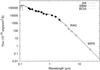 |
Fig. 3 Best-fitting model SEDs for the host cluster Sandage-96 from Paper II. Filled circles represent observed data for the cluster, while open symbols denote the averaged MIR-fluxes from the models (see Table 4). |
Evidently the cluster contributes significantly to the measured SN fluxes only in the IRAC channels, but the cluster flux drops below the observational uncertainties longward of 10 μm. Thus, we subsequently corrected the IRAC fluxes for this offset using the model fluxes from Table 4, but this correction was not necessary for the PUI and MIPS data.
3.2. Spectral features and evolution
The nebular spectra of SN 2004dj presented in Fig. 2 are typical for type II-P SNe. They show features and evolution very similar to the available MIR spectra of a few SNe, including SN 1987A (Wooden et al. 1993; Roche et al. 1993), SN 2005af (Kotak et al. 2006) and SN 2004et (Kotak et al. 2009). The first two spectra of SN 2004dj (taken at +115 d and +139 d) have been already presented and discussed by Kotak et al. (2005). We include these spectra in the present study for completeness, but the conclusions for them are generally the same as those of Kotak et al. (2005).
Contribution of the Sandage-96 cluster to the MIR fluxes of SN 2004dj.
The spectra consist of permitted emission lines of H i (Pfund-, Humphrey- and n = 7 series), and forbidden lines of [Ni i], [Ni ii], [Co ii] and [Ar ii]. Table 3 summarizes the identified lines, based on Wooden et al. (1993) and Kotak et al. (2005). The presence of [Ne ii], forming a blend with [Ni ii] at 12.8 μm, was suggested by Kotak et al. (2006) for SN 2005af. This feature is also present in SN 2004dj for all phases covered by IRS-observations, although the two components cannot be resolved.
The blue edge of the first two spectra is influenced by the red wing of the 1−0 vibrational transition of the CO-molecule, similar to SN 1987A, as first pointed out by Kotak et al. (2005). CO 1−0 remained detectable in the two subsequent spectra up to +291 days. No sign of the SiO fundamental band around 8 μm was detected in SN 2004dj, unlike in SNe 1987A, 2005af and 2004et. Because we present evidence that SN 2004dj showed significant dust formation after +400 days, the absence of detectable SiO can be an important constraint for the chemical composition of the newly formed dust grains.
3.3. Masses of Ni and Co
Masses of freshly synthesized Ni estimated from observations may provide important
constraints for SN explosion models (e.g. Woosley & Weaver 1995; Thielemann et al. 1996;
Chieffi & Limongi 2004; Nomoto et al. 2006). Following the methods presented in Roche et al.
(1993) and Wooden et al. (1993), we derived the ionization fraction of stable 58Ni
from the measured ratio of fluxes of the collisionally-excited lines of [Ni ii]
at 6.63 μm and [Ni i] at 7.51 μm. It was shown
by Wooden et al. (1993) and Kotak et al. (2005) that the critical density (at which the
collisional de-excitation rate equals the rate of spontaneous decay) for the
6.63 μm line is ~1.3 × 107 cm-3, while the
electron density ~1 year after explosion is ~108 cm-3, one order
of magnitude higher, making LTE-conditions valid. Under these conditions the total number
of excited atoms at the upper level u of the given transition can be
expressed as  (3)where
D is the distance to the SN (3.5 Mpc, Paper I),
Ful is the measured line flux (in erg
s-1 cm-2), λ is the wavelength of the transition
and Aul is the transition probability
(in cm-1). Note that this expression is valid for optically thin lines, but
the [Ni ii] 6.63 μm feature was probably optically thick between
100 − 660 days (Wooden et al. 1993). Thus, the
derived quantities for this line are actually lower limits. The ratio of the total number
of neutral Ni0 and ionized Ni+ can be obtained from the ratio of
measured line fluxes via Boltzmann- and Saha-equations.
(3)where
D is the distance to the SN (3.5 Mpc, Paper I),
Ful is the measured line flux (in erg
s-1 cm-2), λ is the wavelength of the transition
and Aul is the transition probability
(in cm-1). Note that this expression is valid for optically thin lines, but
the [Ni ii] 6.63 μm feature was probably optically thick between
100 − 660 days (Wooden et al. 1993). Thus, the
derived quantities for this line are actually lower limits. The ratio of the total number
of neutral Ni0 and ionized Ni+ can be obtained from the ratio of
measured line fluxes via Boltzmann- and Saha-equations.
It is important that the 7.51 μm line in the IRS
spectra is an unresolved blend of [Ni i] with Paα,
Huβ and H i 7-11, which makes the direct measurement of the
[Ni i] feature difficult. This was already noted by Kotak et al. (2005), but in a subsequent paper Kotak et al. (2006) measured the flux of this line directly and
derived the ionization fraction x = Ni+/(Ni0 +
Ni + ) ~ 0.4 for SN 2004dj at +261 days. This is roughly a factor of 2 lower
than what was measured in SN 1987A at that epoch (x ~ 0.8, Wooden et al.
1993). In order to clarify this, we estimated the
line flux of the [Ni i] feature assuming that the H i features have the
same ratio to the total line flux as was measured by Wooden et al. (1993) for SN 1987A in higher resolution spectra. The contribution from
H i was found to be as high as 90 percent at +260 days, which decreased to 75
percent at +450 days and less than 10 percent at +660 days. We used these numbers to
estimate the [Ni i] fluxes from the measured total line fluxes (the
[Ni ii] 6.63 μm feature was not affected by this
complication). The results are collected in Table 5. Using these line fluxes and assuming Te = 3000 K
electron temperature (Wooden et al. 1993), the
ionization fraction was computed as
![\begin{eqnarray} y &=& {N({\rm Ni^+}) \over N({\rm Ni^0})} \nonumber \\ &=&\!{F(6.63) \over F(7.51)}\! {6.63 \over 7.51} \!{ {g_{7.51} A_{7.51}} \over {g_{6.63} A_{6.63}}}\! {z^{+}(T_{\rm e}) \over z^{0}(T_{\rm e})} \exp[(E_{6.63}\!-\!E_{7.51})/kT_{\rm e}], \end{eqnarray}](/articles/aa/full_html/2011/03/aa15624-10/aa15624-10-eq82.png) (4)then
applying
x = y/(1 + y),
where g is the statistical weight,
z + ,0(T) are the
partition functions for ionized and neutral Ni, respectively, and E is
the excitation potential for the upper level of the given transition. The values of the
atomic parameters were adopted from the NIST Atomic Spectral Database4. The derived ionization fractions are shown in the last column of
Table 5. These values are very close to those
obtained by Wooden et al. (1993) for SN 1987A, but
significantly higher than the results by Kotak et al. (2006). It is probable that Kotak et al. overestimated the contribution of
[Ni i] to the 7.51 μm feature, and therefore underestimated
the ionization fraction for Ni. Our new result suggests that the Ni ionization and
probably other physical conditions in the ejecta of SN 2004dj were quite similar to those
in SN 1987A.
(4)then
applying
x = y/(1 + y),
where g is the statistical weight,
z + ,0(T) are the
partition functions for ionized and neutral Ni, respectively, and E is
the excitation potential for the upper level of the given transition. The values of the
atomic parameters were adopted from the NIST Atomic Spectral Database4. The derived ionization fractions are shown in the last column of
Table 5. These values are very close to those
obtained by Wooden et al. (1993) for SN 1987A, but
significantly higher than the results by Kotak et al. (2006). It is probable that Kotak et al. overestimated the contribution of
[Ni i] to the 7.51 μm feature, and therefore underestimated
the ionization fraction for Ni. Our new result suggests that the Ni ionization and
probably other physical conditions in the ejecta of SN 2004dj were quite similar to those
in SN 1987A.
Measured line fluxes and ionization fraction (x) for 58Ni and 56Co.
 |
Fig. 4 Ni and Co masses in M⊙ calculated from the strength of forbidden emission lines via Eq. (3). Open symbols: Ni-masses from the [Ni ii] 6.63 μ feature; filled symbols: Co-masses from the [Co ii] 10.52 μ feature. Lines show the expected amount of Co predicted from the radioactive decay of 0.02 M⊙ radioactive 56Ni synthesized in the explosion. Continuous line: only 56Co; dashed line: 56Co plus 57Co with solar abundance ratio; dotted line: 56Co plus 57Co assuming twice solar abundance ratio. |
A similar analysis could not be completed for Co, because neither the neutral [Co i] forbidden lines between 3.0 and 3.75 μm (Wooden et al. 1993), nor the [Co i] 12.25 μ feature (Roche et al. 1993) were detectable in the low-resolution IRS spectra. Nevertheless, we derived masses of singly ionized Co via the strength of the [Co ii] 10.52 μ transition. This feature was weak in the +115 and +139 day spectra, but became one of the strongest features in the +261 and +291 day spectra. At +510 days it decreased considerably, and was no longer detectable after +661 days. This behavior is fully consistent with the expected radioactive decay of 56Co. In Fig. 4 we plot the calculated Co-masses (filled symbols) together with the predicted masses from the decay of 0.02 M⊙ radioactive 56Ni synthesized in the explosion (Paper I). Since the observed Co-masses were derived from a single Co ii transition only, these values are actually lower limits of the total Co-mass. Because 57Co (produced by the decay of 57Ni) may also contribute to the observed feature, its presence was also included in the radioactive model, assuming solar and twice solar abundance ratio (dashed and dotted lines, respectively, Roche et al. 1993). We conclude that the Co-masses derived from the single [Co ii] 10.52 μ transition agree very well with the model assuming that 0.02 M⊙ radioactive 56Ni were synthesized in the explosion.
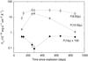 |
Fig. 5 Temporal evolution of the 10 μm continuum flux, the [Ni ii] 6.63 μm and the [Co ii] 10.52 μm line fluxes. |
3.4. The continuum emission at 10 μm
In Fig. 5 the evolution of the continuum flux at 10 μm is plotted with the [Co ii] 10.52μ and [Ni ii] 6.63μ line fluxes. There is a striking similarity between these curves and those of SN 1987A (cf. Fig. 2 in Roche et al. 1993). The evolution of the [Ni ii] and [Co ii] line fluxes were discussed above. The 10 μm flux values show a significant decline between +115 and 291 days, but after that they brighten up and by +510 days they reach the same level as in the earliest spectrum and only slightly decrease later.
Roche et al. (1993) explained the 10 μm light curve of SN 1987A as caused by optically thin free-free emission by ~300 days, then after ~500 days the increasing flux was interpreted as the sign of dust formation. We invoke the same mechanism for SN 2004dj to explain the 10 μm light curve here. Similar temporal evolution could be identified in the IRAC and MIPS light curves as well, which are discussed below.
3.5. Mid-IR light curves
 |
Fig. 6 IRAC (3.6 μm – open squares, 4.5 μm – filled squares, 5.8 μm – open circles, 8.0 μm – filled circles), IRS PUI (open triangles) and MIPS 24.0 μm (filled triangles) light curves of SN 2004dj. The excess emission appearing on 3.6, 5.8 and 8.0 μm peaks later at longer wavelengths, which is consistent with a warm, cooling dust formed one year after the core collapse. |
Similar to the temporal evolution of the 10 μm continuum flux (Fig. 5), the light curves of IRAC data from the 3.6 μm, 5.8 μm and 8.0 μm channels also show a significant peak after + 400 days post-explosion (Fig. 6). Such late-time MIR excess is usually considered as a strong evidence for the presence of dust. The excess emission peaks later at longer wavelengths, which is consistent with a model of warm, cooling dust grains formed in the ejecta. Unfortunately, there are no MIPS data during the peak of the IRAC light curves, but the 24 μm fluxes also show a slight excess after +800 days with respect to those obtained between +100−300 days.
The 4.5 μm fluxes do not show the peak that the other IRAC channels do. The most plausible explanation for this is the presence of the 1−0 vibrational band of CO at 4.65 μm (Sect. 3.2) that contributes significantly to the measured flux in the 4.5 μm channel. After ~+500 days when the CO band disappeared (Fig. 2), the light curve in this channel behaves similarly to those in the other IRAC bands.
In Fig. 7 the evolution of the MIR SED of SN 2004dj is plotted (a vertical shift has been applied between the data for better visibility). This figure further illustrates the disappearance of the CO band as well as the shifting of the peak of the SED toward longer wavelengths. The fitting of SEDs with dust models is presented in Sect. 4.
We conclude that the MIR excess flux present in all IRAC bands and also at longer wavelengths between ~+450−900 days is most likely caused by thermal emission of dust particles inside the SN ejecta. The significant increase and subsequent decrease of the excess emission on a timescale of a few hundred days argues against an IR-echo of the SN radiation from pre-existing CSM or ISM, because in that case the temporal evolution of the light curve should be at least one order of magnitude slower.
3.6. Polarization data
 |
Fig. 7 Evolution of MIR SEDs of SN 2004dj. |
 |
Fig. 8 Evolution of the detected true degree-of-polarization in SN 2004dj. Open symbols: spectropolarimetry by Leonard et al. (2006); filled symbol: imaging polarimetry with HST/ACS (this paper). |
The measured true degree-of-polarization ptrue = 0.81 ± 0.4% derived in Sect. 2.3 suggests a 2-sigma (weak) detection of polarized light from SN 2004dj in the optical (close to B-band) at +425 days. This phase is not covered well by the Spitzer observations, but it is at the beginning of the “MIR bump”-phase, when the suspected dust formation just started. The detected polarization, if real, fits nicely into this picture, as the photons scattered off the dust grains are expected to be polarized.
The source of the detected polarization may be interstellar, not related to the SN ejecta. To prove or reject this hypothesis, we used the spectropolarimetric results by Leonard et al. (2006). They detected changing net continuum polarization of SN 2004dj during early phases, starting close to zero, then climbing up to p = 0.55% at +90 days then declining as ~1/t2 to 0.052% by +270 days after explosion (see Fig. 8). On the other hand, the measured polarization in the optical spectral lines was much less, going below 0.1% in strong lines (Hα or the CaII triplet) and in the metallic line blends shortward of 5500 Å.
Leonard et al. (2006) also measured the interstellar polarization in the direction of SN 2004dj, and found pISM = 0.29%. Obviously our detection from HST at +425 days is significantly higher than pISM found by Leonard et al. Subtracting pISM ~ 0.3% from the total measured polarization, pSN ~ 0.5% remains, which is similar to the amount of net continuum polarization detected by Leonard et al. (2006) during the photospheric phase.
It must be emphasized that the source of the polarization during the photospheric phase (measured by Leonard et al. 2006) and the nebular phase presented here is very different. During the photospheric phase, the polarization is caused by Thompson-scattering, and the detected net polarization suggests an asymmetric shape of the inner ejecta (Leonard et al. 2006; Wang & Wheeler 2008). Leonard et al. also pointed out that this kind of polarization is expected to quickly decrease with time when the ejecta dilutes and the scattering optical depth declines, and this is exactly what they have observed (cf. Fig. 8). On the other hand, the polarization detected with HST at +425 days, when the ejecta are thought to be almost fully transparent and the electron scattering optical depth is much smaller, should be produced by scattering on other particles. Newly formed dust seems to be a plausible explanation, although some kind of deviation from spherical symmetry is still necessary to produce observable net polarization. One possibility may be the formation of dust clumps distributed asymmetrically in the SN ejecta. This was also proposed by e.g. Tran et al. (1997) to explain the observed polarization in SN 1993J. We conclude that the detected polarization, pSN ~ 0.5% at +425 days is likely caused by scattering on freshly formed dust particles, which agrees with other signs of dust formation after this epoch.
4. Models for dust
In the previous section we presented several pieces of evidence for the presence of dust around SN 2004dj. In order to analyze the physical properties and estimate the total amount of dust, we fit theoretical SEDs from analytic and numerical models to the measured IRAC and MIPS data (days 267−275, 849−883, 1006−1016 and 1236−1246, respectively). First, we use the analytic model described by Meikle et al. (2007), then we apply the numerical radiative-transfer code MOCASSIN (Ercolano et al. 2003, 2005). Prior to fitting, the observed SED fluxes were dereddened using the galactic reddening law parametrized by Fitzpatrick & Massa (2007) assuming RV = 3.1 and adopting E(B − V) = 0.1 from Paper I. The IRAC data were also corrected for the fluxes of the surrounding cluster as explained in Sect. 3.1. We assumed a general 10% uncertainty for all observed fluxes to represent the overall random plus systematic errors (see e.g. Kotak et al. 2005).
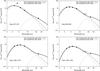 |
Fig. 9 Single-component blackbodies (optically thick case, dotted lines) and two-component analytic dust models (optically thin case, solid lines) compared to the MIR SEDs. At the first epoch, we eliminated the 4.5 μm point from the fitting, because of the excess flux from the 1 − 0 vibrational band of CO (see text for details). The IRS PUI fluxes are also shown as empty circles for illustration, but those were not included in the fitting. |
4.1. Analytic models
We fitted simple analytic models to the observed MIR SEDs using Eq. (1) in Meikle et al. (2007) assuming a homogeneous (constant-density) dust distribution. To estimate the dust optical depth (τλ), we adopted the power-law grain size distribution of Mathis et al. (1977, hereafter MRN) assuming m = 3.5 for the power-law index and amin = 0.005 μm and amax = 0.05 μm for the minimum and maximum grain sizes, respectively.
As there is no detectable 9.7 micron silicate feature in any of the observed SEDs, our initial fits using C-Si-PAH dust composition (Weingartner & Draine 2001) failed. The lack of detectable SiO emission in the IRS spectra (Fig. 2) also supports the absence of silicates in the dust composition.
Thus, we chose amorphous carbon (AC) grains for subsequent models. Values for the dust opacity κλ were taken from Colangeli et al. (1995). For the grain density we adopted ρgr = 1.85 g cm-3 as the value for the AC1 material given by Rouleau & Martin (1991; see e.g. Kotak et al. 2009; Botticella et al. 2009). The grain temperature T and the grain number density scaling factor (k) were free parameters during the fitting. The dust is assumed to be distributed uniformly within a sphere, the radius R of which was chosen using the maximum velocity of the SN ejecta during the nebular phase (vmax ~ 3250 km s-1, Paper II; see the method in Meikle et al. 2007), and assuming homologous expansion, i.e. R = vmax·t where t is the phase of the SN at the moment of the SED observation.
For SN 1987A Wooden et al. (1993) showed that a hot component (T ~ 5000 K, probably caused by an optically thick gas within the ejecta) affects the dust-emission continuum. On the other hand, Meikle et al. (2007) and Kotak et al. (2009) found that the contribution of the hot component is very small at wavelengths longer than 3 μm for SNe 2003gd and 2004et (also type II-P events). In a T = 6000 K, vhot = 60 km s-1 blackbody at +267 days (Kotak et al. 2009) this contribution is less than 1%. Late-time optical photometry of SN 2004dj was dominated by the flux from the cluster Sandage-96, which prevented the inclusion of optical measurements in the fitted SEDs. For these reasons, we neglected the presence of the hot component in the models.
Parameters for the best-fit analytic models to SN 2004dj SEDs.
Parameters for best-fit homogeneous MOCASSIN models to SN 2004dj SEDs.
The parameters of the best-fitting models are collected in Table 6. The radius of the dust-forming zone containing the newly formed warm dust, Rwarm, increased from 0.75 to 3.88 × 1016 cm between 270 and 1240 days, while during the same time its temperature decreased from 710 to 424 K. The flux from the cold component can be described by a simple blackbody with Tcold = 186−103 K and Rcold = 1.5−6.2 × 1016 cm.
The cumulative mass of freshly formed dust was calculated as Md = 4πR2τν/3κν (Lucy et al. 1989; Meikle et al. 2007) for each fitted epoch. The resulting masses are between 3.1 × 10⁻⁶ and 1.4 × 10⁻⁵ M⊙, but it should be noted that these masses from analytic models are actually lower limits (Meikle et al. 2007), because of the implicit assumption that the dust cloud has the lowest possible optical depth. Theoretical studies by Kozasa et al. (2009) also suggested that assuming optically thin dust opacity in the MIR leads to an underestimation of the total dust mass. More realistic dust masses can be obtained only from numerical models for the optically thick dust cloud (see below).
The last three columns in Table 6 contain the blackbody MIR luminosities, Lwarm and Lcold, calculated from the radii and temperatures of the warm and cold components, respectively. For comparison, the luminosity from the radioactive 56Co-decay (LCo) is also given, assuming 0.02 M⊙ for the initial Ni-mass (Paper I). Apparently the warm component dominates the MIR luminosity, which is comparable to LCo at ~270 days, but becomes orders of magnitude higher than LCo by ~850 days.
4.2. Numerical models
To model the optically-thick dust cloud around SN 2004dj, we applied the three-dimensional Monte Carlo radiative-transfer code MOCASSIN. This code was originally developed for modeling the physical conditions in photoionized regions (Ercolano et al. 2003, 2005). The code uses a ray-tracing technique, following the paths of photons emitted from a given source through a spherical shell containing a specified medium. For numerical calculations, the shell is mapped onto a Cartesian grid allowing light-matter interactions (absorption, re-emission and scattering events) and to track energy packets until they leave the shell and contribute to the observed SED. In newer versions it is possible to model environments that contain not only gas but also dust, or to assume pure dust regions (Ercolano et al. 2005, 2007). This can be applied to reconstruct dust-enriched environments of CC SNe and to determine physical parameters of the circumstellar medium (grain-size distribution, composition and geometry), as was shown by Sugerman et al. (2006) and Ercolano et al. (2007).
We used version 2.02.55 of MOCASSIN for the present study. We chose amorphous carbon for grain composition (optical constants were taken from Hanner 1988) for the same reason as during the fitting of analytic models described above. The original grid in the code allowed us to model uniform spatial distribution of grains. Thus, we first created constant-density dust shells.
We adopted four different grain-size distributions: MRN (with the same parameters as before) and three other cases of single-sized grains with radii of 0.005, 0.05 and 0.1 μm. With only small (r = 0.005 μm) grains, we could not reproduce the observed SEDs, but we found an adequate fitting for the other three cases. It agrees well with the calculations of Kozasa et al. (2009) that dust mass is dominated by grains with radii larger than 0.03 μm in type II-P SNe.
The final results of these calculations are shown in Table 7. For the best-fitting models, the illuminating source was given as a blackbody with TBB = 7000 K and L∗ = 2.2−4.5 × 10⁵ L⊙. The geometry of the dust cloud was assumed as a spherical shell with inner and outer radii Rin and Rout. For Rout we adopted the radius of the warm component (Rwarm) from the analytic models (corresponding to v ~ 3250 km s-1 in velocity space). The inner radius Rin was a free parameter, and the values that produced the best fit are shown in Table 7.
For the dust masses we obtained values between 2 − 8 × 10⁻⁴ M⊙, depending on the size and thickness of the dust cloud, which are more than one order of magnitude higher than the masses from analytic models. It should be noted, however, that in order to get satisfactory fitting of the MIPS fluxes, a cold blackbody component was added to the model with the same parameters as described in Sect. 4.1.
As a second step, we kept the MRN distribution, but generated shells with ρ ∝ r − n density profiles. We chose n = 7 because this density distribution was found when modeling the optical spectra of SN 2004dj during the photospheric phase (Paper I). These steep density distributions in the SN ejecta are also predicted by numerical simulations (e.g. Chugai et al. 2007; Utrobin 2007). We computed symmetric grids for the density distribution with 10 grid points on each axis, but for comparison we also produced models with higher resolution grids using 15, 30 and 49 grid points. These models were applied for the SED observed between 849-883 days (see the different models in Fig. 10). The previous values for Rout were again used.
Parameters for MOCASSIN models with power-law density distribution.
We show in Table 8 that the models with a power-law grain-density distribution led to somewhat different solutions, which resulted in dust masses one order of magnitude lower than in the case of constant-density models (but still 3 − 4 times higher than the results from analytic models). In order to test the effect of choosing n = 7 on the derived dust masses, we also generated a model assuming ρ ∝ r-2 density profile (e.g. Ercolano et al. 2007; Wesson et al. 2010). This density distribution is expected in a CSM produced by a stellar wind with constant outflow velocity. The resulting dust mass turned out to be a factor of 2 higher than in the case of n = 7 (see Table 8), but lower than the results from the constant-density models (Table 7).
 |
Fig. 10 Comparison of the best fitting analytic and MOCASSIN models with the observed SED for 849 − 883 days. See text and Tables 6 − 8 for the explanation of the different models. Models assuming the MRN grain-size distribution were found to be the best to reproduce the observations. The IRS PUI flux (empty circle) was not used during the fitting. |
4.3. Discussion of the dust models
The results of analytic and numerical modeling presented above confirm that the MIR SEDs can be well explained by assuming newly-formed dust in the ejecta of SN 2004dj. The lack of the observed spectral features of SiO and tests of different models yield amorphous carbon as the most likely grain composition. The best-fitting models give large (a ~ 0.05−0.1 μm) grains, which is consistent with recent theoretical studies of dust in type II-P SNe. Between +267 and +1246 days, the dust temperature decreased from ~700 to ~400 K. The lower limit for dust mass is 1.4 × 10⁻⁵ M⊙, while the highest mass derived from our models is 7.6 × 10⁻⁴ M⊙. The estimated amount of new dust around SN 2004dj is similar to those obtained for other type II SNe, and therefore does not prove that CC SNe are significant dust sources in the Universe.
Note that if the dust had been assumed to form optically-thick clumps (Lucy et al. 1989), the resulting dust mass would have been somewhat higher. Because the mass hidden by clumping depends on the actual number and optical depth of individual clumps, it is difficult to predict the dust mass unambiguously in such a model. Numerical simulations by Sugerman et al. (2006) and Ercolano et al. (2007) showed that the mass of hidden dust could be one order of magnitude higher than calculated with smooth density distribution. We did not investigate these models in detail, but mention that even if the dust distribution were clumpy around SN 2004dj, and the dust mass were one order of magnitude higher than estimated above, it still would not reach 0.01 M⊙.
The modeling of the SEDs revealed a cold component as a T ~ 110 K temperature shell lying at 1.5 − 6 × 1016 cm away from the central source. The location of this component is in the outer region (v ~ 6400 km s-1) of the SN ejecta, where the ejecta/CSM interaction is expected to take place. Such a cold component with similar temperature (T ~ 100 K) was found in SN 2004et by Kotak et al. (2009), and also in SN 2002hh, although the latter is slightly warmer (T ~ 300 K, Meikle et al. 2006). However, the cold components in these type II-P SNe were attributed to an IR-echo, i.e. a radiation from pre-existing dust reheated by the strong UV/optical radiation from the SN close to maximum light.
 |
Fig. 11 Geometrical model of warm (inner, gray) and cold (outer, hatched) dust shells around SN 2004dj at ~850 days |
Although pre-existing dust around SN 2004dj seems to be a plausible explanation for the early radio/X-ray detection (Chevalier et al. 2006), we do not favor the IR-echo hypothesis as the cause of the MIR cold component in this case. There are several arguments that do not support the probability of the IR-echo. First, both SNe 2002hh and 2004et were moderately or highly reddened (AV > 1 mag), while the reddening of SN 2004dj was much less (AV ≤ 0.3 mag, Paper I). Thus, pre-existing CSM dust, if present, should have been much less dense around 2004dj than in 2002hh or 2004et. Second, the surrounding cluster, S96, is a young (t ~ 10 Myr), very compact cluster with a significant OB-star population (Maiz-Apellaniz et al. 2004, Paper II). Strong UV/optical radiation from nearby OB-stars should expel the ISM/dust from the cluster, although some CSM around massive stars resulting from mass loss via stellar wind might still be present. Third, the early UV/X-ray flash of the SN should create a dust-free cavity within a region of ~1016−1017 cm in size after core collapse and around maximum light (Dwek 1983, 1985). The radii of the dust models that fit the observed MIR SEDs are within this region, therefore the MIR radiation should come mostly from inside the cavity. Pre-existing dust within this region is unlikely. We also emphasize that the dust cloud around SN 2004et was found to have a roughly constant size (Kotak et al. 2009), while our models for SN 2004dj clearly indicate that the dust regions expand homologuously with the ejecta. For these reasons, we do not expect that either the cold or the warm component is caused by IR-echo, although some pre-existing CSM at higher distance cannot be ruled out completely.
Another more probable possibility for the cold component is the condensation of dust grains in a CDS between the forward and reverse shocks (Sect. 1). Although this mechanism is supposed to work predominantly in type IIn SNe because of the higher density CSM, there are hints of a similar process taking place around SN 2004dj. Chevalier et al. (2006) pointed out based on radio and X-ray observations of Beswick et al. (2005) and Pooley & Lewin (2004) that there is a non-negligible amount of CSM around SN 2004dj, probably produced by stellar wind from the progenitor, which has an estimated mass-loss rate of ~10-6 M⊙ yr-1. Chugai et al. (2007) presented similar results from studying the observed Hα profiles during the photospheric and early nebular phase. They argued that the observed high-velocity absorption “notch” features could not form in the unshocked ejecta, instead, they are supposed to be produced by the CDS modified by Rayleigh-Taylor instability. Applying Eq. (10) of Chugai et al. (2007), the expected radius of the continously growing CDS is 1.9−7.0 × 1016 cm between +267 and +1246 days in a self-similar model. These values agree well with the size of the cold component involved in our models (see Table 6), which strengthens the assumption that CDS plays a role in producing the MIR SEDs.
5. Summary
Using public data of Spitzer- and Hubble space telescope, we presented a detailed analysis of MIR light curves and spectra on SN 2004dj between +98 and +1381 days after explosion. Following SN 2004et (Kotak et al. 2009), this is the second long-term study of the dust-formation processes around a type II-P supernova. We found several pieces of evidence for dust formation after explosion. These include
-
significant brightening in MIR light curves starting after +400 days;
-
detection of ~0.5% polarization from the SN ejecta in the optical (HST F435W filter) at +425 days.
Acknowledgments
We would like to thank the referee J. Danziger for the critical but very useful comments, which helped us to improve the paper. Thanks are also due to P. Meikle for his valuable comments and suggestions on the dust models, B. Ercolano for sending us her MOCASSIN code ver. 2.02.55 and for her extensive help in running the code, and L. Colangeli and V. Mennella for providing the electronic version of their table about mass-extinction coefficients of carbon grains. Fruitful discussions with N. Chugai, J. C. Wheeler, and S. D. Van Dyk are gratefully acknowledged. This work is based on observations made with the Spitzer space telescope, which is operated by the Jet Propulsion Laboratory, California Institute of Technology under a contract with NASA. Some of the data presented in this paper were obtained from the Multimission Archive at the Space Telescope Science Institute (MAST). STScI is operated by the Association of Universities for Research in Astronomy, Inc., under NASA contract NAS5-26555. Support for MAST for non-HST data is provided by the NASA Office of Space Science via grant NNX09AF08G and by other grants and contracts. This work is supported by the Hungarian OTKA Grants K76816 and MB08C 81013, the University of Sydney, NSF Grant AST-0707669, the Texas Advanced Research Program grant ASTRO-ARP-0094 and the “Lendület” Young Researchers’ Program of the Hungarian Academy of Sciences.
References
- Andrews, J. E., Gallagher, J. S., Clayton, G. C., et al. 2010, ApJ, 715, 541 [NASA ADS] [CrossRef] [Google Scholar]
- Barlow, M. J., Sugerman, B. E. K., Fabbri, J., et al. 2005, ApJ, 627, L113 [NASA ADS] [CrossRef] [Google Scholar]
- Bertoldi, F., Carilli, C. L., Cox, P., et al. 2003, A&A, 406, L55 [NASA ADS] [CrossRef] [EDP Sciences] [Google Scholar]
- Beswick, R. J., Muxlow, T. W. B., Argo, M. K., et al. 2005, ApJ, 623, L21 [NASA ADS] [CrossRef] [Google Scholar]
- Bianchi, S., & Schneider, R. 2007, MNRAS, 378, 973 [NASA ADS] [CrossRef] [Google Scholar]
- Biretta, J., Kozhurina-Platais, V., Boffi, F., Sparks, W., & Walsh, J. 2004, STScI Instr. Sci. Rep. ACS 2004-09 [Google Scholar]
- Blair, W. P., Ghavamian, P., Long, K. S., et al. 2007, ApJ, 662, 998 [NASA ADS] [CrossRef] [Google Scholar]
- Bode, M. F., & Evans, A. 1980, MNRAS, 193, 21 [NASA ADS] [Google Scholar]
- Botticella, M. T., Pastorello, A., Smartt, S. J., et al. 2009, MNRAS, 398, 1041 [NASA ADS] [CrossRef] [Google Scholar]
- Cernuschi, F., Marsicano, F. R., & Codina, S. 1967, Ann. d’Astrophys., 30, 1039 [Google Scholar]
- Chevalier, R. A. 1982, ApJ, 258, 790 [Google Scholar]
- Chevalier, R. A., Fransson, C., & Nymark, T. K. 2006, ApJ, 641, 1029 [NASA ADS] [CrossRef] [Google Scholar]
- Chieffi, A., & Limongi, M. 2004, ApJ, 608, 405 [NASA ADS] [CrossRef] [Google Scholar]
- Chugai, N. N., Chevalier, R. A., & Utrobin, V. P. 2007, ApJ, 662, 1136 [NASA ADS] [CrossRef] [EDP Sciences] [Google Scholar]
- Clayton, D. D. 1979, Ap&SS, 65, 179 [NASA ADS] [CrossRef] [Google Scholar]
- Clayton, D. D., & Nittler, L. R. 2004, ARA&A, 42, 39 [NASA ADS] [CrossRef] [Google Scholar]
- Clayton, D. D., Amari, S., & Zinner, E. 1997, Ap&SS, 251, 355 [NASA ADS] [CrossRef] [Google Scholar]
- Colangeli, L., Mennella, V., Palumbo, P., Rotundi, A., & Bussoletti, E. 1995, A&AS, 113, 561 [Google Scholar]
- Danziger, I. J., Gouiffes, C., Bouchet, P., & Lucy, L. B. 1989, IAU Circ., 4746 [Google Scholar]
- Danziger, I. J., Lucy, L. B., Bouchet, P., & Gouiffes, C. 1991, in The Tenth Santa Cruz Workshop in Astronomy and Astrophysics, ed. S. E. Woosley (New York: Springer-Verlag), 69 [Google Scholar]
- Dolphin, A. E. 2000, PASP, 112, 1383 [NASA ADS] [CrossRef] [Google Scholar]
- Dunne, L., Eales, S., Ivison, R., Morgan, H. L., & Edmunds, M. G. 2003, Nature, 424, 285 [NASA ADS] [CrossRef] [PubMed] [Google Scholar]
- Draine, B. T. 2003, ARA&A, 41, 241 [NASA ADS] [CrossRef] [Google Scholar]
- Draine, B. T. 2009, in Cosmic Dust – Near and Far, ed. T. Henning, E. Grün, & J. Steinacker (San Francisco: ASP), ASP Conf. Ser., 414, 453 [Google Scholar]
- Dwek, E. 1983, ApJ, 274, 175 [NASA ADS] [CrossRef] [Google Scholar]
- Dwek, E. 1985, ApJ, 297, 719 [NASA ADS] [CrossRef] [Google Scholar]
- Dwek, E., Galliano, F., & Jones, A. P. 2007, ApJ, 662, 927 [NASA ADS] [CrossRef] [Google Scholar]
- Elmhamdi, A., Danziger, I. J., Chugai, N., et al. 2003, MNRAS, 338, 939 [NASA ADS] [CrossRef] [Google Scholar]
- Elmhamdi, A., Danziger, I. J., Cappellaro, E., et al. 2004, A&A, 426, 963 [NASA ADS] [CrossRef] [EDP Sciences] [Google Scholar]
- Elvis, M., Marengo, M., & Karovska, M. 2002, ApJ, 567, L107 [NASA ADS] [CrossRef] [Google Scholar]
- Engelbracht, C. W., Blaylock, M., Su, K. Y. L., et al. 2007, PASP, 119, 994 [NASA ADS] [CrossRef] [Google Scholar]
- Ercolano, B., Barlow, M. J., Storey, P. J., & Liu, X.-W. 2003, MNRAS, 340, 1153 [NASA ADS] [CrossRef] [Google Scholar]
- Ercolano, B., Barlow, M. J., & Storey, P. J. 2005, MNRAS, 362, 1038 [NASA ADS] [CrossRef] [Google Scholar]
- Ercolano, B., Barlow, M. J., & Sugerman, B. E. K. 2007, MNRAS, 375, 753 [NASA ADS] [CrossRef] [Google Scholar]
- Fitzpatrick, E. L., & Massa, D. 2007, ApJ, 663, 320 [NASA ADS] [CrossRef] [EDP Sciences] [Google Scholar]
- Fox, O., Skrutskie, M. F., Chevalier, R. A., et al. 2009, ApJ, 691, 650 [NASA ADS] [CrossRef] [Google Scholar]
- Gerardy, C. L., Fesen, R. A., Nomoto, K., et al. 2002, ApJ, 575, 1007 [NASA ADS] [CrossRef] [Google Scholar]
- Hanner, M. S. 1988, NASA Conf. Publ., 3004, 22 [Google Scholar]
- Hoyle, F., & Wickramasinghe, N. C. 1970, Nature, 226, 2 [Google Scholar]
- Kotak, R., Meikle, W. P. S., van Dyk, S. D., Höflich, P. A., & Mattila, S. 2005, ApJ, 628, L123 [NASA ADS] [CrossRef] [Google Scholar]
- Kotak, R., Meikle, P., Pozzo, M., et al. 2006, ApJ, 651, L117 [NASA ADS] [CrossRef] [Google Scholar]
- Kotak, R., Meikle, W. P. S., Farrah, D., et al. 2009, ApJ, 704, 306 [NASA ADS] [CrossRef] [Google Scholar]
- Kozasa, T., Nozawa, T., Tominaga, N., et al. 2009, in Cosmic Dust – Near and Far, ed. T. Henning, E. Grün, & J. Steinacker (San Francisco: ASP), ASP Conf. Ser., 414, 43 [Google Scholar]
- Krause, O., Birkmann, S. M., Rieke, G. H., et al. 2004, Nature, 432, 596 [NASA ADS] [CrossRef] [PubMed] [Google Scholar]
- Leonard, D. C., Filippenko, A. V., Ganeshalingam, M., et al. 2006, Nature, 440, 505 [NASA ADS] [CrossRef] [PubMed] [Google Scholar]
- Lucy, L. B., Danziger, I. J., Gouiffes, C., & Bouchet, P. 1989, in Structure and Dynamics of the Interstellar Medium, ed. G. Tenorio-Tagle et al. (Berlin: Springer), 164 [Google Scholar]
- Lucy, L. B., Danziger, I. J., Gouiffes, C., & Bouchet, P. 1991, in The Tenth Santa Cruz Workshop in Astronomy and Astrophysics, ed. S. E. Woosley (New York: Springer-Verlag), 82 [Google Scholar]
- Maiolino, R., Schneider, R., Oliva, E., et al. 2004, Nature, 431, 533 [NASA ADS] [CrossRef] [PubMed] [Google Scholar]
- Maíz-Apellániz, J., Bond, H. E., Siegel, M. H., et al. 2004, ApJ, 615, L113 [NASA ADS] [CrossRef] [Google Scholar]
- Markwick-Kemper, F., Gallagher, S. C., Hines, D. C., & Bouwman, J. 2007, ApJ, 668, L107 [NASA ADS] [CrossRef] [Google Scholar]
- Mathis, J. S., Rumpl, W., & Nordsieck, K. H. 1977, ApJ, 217, 425 [NASA ADS] [CrossRef] [Google Scholar]
- Mattila, S., Meikle, W. P. S., Lundqvist, P., et al. 2008, MNRAS, 389, 141 [NASA ADS] [CrossRef] [Google Scholar]
- Matsuura, M., Barlow, M. J., Zijlstra, A. A., et al. 2009, MNRAS, 396, 918 [NASA ADS] [CrossRef] [Google Scholar]
- Meikle, W. P. S., Mattila, S., Gerardy, C. L., et al. 2006, ApJ, 649, 332 [NASA ADS] [CrossRef] [Google Scholar]
- Meikle, W. P. S., Mattila, S., Pastorello, A., et al. 2007, ApJ, 665, 608 [NASA ADS] [CrossRef] [Google Scholar]
- Michalowski, M. J., Watson, D., & Hjorth, J. 2010, ApJ, 712, 942 [NASA ADS] [CrossRef] [Google Scholar]
- Morgan, H. L., & Edmunds, M. G. 2003, MNRAS, 343, 427 [NASA ADS] [CrossRef] [EDP Sciences] [Google Scholar]
- Morgan, H. L., Dunne, L., Eales, S. A., Ivison, R. J., & Edmunds, M. G. 2003, ApJ, 597, L33 [NASA ADS] [CrossRef] [Google Scholar]
- Nakano, S., Itagaki, K., Bouma, R. J., Lehky, M., & Homoch, K. 2004, IAU Circ., 8377 [Google Scholar]
- Nomoto, K., Tominaga, N., Umeda, H., Kobayashi, C., & Maeda, K. 2006, Nuclear Physics A, 777, 424 [Google Scholar]
- Nozawa, T., Kozasa, T., Umeda, H., Maeda, K., & Nomoto, K. 2003, ApJ, 598, 785 [NASA ADS] [CrossRef] [Google Scholar]
- Nozawa, T., Kozasa, T., Tominaga, N., et al. 2008, ApJ, 684, 1343 [NASA ADS] [CrossRef] [Google Scholar]
- Patat, F., Benetti, S., Pastorello, A., & Filippenko, A. V. 2004, IAU Circ., 8378 [Google Scholar]
- Pei, Y. C., Fall, S. M., & Bechtold, J. 1991, ApJ, 378, 6 [NASA ADS] [CrossRef] [Google Scholar]
- Pettini, M., King, D. L., Smith, L. J., & Hunstead, R. W. 1997, ApJ, 478, 536 [NASA ADS] [CrossRef] [Google Scholar]
- Pooley, D., & Lewin, W. H. G. 2004, IAU Circ. 8390 [Google Scholar]
- Pozzo, M., Meikle, W. P. S., Fassia, A., et al. 2004, MNRAS, 352, 457 [NASA ADS] [CrossRef] [Google Scholar]
- Prieto, J. L., Kistler, M. D., Thompson, T., et al. 2008, ApJ, 681, L9 [NASA ADS] [CrossRef] [Google Scholar]
- Reach, W. T., et al. 2006, Infrared Array Camera Data Handbook, v. 3.0, Spitzer Science Center, California Institute of Technology [Google Scholar]
- Rho, J., Kozasa, T., Reach, W. T., et al. 2008, ApJ, 673, 271 [NASA ADS] [CrossRef] [Google Scholar]
- Roche, P. F., Aitken, D. K., & Smith, C. H. 1993, MNRAS, 261, 522 [NASA ADS] [Google Scholar]
- Rouleau, F., & Martin, P. G. 1991, ApJ, 377, 526 [NASA ADS] [CrossRef] [Google Scholar]
- Sakon, I., Onaka, T., Wada, T., et al. 2009, ApJ, 692, 546 [Google Scholar]
- Sandstrom, K. M., Bolatto, A. D., Stanimirovic, S., van Loon, J. T., & Smith, J. D. 2009, ApJ, 696, 2138 [NASA ADS] [CrossRef] [Google Scholar]
- Schuster, M. T., Marengo, M., & Patten, B. M. 2006, in Observatory Operations: Strategies, Processes, and Systems, ed. D. R. Silva, & R. E. Doxsey, Proc. SPIE, 6270, 627020 [Google Scholar]
- Silvia, D. W., Smith, B. D., & Shull, J. M. 2010, ApJ, 715, 1575 [NASA ADS] [CrossRef] [Google Scholar]
- Smith, N., Foley, R. J., & Filippenko, A. V. 2008a, ApJ, 680, 568 [NASA ADS] [CrossRef] [Google Scholar]
- Smith, N., Chornock, R., Li, W., et al. 2008b, ApJ, 686, 467 [NASA ADS] [CrossRef] [Google Scholar]
- Smith, N., Silverman, J. M., Chornock, R., et al. 2009, ApJ, 695, 1334 [NASA ADS] [CrossRef] [Google Scholar]
- Sparks, W. B., & Axon, D. J. 1999, PASP, 111, 1298 [Google Scholar]
- Stanimirovic, S., Bolatto, A. D., Sandstrom, K. M., et al. 2005, ApJ, 632, L103 [NASA ADS] [CrossRef] [Google Scholar]
- Stobie, E., & Ferro, A. 2006, in Astronomical Data Analysis Software and Systems XV, ed. C. Gabriel, C. Arviset, D. Ponz, & E. Solano, Proc. ASP Conf. Ser., 351, 540 [Google Scholar]
- Stratta, G., Maiolino, R., Fiore, F., & D’Elia, V. 2007, ApJ, 661, L9 [NASA ADS] [CrossRef] [Google Scholar]
- Sugerman, B. E. K. 2003, AJ, 126, 1939 [NASA ADS] [CrossRef] [Google Scholar]
- Sugerman, B. E. K., Ercolano, B., Barlow, M. J., et al. 2006, Science, 313, 196 [NASA ADS] [CrossRef] [PubMed] [Google Scholar]
- Thielemann, F.-K., Nomoto, K., & Hashimoto, M. 1996, ApJ, 460, 408 [NASA ADS] [CrossRef] [Google Scholar]
- Todini, P., & Ferrara, A. 2001, MNRAS, 325, 726 [NASA ADS] [CrossRef] [Google Scholar]
- Tominaga, N., Limongi, M., Suzuki, T., et al. 2008, ApJ, 687, 1208 [NASA ADS] [CrossRef] [Google Scholar]
- Tran, H. D., Filippenko, A. V., Schmidt, G. D., et al. 1997, PASP, 109, 489 [NASA ADS] [CrossRef] [Google Scholar]
- Utrobin, V. P. 2007, A&A, 461, 233 [NASA ADS] [CrossRef] [EDP Sciences] [Google Scholar]
- Valiante, R., Schneider, R., Bianchi, S., & Andersen, A. C. 2009, MNRAS, 397, 1661 [NASA ADS] [CrossRef] [Google Scholar]
- Vinkó, J., Takáts, K., Sárneczky, K., et al. 2006, MNRAS, 369, 1780 (Paper I) [NASA ADS] [CrossRef] [Google Scholar]
- Vinkó, J., Sárneczky, K., Balog, Z., et al. 2009, ApJ, 695, 619 (Paper II) [NASA ADS] [CrossRef] [Google Scholar]
- Wang, L., & Wheeler, J. C. 2008, ARA&A, 46, 433 [NASA ADS] [CrossRef] [Google Scholar]
- Wang, X., Yang, Y., Zhang, T., et al. 2005, ApJ, 626, L89 [NASA ADS] [CrossRef] [Google Scholar]
- Weingartner, J. C., & Draine, B. T. 2001, ApJ, 548, 296 [NASA ADS] [CrossRef] [Google Scholar]
- Wesson, R., Barlow, M. J., Ercolano, B., et al. 2010, MNRAS, 403, 474 [NASA ADS] [CrossRef] [Google Scholar]
- Wooden, D. H., Rank, D. M., Bregman, J. D., et al. 1993, ApJS, 88, 477 [NASA ADS] [CrossRef] [Google Scholar]
- Woosley, S. E., & Weaver, T. A. 1995, ApJS, 101, 181 [NASA ADS] [CrossRef] [Google Scholar]
- Woosley, S. E., Heger, A., & Weaver, T. A. 2002, Rev. Mod. Phys., 74, 1015 [NASA ADS] [CrossRef] [Google Scholar]
- Zafar, T., Watson, D. J., Malesani, D., et al. 2010, A&A, 515, 94 [Google Scholar]
All Tables
All Figures
|
Fig. 1 Post-BCD images showing the environment of SN 2004dj obtained with Spitzer on 2004-10-12: IRAC 3.6 micron (top left), 5.8 micron (top right), 8.0 micron (bottom left), and MIPS 24.0 micron (bottom right). The SN is marked in each panel. The target is very faint on the MIPS image, which illustrates the necessity of PSF-photometry (see text for details). |
| In the text | |
|
Fig. 2 IRS spectra of SN 2004dj in the nebular phase. Line identification is based on Kotak et al. (2005, 2006). The evolution of the features is discussed in Sect. 3.2. |
| In the text | |
|
Fig. 3 Best-fitting model SEDs for the host cluster Sandage-96 from Paper II. Filled circles represent observed data for the cluster, while open symbols denote the averaged MIR-fluxes from the models (see Table 4). |
| In the text | |
|
Fig. 4 Ni and Co masses in M⊙ calculated from the strength of forbidden emission lines via Eq. (3). Open symbols: Ni-masses from the [Ni ii] 6.63 μ feature; filled symbols: Co-masses from the [Co ii] 10.52 μ feature. Lines show the expected amount of Co predicted from the radioactive decay of 0.02 M⊙ radioactive 56Ni synthesized in the explosion. Continuous line: only 56Co; dashed line: 56Co plus 57Co with solar abundance ratio; dotted line: 56Co plus 57Co assuming twice solar abundance ratio. |
| In the text | |
|
Fig. 5 Temporal evolution of the 10 μm continuum flux, the [Ni ii] 6.63 μm and the [Co ii] 10.52 μm line fluxes. |
| In the text | |
|
Fig. 6 IRAC (3.6 μm – open squares, 4.5 μm – filled squares, 5.8 μm – open circles, 8.0 μm – filled circles), IRS PUI (open triangles) and MIPS 24.0 μm (filled triangles) light curves of SN 2004dj. The excess emission appearing on 3.6, 5.8 and 8.0 μm peaks later at longer wavelengths, which is consistent with a warm, cooling dust formed one year after the core collapse. |
| In the text | |
|
Fig. 7 Evolution of MIR SEDs of SN 2004dj. |
| In the text | |
|
Fig. 8 Evolution of the detected true degree-of-polarization in SN 2004dj. Open symbols: spectropolarimetry by Leonard et al. (2006); filled symbol: imaging polarimetry with HST/ACS (this paper). |
| In the text | |
|
Fig. 9 Single-component blackbodies (optically thick case, dotted lines) and two-component analytic dust models (optically thin case, solid lines) compared to the MIR SEDs. At the first epoch, we eliminated the 4.5 μm point from the fitting, because of the excess flux from the 1 − 0 vibrational band of CO (see text for details). The IRS PUI fluxes are also shown as empty circles for illustration, but those were not included in the fitting. |
| In the text | |
|
Fig. 10 Comparison of the best fitting analytic and MOCASSIN models with the observed SED for 849 − 883 days. See text and Tables 6 − 8 for the explanation of the different models. Models assuming the MRN grain-size distribution were found to be the best to reproduce the observations. The IRS PUI flux (empty circle) was not used during the fitting. |
| In the text | |
|
Fig. 11 Geometrical model of warm (inner, gray) and cold (outer, hatched) dust shells around SN 2004dj at ~850 days |
| In the text | |
Current usage metrics show cumulative count of Article Views (full-text article views including HTML views, PDF and ePub downloads, according to the available data) and Abstracts Views on Vision4Press platform.
Data correspond to usage on the plateform after 2015. The current usage metrics is available 48-96 hours after online publication and is updated daily on week days.
Initial download of the metrics may take a while.