| Issue |
A&A
Volume 527, March 2011
|
|
|---|---|---|
| Article Number | A125 | |
| Number of page(s) | 9 | |
| Section | Astrophysical processes | |
| DOI | https://doi.org/10.1051/0004-6361/201015619 | |
| Published online | 09 February 2011 | |
Isotropic ion distribution functions triggered by consecutive solar wind bulk velocity jumps: a new equilibrium state
Argelander Institut für Astronomie der Universität Bonn,
Abteilung f. Astrophysik und Extraterrestrische
Forschung, Auf dem Huegel 71,
53121
Bonn,
Germany
e-mail: This email address is being protected from spambots. You need JavaScript enabled to view it.
Received:
20
August
2010
Accepted:
9
December
2010
Abstract
Context. Throughout the heliosphere, ion power spectra have been found in observations to exhibit suprathermal tails that follow power laws. Ion power-law spectra, though having a broad range of spectral indices 4.4 ≤ γv ≤ 6.6, perhaps favourably seem to have velocity power indices of γv ≃ (−5), a phenomenon that can more or less ubiquitously be found in heliospheric space plasmas. This is probably indicative of an as yet unidentified quasi-equilibrium state of collisionless space plasmas.
Aims. We develop the idea that these forms of ion spectra could be produced by a continuous back- and forth- shuffling of wind convected ions in consecutive jumps from fast to slow, and vice-versa, bulk velocity regimes.
Methods. The appearance of a quasi-equilibrium state due to this shuffling and re-shuffling, as we show, naturally results in ion distribution functions that are superpositions of a series of weighted Maxwellians resulting into power laws beyond a critical velocity border. Spectral intensities thereby anticorrelate with bulk velocities, but power indices depend only slightly on bulk velocity.
Results. The fully developed equilibrium state is shown here, however, to be characterized by a power law with power index γv = ( − 3), instead of 4.4 ≤ γv ≤ 6.6. These latter states, which generally show up in observations, thus may characterize an off-equilibrium state as we discuss in this paper.
Key words: shock waves / plasmas / magnetohydrodynamics (MHD) / solar wind
© ESO, 2011
1. Introduction
Many observers have obtained comprehensive in-situ spacecraft data of ion distribution functions in near and far interplanetary space, almost consistently confirming that interplanetary ion energy distribution functions in specific energy ranges clearly follow power-law distributions. The relation between differential flux j(E) and distribution function f(E) is given in the form j(E) = 2Ef(E)/m2, where E and m are the energy and mass of the ion, which makes it clearly evident that a power-law distribution of f(v) ~ v − κv (after applying the relation E = mv2/2) is identical to a differential flux function j(E) ~ E − κE ~ E − (κv/2 − 1). An interesting discovery by VOYAGER-1/-2 (Decker et al. 2005, 2008) was that in both the supersonic solar wind regime upstream from the termination shock and the subsonic regime downstream, differential intensities were fairly consistent with an energy power index of κE ≃ 1.5 yielding a velocity power index of κv = 5. Although this index κv = 5 has often been confirmed for ion distributions in the inner heliosphere (Gloeckler 2003; Fisk & Gloeckler 2006, 2008; Dayeh et al. 2009a,b), there is still doubt as to whether it can be called an ubiquitously valid power index, since many deviations from that index have been found, especially for ions heavier than protons.
Hill et al. (2009) found for He+ ions steeper spectra with κv ≥ 5. Dayeh et al. (2009b) studied heavy ion distributions (e.g. C, O, Fe) in interplanetary space at energies between 0.04 and 2.56 MeV/nucleon and found suprathermal tails with spectral indices κE between 1.27 and 2.29, corresponding to velocity indices of 4.5 ≤ κv ≤ 6.6 with a tendency for heavier ion suprathermal tails to be harder than lighter ion tails. This leads to the puzzling observational situation that though suprathermal ion tails often show power laws with κv ≃ 5, they also often exhibit significant deviations from that index. Theoreticians searching for explanations of these fairly unclear observational situations thus have to very carefully study conditions under which these ion spectral features have been observed.
Extended tails of ion distribution functions are most often ascribed to the interaction of these ions with different forms of compressive plasma turbulence connected with fluctuations δU in the local bulk velocity U of the background wind. This phenomenon was originally described as transit-time damping (see Fisk 1976; Toptygin 1983; Fichtner et al. 1996; le Roux & Fichtner 1999; Chalov et al. 1997; Chalov 2005).
Fisk & Gloeckler (2006, 2007, 2008) attempted to describe the appearance of energetic ion tails with the help of the phase-space transport equation derived by Parker (1965) as a stationary quasi-equilibrium state of a plasma interacting with compressive turbulence in thermally isolated systems. They consider how stochastic fluctuations of the bulk velocity of the background plasma lead to a well-tuned energy diffusion effect composed of adiabatic pumping in the core and spatial diffusion leaving through the tail. However, since in their approaches, the correct choice of system boundary conditions and construction of ensemble averages, as a statistical representation of different realisations of ion distribution functions, is contraversial (see Jokipii & Lee 2010), we present in this paper an independent, perhaps complementary study of the effect of bulk velocity fluctuations on the shape of ion distribution functions.
To study the phase-space behaviour of ions at their re-integration from one wind frame with
velocity U into another frame with U∗, it is
helpful to use some auxiliary physical quantities such as phase-space particle invariants.
From basic plasma physics, It is well known that in the absence of stochastic processes,
such as collisions or wave-particle interactions ions moving along magnetic fields with a
non-zero field-magnitude gradient along the field line, behave such that they conserve a
dynamic quantity called their magnetic moment  (see e.g.
Treumann & Baumjohann 1997). Furthermore,
we note that this quantity Γ also plays the role of an invariant under conditions when ions
are co-convected with a plasma bulk containing a frozen-in magnetic field, a typical
condition for ions convected by the solar wind.
(see e.g.
Treumann & Baumjohann 1997). Furthermore,
we note that this quantity Γ also plays the role of an invariant under conditions when ions
are co-convected with a plasma bulk containing a frozen-in magnetic field, a typical
condition for ions convected by the solar wind.
In the direction of the bulk flow, if the frozen-in magnetic field magnitude decreases, as for the Archimedian spiral field in the inner heliosphere (see Parker 1958; Forsyth et al. 2002), then it can be shown that bulk-convected ions conserve their magnetic moment Γ (see Fahr 2007; Fahr & Siewert 2008; Fahr & Siewert 2010b). The only restriction hereby is that typical periods τB of the field magnitude changes are large compared to the ion gyroperiods τg, which guarantees that an adiabatic adaptation to changes in the field magnitude by the gyrating ions can occur.
In addition, the differential motions of ions parallel to frozen-in fields, for bulk velocity gradients parallel to the field, exhibit a quantity that can serve as a second particle invariant Γ∥ = v∥B/ρ (Fahr & Siewert 2008; Siewert & Fahr 2008) closely related to the well-known second plasma invariant in the CGL-theory ΓCGL,2 = P∥B2/ρ3 (Chew et al. 1956).
These ion invariants cannot only profitably be used to describe the change in the dynamical
properties of ions at their passage during the solar wind termination shock (see Fahr & Siewert 2008, 2009; Fahr & Siewert
2010b), but are also applicable to any travelling bulk velocity jumps, when transit
times τt = ΔL/ΔU are much
shorter than spatial diffusion times  (see Toptygin 1983; Chalov et al. 1997).
Hereby ΔL is the extent of the transition region from one to the other bulk
velocity, i.e. from U1 to U2,
ΔU = U1 − U2
denotes the bulk velocity jump, LU is the scale
of a mono-bulk domain, v is the ion velocity, and Λ is the ion mean free
path with respect to wave scattering.
(see Toptygin 1983; Chalov et al. 1997).
Hereby ΔL is the extent of the transition region from one to the other bulk
velocity, i.e. from U1 to U2,
ΔU = U1 − U2
denotes the bulk velocity jump, LU is the scale
of a mono-bulk domain, v is the ion velocity, and Λ is the ion mean free
path with respect to wave scattering.
At a standing shock an abrupt decrease in the solar wind bulk velocity connected to an increase in the ion densities and frozen-in magnetic field magnitudes occurs. The description turns out to be fairly similar for the change in ion distribution functions at travelling bulk velocity jumps wherever they may occur. We now study this context further down in this paper.
2. Theoretical treatment of stationary shocks
We begin with the requirements motivated above and quantitatively formulated in Siewert & Fahr (2008). When applied to two
adjacent regions 1 and 2 of different bulk velocities U1 and
U2, one can identify two possibly conserved properties. First,
there is the classical electrodynamic invariant, the magnetic moment,  (1)and second,
there is the differential bulk drift
(1)and second,
there is the differential bulk drift 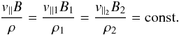 (2)These invariants
can be considered valid as long as diffusion times are much longer than transit times, i.e.
(2)These invariants
can be considered valid as long as diffusion times are much longer than transit times, i.e.
 . Therefore, this condition may
become invalid for large ion velocities with
. Therefore, this condition may
become invalid for large ion velocities with  , perhaps restricting the validity
of the following derivations of this paper to ions with sub-critical velocities
v ≤ vc. We study this in more detail later in
the paper.
, perhaps restricting the validity
of the following derivations of this paper to ions with sub-critical velocities
v ≤ vc. We study this in more detail later in
the paper.
2.1. Individual particle velocites at a stationary shock
We first study a general standing shock-like MHD feature with a surface normal
n pointing antiparallel to the solar wind flow vector
U, i.e. antiradial, while the wind flows in the radial
direction. Introducing the angle
θ = ∠(n,U),
this corresponds to θ = 180°. From existing solar wind data taken at
varying solar wind bulk velocities, it follows that mass flow continuity is fulfilled
essentially in the form of a causally connected one-dimensional flow without sources (see
McComas et al. 2000, 2003; Richardson et al. 2003),
which may be described by the following relation at larger solar distances
 (3)i.e. the solar wind
behaves as a source-free connection of flows fulfilling mass-flow conservation. Here the
parameters U1,2 denote fast and slow bulk velocities upstream
and downstream of an MHD shock with θ = 180°, or, more generally, the
normal bulk velocity components upstream and downstream in the case of
0° < θ < 180°, which is given e.g., at the solar wind
termination shock.
(3)i.e. the solar wind
behaves as a source-free connection of flows fulfilling mass-flow conservation. Here the
parameters U1,2 denote fast and slow bulk velocities upstream
and downstream of an MHD shock with θ = 180°, or, more generally, the
normal bulk velocity components upstream and downstream in the case of
0° < θ < 180°, which is given e.g., at the solar wind
termination shock.
At the (anti-)parallel shock, the kinetic invariants may be expressed as a function of
the magnetic field pitch angle
α = ∠(B,n) = ∠(B,U).
In this case, it follows from the full MHD jump conditions that (see e.g. Gombosi 1998; Erkaev
et al. 2000; Diver 2001)
 (4)and
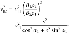
 (5)with
the compression ratio
s = ρ2/ρ1 = U1/U2.
Using these relations, the individual particle velocity components on the upstream and
downstream sides may be transformed into each other by
(5)with
the compression ratio
s = ρ2/ρ1 = U1/U2.
Using these relations, the individual particle velocity components on the upstream and
downstream sides may be transformed into each other by
 (6)and
 (7)To
simplify further evaluations, we introduce the abbreviations
(7)To
simplify further evaluations, we introduce the abbreviations  (8)and
 (9)i.e.
 and
and
 . Combining both
results, we find that
. Combining both
results, we find that  (10)Introducing
the ion pitch angle
β = ∠(v,n),
we obtain
(10)Introducing
the ion pitch angle
β = ∠(v,n),
we obtain 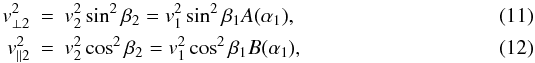 and
and
![Mathematical equation: \begin{equation} v_{2}^{2} = v_{1}^{2} \left[\sin^{2} \beta_{1} A(\alpha) + \cos^{2} \beta_{1} B(\alpha) \right], \label{eq-v1v2} \end{equation}](/articles/aa/full_html/2011/03/aa15619-10/aa15619-10-eq66.png) (13)which allows us to derive
the new dynamically associated downstream ion pitch-angle β2
as a function of upstream parameters
(13)which allows us to derive
the new dynamically associated downstream ion pitch-angle β2
as a function of upstream parameters  (14)Another simplification
that we use in the following sections is
(14)Another simplification
that we use in the following sections is
 (15)i.e.
  (16)
(16)
2.2. The distribution function at standing shocks
Using these results for individual particles, we derive the downstream distribution
function. Using Eqs. (11) and (12) and also Liouville’s equation (i.e.
continuity of the differential phase space flux at the jump), the connection between the
distribution functions upstream and downstream can be derived to be  (17)where
 is the initial downstream ion
distribution function, before pitch-angle isotropisation starts to dominate the system.
This intermediate distribution function is in most cases unstable with respect to plasma
instabilities and will trigger wave generation (Fahr
& Siewert 2007, 2008; Siewert & Fahr 2008; Fahr & Siewert 2010b). From Eqs. (13) and (17), it then
follows that
is the initial downstream ion
distribution function, before pitch-angle isotropisation starts to dominate the system.
This intermediate distribution function is in most cases unstable with respect to plasma
instabilities and will trigger wave generation (Fahr
& Siewert 2007, 2008; Siewert & Fahr 2008; Fahr & Siewert 2010b). From Eqs. (13) and (17), it then
follows that  may be expressed by
 (18)From Eq. (11), it follows that
 (19)while differentiating
Eq. (14) results in
(19)while differentiating
Eq. (14) results in
 (20)or
 (21)which results in
 (22)Therefore,
Eq. (18) transforms into
(22)Therefore,
Eq. (18) transforms into  (23)Finally, using
Eqs. (5) and (13) we find that
(23)Finally, using
Eqs. (5) and (13) we find that
 (24)where
we have used Eqs. (8) and (9), from which it follows that
(24)where
we have used Eqs. (8) and (9), from which it follows that
 . In other words, only the phase
space variables and not the distribution function itself are modified for the shock, which
agrees with earlier results by Siewert & Fahr
(2008).
. In other words, only the phase
space variables and not the distribution function itself are modified for the shock, which
agrees with earlier results by Siewert & Fahr
(2008).
2.3. Isotropic distributions
An even simpler form of this expression may be derived by assuming that
 quickly
returns to exhibiting pitch-angle isotropy because of effective pitch-angle scattering
processes on both sides of the jump. Using these additional assumptions, the velocity
transformation (Eq. (18)) takes the form
quickly
returns to exhibiting pitch-angle isotropy because of effective pitch-angle scattering
processes on both sides of the jump. Using these additional assumptions, the velocity
transformation (Eq. (18)) takes the form
![Mathematical equation: \begin{equation} \begin{split} v_{2}^{2} &=\,v_{1}^{2}\frac{1}{2} \int_0^\pi \sin\beta {\rm d}\beta \left[ \sin^2\beta A(\alpha_1) + \cos^2\beta B(\alpha_1) \right] \\ &=\,v_{1}^{2} \left[ \frac{2}{3} A(\alpha_1) + \frac{1}{3} B(\alpha_1) \right]. \end{split} \end{equation}](/articles/aa/full_html/2011/03/aa15619-10/aa15619-10-eq83.png) (25)Introducing,
again, a factor of C (analoguous to Eq. (16)), we obtain
(25)Introducing,
again, a factor of C (analoguous to Eq. (16)), we obtain  (26)This result then allows
us to write down a generalised formulation of the Liouville equation (similar to
Eq. (17), but for isotropic
distributions)
(26)This result then allows
us to write down a generalised formulation of the Liouville equation (similar to
Eq. (17), but for isotropic
distributions)  (27)From this
equation, it easily follows that
(27)From this
equation, it easily follows that  (28)and
further that
(28)and
further that  (29)
(29)
3. Theoretical treatment of travelling shocks
3.1. A toy model for consecutive travelling bulk velocity jumps
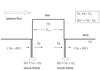 |
Fig. 1 The general form of a travelling shock induced by a nonlinear electrostatic double-soliton structure. |
We now attempt to apply the result derived above to the fairly equivalent situation of travelling shocks, i.e. travelling structures of bulk velocity jumps in the solar wind (e.g. see observations presented by Richardson et al. 2008).
We assume a jump contour (sketched in Fig. 1) with an upstream bulk velocity U1 and a downstream velocity U2, which in contrast to classical standing shock waves, are both assumed to be supersonic, i.e., U1,U2 ≫ cs, and that ΔU = U1 − U2 ≪ cs ≪ U1,U2 is the velocity at which the structure moves outwards with the solar wind. In this configuration, we now have travelling shock frames with a propagating static jump structure, i.e., frames moving with a velocity ΔU = U1 − U2, where at synchronously moving boundaries two opposite types of jumps by ΔU = ± U can occur.
These bulk velocity jumps may physically be envisioned to be caused by a nonlinear
electrostatic soliton composed of a superposition of electrostatic waves for which
k ∥ E ∥ U
with dispersion and dissipation (see Spatschek
1990; Infeld & Rowlands 1990) that
propagates with a velocity ΔU through a monokinetic plasma bulk flow.
Wherever this soliton arrives, it triggers a bulk velocity jump according to
 (30)over a distance
increment of
Δr = r2 − r1.
The opposite soliton with
E∗ (r − μSt) = −E(r − μSt)
and an identical wave profile propagates with the same group velocity
μS = ΔU, but wherever it arrives, it
decelerates the plasma flow by ΔU∗ = −ΔU
switching the bulk velocity back to its earlier value.
(30)over a distance
increment of
Δr = r2 − r1.
The opposite soliton with
E∗ (r − μSt) = −E(r − μSt)
and an identical wave profile propagates with the same group velocity
μS = ΔU, but wherever it arrives, it
decelerates the plasma flow by ΔU∗ = −ΔU
switching the bulk velocity back to its earlier value.
For demonstration purposes, we adopt jump conditions which we use in the following
sections of this paper given by 
3.2. Evolution of distribution functions at repeated travelling shock passings
Using our earlier results for standing shock waves, it is trivial to generalise
Eq. (24) to moving shock waves. Repeating our earlier results,
the intermediate (pre-isotropisation) downstream distribution function is given by
 (31)where
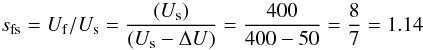
sfs is the fast-to-slow compression ratio defined by
(31)where
sfs is the fast-to-slow compression ratio defined by
 (32)After some time
τ = L/ΔU, this distribution
function will be re-integrated (or back-shuffled) into the fast bulk motion
Uf at the position of the reverse travelling shock (i.e.
induced by the reverse electrostatic soliton). Requesting again the conservation of the
two kinetic invariants, we may apply our formalism again and now obtain
(32)After some time
τ = L/ΔU, this distribution
function will be re-integrated (or back-shuffled) into the fast bulk motion
Uf at the position of the reverse travelling shock (i.e.
induced by the reverse electrostatic soliton). Requesting again the conservation of the
two kinetic invariants, we may apply our formalism again and now obtain
 (33)where we have
introduced to convert vs again into
vf the slow-to-fast compression ratio (see
also Sect. 4)
(33)where we have
introduced to convert vs again into
vf the slow-to-fast compression ratio (see
also Sect. 4)  (34)As we demonstrate
in Appendix A, the velocity components after
crossing both shock structures remain identical, i.e. particles return to their initial
phase space position after crossing the double structure, if the dynamical invariants
given by Eqs. (1) and (2) are conserved at both passages and
in-between. Therefore, no significant modification of the initial distribution function is
expected after n passings if the invariants are constantly conserved (but
see Sect. 4.4 for the description of a mechanism to
change this).
(34)As we demonstrate
in Appendix A, the velocity components after
crossing both shock structures remain identical, i.e. particles return to their initial
phase space position after crossing the double structure, if the dynamical invariants
given by Eqs. (1) and (2) are conserved at both passages and
in-between. Therefore, no significant modification of the initial distribution function is
expected after n passings if the invariants are constantly conserved (but
see Sect. 4.4 for the description of a mechanism to
change this).
A different result is obtained for the isotropic, pitch-angle scattering-processed
distribution function, (i.e. jump passage and isotropisation). Using Eq. (29), we obtain
 (35)This
result is different from the anisotropic case and results in an observable modification of
the reconverted ion distribution function with respect to the initial one. This result may
be generalised to an arbitrary number of repeating soliton-antisoliton crossings by noting
that the results for one twin-structure crossing are essentially identical to those for
the i-th crossing in a long chain of soliton-antisoliton passages, i.e.
(35)This
result is different from the anisotropic case and results in an observable modification of
the reconverted ion distribution function with respect to the initial one. This result may
be generalised to an arbitrary number of repeating soliton-antisoliton crossings by noting
that the results for one twin-structure crossing are essentially identical to those for
the i-th crossing in a long chain of soliton-antisoliton passages, i.e.
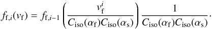 (36)This equation can
easily be transformed into a non-iterative form for i crossings,
resulting in
(36)This equation can
easily be transformed into a non-iterative form for i crossings,
resulting in 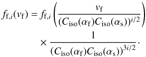 (37)Equation (37) illustrates an interesting property. The isotropic shock
introduces an additional normalising factor,
(C(αf)C(αs)) − 3i/2,
which is always positive and always either larger or smaller than 1 for all
i. This means that the behaviour of the distribution function (i.e. its
narrowing or broadening) can be derived by studying the behaviour of one single iteration.
(37)Equation (37) illustrates an interesting property. The isotropic shock
introduces an additional normalising factor,
(C(αf)C(αs)) − 3i/2,
which is always positive and always either larger or smaller than 1 for all
i. This means that the behaviour of the distribution function (i.e. its
narrowing or broadening) can be derived by studying the behaviour of one single iteration.
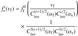
For completeness, we also derive an equivalent formulation for the slow plasma flow, i.e.
the distribution function emerging after i crossings of a double
fast-to-slow-to-fast structure, followed by one final fast-to-slow crossings. From
Eqs. (31) and (37), it then follows that
 (38)
(38)
4. Study of typical results
We now study the behaviour of these equations when applying them to typical initial
distribution functions. Using as standard values, the velocity fluctuations adopted in
Sect. 3.1, we obtain
 (39)and
 (40)
(40)
4.1. The development of an initial Maxwell-Boltzmann distribution
We start from an isotropic, upstream Maxwellian in the reference frame of the fast bulk
flow, i.e. ![Mathematical equation: \begin{equation} f_{\rm f,0} = \Phi_0 \exp \left[-\frac{mv_{\rm f}^{2}}{2kT_{\rm f,0}} \right] = \Phi_0 \exp [-\Gamma _{\rm f,0}v_{\rm f}^{2}], \label{eq-maxwell} \end{equation}](/articles/aa/full_html/2011/03/aa15619-10/aa15619-10-eq118.png) (41)where the subscript 0
denotes the initial upstream temperature parameter value of the initial ion population,
before the first crossing of a jump structure, and Φ0 is the initial
normalisation of the Maxwellian. This initial ion population can be represented by pick-up
ions implanted into the bulk flow by freshly ionized H-atoms, implying that
Tf,0 is given by
(41)where the subscript 0
denotes the initial upstream temperature parameter value of the initial ion population,
before the first crossing of a jump structure, and Φ0 is the initial
normalisation of the Maxwellian. This initial ion population can be represented by pick-up
ions implanted into the bulk flow by freshly ionized H-atoms, implying that
Tf,0 is given by  . (This
model results in a configuration where a new initial, “pristine” ion population is
generated continuously, and in addition to any non-initial population that has already
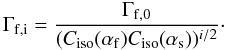
crossed multiple jump structures.) Equation (37) then leads to the
isotropic downstream ion distribution function, after crossing i soliton
structures given by
. (This
model results in a configuration where a new initial, “pristine” ion population is
generated continuously, and in addition to any non-initial population that has already
crossed multiple jump structures.) Equation (37) then leads to the
isotropic downstream ion distribution function, after crossing i soliton
structures given by ![Mathematical equation: \begin{equation} \begin{split} f_{\rm f,i}(v_{\rm s},\beta_{\rm s}) =&\, \Phi_0 \exp \left[-\Gamma_{\rm f} \frac{v_{\rm s}^{2}}{(C_{\rm iso}(\alpha_{\rm f})C_{\rm iso}(\alpha_{\rm s}))^i} \right] \\ & \times \frac{1}{\left(C_{\rm iso}(\alpha_{\rm f}) C_{\rm iso}(\alpha_{\rm s})\right)^{3i/2}} \\ =&\, \Phi_{\rm i} \exp \left[-\Gamma_{\rm f} \frac{v_{\rm s}^{2}}{(C_{\rm iso}(\alpha_{\rm f})C_{\rm iso}(\alpha_{\rm s}))^i} \right], \end{split} \end{equation}](/articles/aa/full_html/2011/03/aa15619-10/aa15619-10-eq123.png) (42)where
we have introduced the abbreviations
(42)where
we have introduced the abbreviations  (43)and
 (44)In other words, since
T ∝ Γ-1, we can see that with an increasing normalisation
factor, the temperature decreases, i.e. a narrowing distribution function correlates with
an increasing maximum, and vice versa.
(44)In other words, since
T ∝ Γ-1, we can see that with an increasing normalisation
factor, the temperature decreases, i.e. a narrowing distribution function correlates with
an increasing maximum, and vice versa.
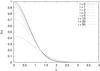 |
Fig. 2 Distribution functions after i individual pumping processes according to Eq. (37) for a perpendicular magnetic field. |
For the standard values adopted in our studies and a perpendicular shock (i.e.
αf = αs = 90°), we find that
 , and
hence,
, and
hence, 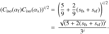 (45)Adopting
 as a lower limit for
sfs, we see that the expression in Eq. (45) is always larger than 1, i.e. the maximum (which coincides with the norm) of
the distribution function shrinks as the temperature of the new population grows.
Physically, this corresponds to an entropy increase, which demonstrates that the
underlying mechanism provides a valid heating process, which might be dubbed “pumped
heating”.
as a lower limit for
sfs, we see that the expression in Eq. (45) is always larger than 1, i.e. the maximum (which coincides with the norm) of
the distribution function shrinks as the temperature of the new population grows.
Physically, this corresponds to an entropy increase, which demonstrates that the
underlying mechanism provides a valid heating process, which might be dubbed “pumped
heating”.
Typical results for an initial Maxwellian with Γ0 = 1, αf = αs = 90°, and sfs = 1.14 are presented in Fig. 2, where one can easily observe the temperature increase as the broadening of the distribution function. The evolution of the temperature as a function of the counting index i is given in Fig. 3, while Fig. 4 demonstrates the difference between the initial, slow, and fast distribution functions at one individual double-jump structure.
4.2. Distribution functions in the presence of continuous reinjection of the initial distribution
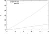 |
Fig. 3 Temperature parameter 1./Γ as a function of the number of pumping processes for perpendicular and parallel magnetic fields. |
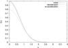 |
Fig. 4 Distribution functions at a double jump-structure. Depicted are the initial (pristine) function as well as the processed function after crossing the first half (deceleration) and both parts of a double-jump structurere-acceleration). |
![Mathematical equation: \begin{equation} f_{\rm f,final}(v) = \sum_{i} \Phi_{{\rm f},i} \cdot \exp [-v^{2} \Gamma_{{\rm f},i}]. \end{equation}](/articles/aa/full_html/2011/03/aa15619-10/aa15619-10-eq134.png) (46)If we assume that there
is a significant distance between the fast-to-slow and the slow-to-fast transitions, then
the slow distribution functions also need to be taken into account, resulting in the
additional contribution
(46)If we assume that there
is a significant distance between the fast-to-slow and the slow-to-fast transitions, then
the slow distribution functions also need to be taken into account, resulting in the
additional contribution ![Mathematical equation: \begin{equation} f_{\rm s}(v) = s_{\rm fs}\sum_{i} \frac{ \Phi_{{\rm s},i} }{ C_{\rm iso}(\alpha_{\rm f}) } \exp \left[-v^{2}\frac{\Gamma_{{\rm f},i}}{\sqrt{C_{\rm iso}(\alpha_{\rm f})}}\right]\cdot \end{equation}](/articles/aa/full_html/2011/03/aa15619-10/aa15619-10-eq135.png) (47)This interestingly enough
reflects the well-established finding in observational data that the spectral intensities
of ion distributions are inversely proportional to the bulk velocity of the solar wind
(Hill et al. 2009; Dayeh et al. 2009b; Simunac et al. 2009).
(47)This interestingly enough
reflects the well-established finding in observational data that the spectral intensities
of ion distributions are inversely proportional to the bulk velocity of the solar wind
(Hill et al. 2009; Dayeh et al. 2009b; Simunac et al. 2009).
In addition, we recall from Schwadron et al.
(2010) that a suitable superposition of Maxwellians with an entropy-maximising
weight function
F(λ) = exp( − λ/λ0)
leads to Kappa functions, and in the limit of
v2 ≫ λ0 to power laws
according to 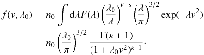 (48)Since
λ = Γf,i, this requirement for
F(λ) implies that,
(48)Since
λ = Γf,i, this requirement for
F(λ) implies that,
 (49)where we have skipped the
subscript i for the conversion between a discrete sum and a continuous
integral. Using Eqs. (43) and (44), we find that
(49)where we have skipped the
subscript i for the conversion between a discrete sum and a continuous
integral. Using Eqs. (43) and (44), we find that
 (50)This result
differs significantly from the exponential requirement, proving that the mechanism derived
here, while physically highly interesting, is unable to provide the configuration required
by Schwadron et al. (2010).
(50)This result
differs significantly from the exponential requirement, proving that the mechanism derived
here, while physically highly interesting, is unable to provide the configuration required
by Schwadron et al. (2010).
4.3. The development of an initial power-law distribution
Even though our proposed mechanism does not automatically result in the emergence of
power-law distribution functions, it is nevertheless of high interest to study how
existing power-law distribution functions are modified by the bulk velocity fluctuations
that have been studied before. Starting with an initially isotropic distribution function
of the form  (51)it follows from
Eq. (37) that
(51)it follows from
Eq. (37) that
 (52)This
result proves two different points. First, the powerlaw index will always be conserved,
supporting earlier results by Siewert & Fahr
(2008), who proved that power-law indices should be conserved because of the
results obtained at the termination shock. The second important consideration is the
behaviour of the normalising factor, which is either growing (for
κ > 3) or shrinking (for κ < 3) according
to the numerical value of κ.
(52)This
result proves two different points. First, the powerlaw index will always be conserved,
supporting earlier results by Siewert & Fahr
(2008), who proved that power-law indices should be conserved because of the
results obtained at the termination shock. The second important consideration is the
behaviour of the normalising factor, which is either growing (for
κ > 3) or shrinking (for κ < 3) according
to the numerical value of κ.
4.4. A new equilibrum state
We assume that a permanent back- and forth-shuffling of ions from fast-velocity to
slow-velocity bulk regimes and back takes place, where the size of the fluctuation
ΔU and the resulting compression ratios
 do not vary signifcantly, which means that a new equilibrium state can be expected to
arise from this process. This equilibrium would be reached if the distribution function of
the ions is no longer modifiedwhile a crossing of ions from the upstream to downstream and
back to the upstream side occurs, i.e. when
fi + 1(v) = fi(v)
is valid, or
do not vary signifcantly, which means that a new equilibrium state can be expected to
arise from this process. This equilibrium would be reached if the distribution function of
the ions is no longer modifiedwhile a crossing of ions from the upstream to downstream and
back to the upstream side occurs, i.e. when
fi + 1(v) = fi(v)
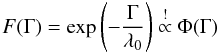
is valid, or  (53)The requested
special and appropriate equilibrum distribution function
f(v) is given in implicit form by this above
requirement. As suggested by the previous study of power laws, one solution of this
equation may be obtained by a power law approach, i.e.
f(v) = nv − κ,
which according to Eq. (53) results in the
requirement
(53)The requested
special and appropriate equilibrum distribution function
f(v) is given in implicit form by this above
requirement. As suggested by the previous study of power laws, one solution of this
equation may be obtained by a power law approach, i.e.
f(v) = nv − κ,
which according to Eq. (53) results in the
requirement  (54)leading
to
(54)leading
to  (55)which requires that
κ = 3. This result proves that any astrophysical plasma flow
encountering multiple shock-like fluctuations will ultimately take the form of a power-law
distribution with a power index of − κ = −3, which, interestingly,
neither depends on the fluctuation amplitude δU nor the magnetic tilt
angles α, obviously meaning that this equilibrium state is widely
insensitive to the specific plasma conditions.
(55)which requires that
κ = 3. This result proves that any astrophysical plasma flow
encountering multiple shock-like fluctuations will ultimately take the form of a power-law
distribution with a power index of − κ = −3, which, interestingly,
neither depends on the fluctuation amplitude δU nor the magnetic tilt
angles α, obviously meaning that this equilibrium state is widely
insensitive to the specific plasma conditions.
On the other hand, it must clearly be stated that this power index of − κ = −3 is different from the one most often found in space plasmas (see Gloeckler 2003; Fisk & Gloeckler 2006, 2007, 2008; Hill et al. 2009; Popecki et al. 2010; Dayeh et al. 2009a,b), namely −4.4 ≥ − κ ≥ − 6.6. This may perhaps be explained by varying our model assumptions, namely the assumption of rapid isotropisation. This interesting bridge between observations and the above formulated theoretical requirements may be to assume that the ions swept into the new bulk regime do not have enough time to isotropize completely, before they are re-incorporated into the consecutive other bulk, induced by a reverse jump. In this case, we are faced with a distribution function composed of an isotropic part and an anisotropic one. As we demonstrate in Appendix A of this paper, the ions that do not undergoing any pitch-angle isotropisation before being re-incorporated into the earlier bulk regime are re-integrated precisely with their original velocity components, i.e. no entropy is generated by this component of the system. Only the ions that have been isotropized before re-integration change the distribution function in the other bulk regime upon re-integration according to the relations developed in the paragraphs above.
We now ask in which sense this envisioned off-equilibrium state may change our earlier
results. First, we introduce the isotropisation ratio
ϵ = niso/ntot,
which defines how many ions successfully undergo the isotropisation process before they
encounter the next bulk velocity jump structure. To generate an observable power law, the
convergence of the system towards the equilibrum state must be sufficiently fast, i.e.
after a finite number of shock transitions. Now, accepting these assumptions, our modified
implicit equation is given by  (56)which
for a power law with spectral index
(56)which
for a power law with spectral index  leads to the requirement
  (57)resulting
in the solution
(57)resulting
in the solution 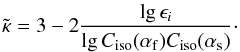 (58)This power-law index
 is mildly (logarithmically) dependent on the conditions of the bulk jump. Assuming, as an
example, a perpendicular jump, i.e. a jump with
α = π/2 and the standard values given in Sect. 4 (i.e. s = 1.17), it follows from
Eq. (45) that
C(90°)C(90°) ≃ 1.0055. Thus, one finds that
is mildly (logarithmically) dependent on the conditions of the bulk jump. Assuming, as an
example, a perpendicular jump, i.e. a jump with
α = π/2 and the standard values given in Sect. 4 (i.e. s = 1.17), it follows from
Eq. (45) that
C(90°)C(90°) ≃ 1.0055. Thus, one finds that
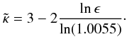 (59)Plotting this
equation as a function of ϵ, Fig. 5
then allows us to estimate the conditions under which for residual pitch-angle
anisotropies an average value of
(59)Plotting this
equation as a function of ϵ, Fig. 5
then allows us to estimate the conditions under which for residual pitch-angle
anisotropies an average value of  is reached. From this figure, it
follows that the stable power-law index κ strongly on the plasma jump
parameters, although in general, only small anisotropy values
0.95 ≤ ϵ ≤ 1 result in power-law indices in the regime of commonly
observed values, i.e. −4.4 ≳ − κ ≳ −6.6. This result suggests that
realistic power-law indices observed in astrophysical systems may be stabilised by local
bulk velocity fluctuations in the presence of a small (i.e. ≲ 5 − 10%) temperature (i.e.
pitch-angle) anisotropy. This result agrees well with the observational finding that the
solar wind plasma in general may be considered as isotropic, although with just the small
kind of fluctuations appearing in any realistic system because of local derivations from
an ideal configuration.
is reached. From this figure, it
follows that the stable power-law index κ strongly on the plasma jump
parameters, although in general, only small anisotropy values
0.95 ≤ ϵ ≤ 1 result in power-law indices in the regime of commonly
observed values, i.e. −4.4 ≳ − κ ≳ −6.6. This result suggests that
realistic power-law indices observed in astrophysical systems may be stabilised by local
bulk velocity fluctuations in the presence of a small (i.e. ≲ 5 − 10%) temperature (i.e.
pitch-angle) anisotropy. This result agrees well with the observational finding that the
solar wind plasma in general may be considered as isotropic, although with just the small
kind of fluctuations appearing in any realistic system because of local derivations from
an ideal configuration.
5. Conclusion
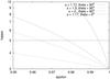 |
Fig. 5 Stable values for the power law index |
We have demonstrated that a chain of bulk velocity jumps passing over a co-moving ion
population under two specific conditions automatically leads to power law velocity
distribution functions. The first condition is that the two particle invariants introduced
in this paper are conserved at bulk velocity jumps, and the second that between the periods
of the passage of two consecutive bulk velocity jumps the jump-induced initially anisotropic
distribution is again isotropized rapidly enough by pitch-angle scattering. For these
conditions, we have shown that a power-law distribution develops as an equilibrium ion
distribution function with a spectral velocity power index of −κ = −3.
Spectral indices of −4.4 ≥ − κobs ≥ −6.6 as often found by
plasma analysers in heliospheric space plasmas (see e.g. Gloeckler 2003; Dayeh et al. 2009b; Desai et al. 2010) can be obtained in the framework of the
aforementioned theory, if only partial, incomplete isotropisation of the ion distribution
has taken place, before the next bulk velocity jump passage occurs. When incomplete
isotropisation occurs within the period of one bulk regime passage, i.e.
τU = LU/ΔU,
where the quantity LU is the one-dimensional
extent of a mono-bulk regime, with only a percentage ϵ of ions becoming
isotropized, the resulting power index will become larger. This covers the observationally
found power indices at 0.95 ≲ ϵ ≲ 1, with
 for an isotropisation degree of
ϵ ≃ 0.99.
for an isotropisation degree of
ϵ ≃ 0.99.
On the other hand, we have to admit here that the above study was carried out for somewhat idealistic one-dimensional plasma flow conditions with no plasma flow divergence in the flow direction (i.e. no radially symmetric outflow). In reality, the solar wind plasma flow to first order is spherically symmetric with a flow divergence in the radial flow direction that leads to the magnetic or adiabatic cooling of ions (see Fahr 2007; Fahr & Siewert 2008) convected outwards to larger radial distances. The cooling of co-convected ions is due to both a differential bulk drift and the conservation of the magnetic moment in a flow with decreasing magnetic field magnitude and results in a velocity magnitude drift towards smaller particle velocities. As we have shown in Fahr & Siewert (2008), this leads to (−5)-power-law ion distributions for ion velocities v ≤ U of pick-up ions injected at the injection border of v = U. If this effect were to be appropriately taken into account, then instead of a Maxwellian with Tf0 = mU2/3K as taken in Eq. (41), one would start instead from an initial power-law function with − κ = −5, an initial upper velocity border of v = U and a lower velocity border of v ≃ U [1 − (U/ΔU)(LU/r) ] , and then process this function by jump crossings.
In this context, we note that when studying the influence of bulk velocity fluctuations on ion distribution functions for the general Parker phase space transport equation when cooling processes are not taken into account, Zhang (2010) derived velocity power laws with a spectral index of −κZ = −3. In his study, it is suspected that adequate consideration of cooling processes in the framework of his theory would result in softer power-law spectra with −κ ≃ −5. This may allow the conclusion that bulk velocity fluctuations naturally lead to power laws, but only then to those with actually observed power indices, if the effects of ion cooling and incomplete isotropisation of distribution functions are properly taken into account, as we propose to study in the near future.
In the energizing process that has been studied in this paper, the energy arriving in the suprathermal power-law tails is generated by entropy production from the free energy sitting in the differential kinetic energies of succeeding bulk velocity jumps. The entropisation needed only occurs through isotropisation of the initially anisotropic distribution function (see Fahr & Siewert 2010a) appearing immediately after jump passage where dynamical ion invariants are conserved. When no complete isotropisation is granted, off-equilibrium ion spectra with spectral velocity power indices of κv ≤ −3 have to be expected.
The fully developed equilibrium that we have described in Sect. 4.4 is of course somewhat artificial, but represents the asymptotic state towards which the system would tend, if all competing processes (especially cooling processes) run slow. In our approximation, we have taken into account no cooling processes that, however, operate unavoidably in a radially diverging plasma flow and tend to steepen the spectra towards spectral indices κv ≤ −3.
On the other hand, too high a pressure should not be a problem in the context of quasi-equilibrum ion power laws, since a natural upper velocity border always exists up to which the process we are studying here can operate. Only these ions can conserve their dynamical invariants at the crossing over the bulk velocity jump with subcritical velocities v ≤ vc (for a definition see Eq. (60)). At higher velocities v ≥ vc, ions become free to escape by spatial diffusion from the jump structure and thereby do not conserve ion invariants. These particles thus stop participating in the pumping process due to bulk velocity jumps (i.e. compressive turbulence), thereby defining a roll-over and causing at supercritical ion velocities a fall-off of the ion spectrum to spectral slopes κv ≤ −5 that keep the ion pressure finite.
Furthermore, at the end of this paper, we need to come back to the point raised in the
beginning, namely that conservation of those particle invariants used in the aforementioned
derivations can only be expected to hold for ions with subcritical velocities
 , i.e. ions that cannot escape
from the jump structure by spatial diffusion while undergoing jump-induced velocity
transformation with conserved invariants. If passage times of the jump structure and
diffusion times become comparable, i.e. if
, i.e. ions that cannot escape
from the jump structure by spatial diffusion while undergoing jump-induced velocity
transformation with conserved invariants. If passage times of the jump structure and
diffusion times become comparable, i.e. if 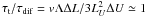 , then ions can effectively escape
from the jump structure without conserving the applied invariants. This then leads to an
upper validity border of
, then ions can effectively escape
from the jump structure without conserving the applied invariants. This then leads to an
upper validity border of  (60)where
 evaluates
to vc ≃ 3.75 × 10³U. This indicates
that the theory presented here does not apply to high ion velocities with
v ≥ vc. At these energies, the theoretical
approach presented by Fisk & Gloeckler (2006,
2007, 2008)
instead applies which, however, as also in our equilibrum case, has to rely on completely
isotropic ion distributions.
evaluates
to vc ≃ 3.75 × 10³U. This indicates
that the theory presented here does not apply to high ion velocities with
v ≥ vc. At these energies, the theoretical
approach presented by Fisk & Gloeckler (2006,
2007, 2008)
instead applies which, however, as also in our equilibrum case, has to rely on completely
isotropic ion distributions.
Acknowledgments
One of the authors, M. Siewert, is grateful to the Deutsche Forschungsgemeinschaft for financial support granted to him in the frame of the project Si-1550/2-1.
This research benefited greatly from discussions that were held at the meetings of the International Team devoted to understanding the − 5 tails and ACRs that has been sponsored by the International Space Science Institute in Bern, Switzerland.
References
- Chalov, S. V. 2005, Adv. Space Res., 35, 2106 [NASA ADS] [CrossRef] [Google Scholar]
- Chalov, S. V., Fahr, H.-J., & Izmodenov, V. 1997, A&A, 320, 659 [NASA ADS] [Google Scholar]
- Chew, G. F., Goldberger, M. L., & Low, F. E. 1956, Proc. R. Soc. London A, 236, 112 [Google Scholar]
- Dayeh, M. A., Desai, M. I., Dwyer, J. R., et al. 2009a, ApJ, 693, 1588 [Google Scholar]
- Dayeh, M. A., Desai, M. I., Kozarev, K. A., et al. 2009b, AGU Fall Meeting Abstracts, A1492 [Google Scholar]
- Decker, R. B., Krimigis, S. M., Roelof, E. C., et al. 2005, Science, 309, 2020 [NASA ADS] [CrossRef] [PubMed] [Google Scholar]
- Decker, R. B., Krimigus, S. M., Roelof, E. C., et al. 2008, Nature, 454, 67 [NASA ADS] [CrossRef] [PubMed] [Google Scholar]
- Desai, M. I., Dayeh, M. A., & Mason, G. M. 2010, Twelfth International Solar Wind Conference, 1216, 635 [NASA ADS] [Google Scholar]
- Diver, D. A. 2001, A Plasma Formulary for Physics, Technology and Astrophysics (Hoboken, New Jersey: John Wiley) [Google Scholar]
- Erkaev, N. V., Vogl, D. F., & Biernat, H. K. 2000, J. Plasma Physics, 64, 561 [Google Scholar]
- Fahr, H.-J. 2007, Ann. Geophys., 25, 2649 [NASA ADS] [CrossRef] [Google Scholar]
- Fahr, H.-J., & Siewert, M. 2007, ASTRA, 3, 21 [NASA ADS] [CrossRef] [Google Scholar]
- Fahr, H.-J., & Siewert, M. 2008, A&A, 484, L1 [NASA ADS] [CrossRef] [EDP Sciences] [Google Scholar]
- Fahr, H.-J., & Siewert, M. 2009, ApJ, 693, 281 [NASA ADS] [CrossRef] [Google Scholar]
- Fahr, H.-J., & Siewert, M. 2010a, ASTRA, 7, 1 [Google Scholar]
- Fahr, H.-J., & Siewert, M. 2010b, A&A, 512, A64 [NASA ADS] [CrossRef] [EDP Sciences] [Google Scholar]
- Fichtner, H., Le Roux, J. A., Mall, U., & Rucinski, D. 1996, A&A, 314, 650 [NASA ADS] [Google Scholar]
- Fisk, L. A. 1976, J. Geophys. Res., 81, 4633 [Google Scholar]
- Fisk, L. A., & Gloeckler, G. 2006, ApJ, 640, L79 [NASA ADS] [CrossRef] [Google Scholar]
- Fisk, L. A., & Gloeckler, G. 2007, PNAS, 104, 5749 [NASA ADS] [CrossRef] [Google Scholar]
- Fisk, L. A., & Gloeckler, G. 2008, ApJ, 686, 1466 [NASA ADS] [CrossRef] [Google Scholar]
- Forsyth, R. J., Balogh, A., & Smith, E. J. 2002, J. Geophys. Res. (Space Physics), 107, 1405 [Google Scholar]
- Gloeckler, G. 2003, in Solar Wind Ten, ed. M. Velli, R. Bruno, F. Malara, & B. Bucci, AIP Conf. Ser., 679, 583 [Google Scholar]
- Gombosi, T. I. 1998, Physics of the Space Environment (New York: Cambridge University Press) [Google Scholar]
- Hill, M. E., Schwadron, N. A., Hamilton, D. C., Di Fabio, R. D., & Squier, R. K. 2009, ApJ, 699, L26 [NASA ADS] [CrossRef] [Google Scholar]
- Infeld, E., & Rowlands, G. 1990, Nonlinear Waves, Solitons and Chaos, ed. E. Infeld, & G. Rowlands [Google Scholar]
- Jokipii, J. R., & Lee, M. A. 2010, ApJ, 713, 475 [NASA ADS] [CrossRef] [Google Scholar]
- le Roux, J. A., & Fichtner, H. 1999, J. Geophys. Res., 104, 4709 [NASA ADS] [CrossRef] [Google Scholar]
- McComas, D. J., Barraclough, B. L., Funsten, H. O., et al. 2000, J. Geophys. Res., 105, 10419 [NASA ADS] [CrossRef] [Google Scholar]
- McComas, D. J., Elliott, H. A., Schwadron, N. A., et al. 2003, Geophys. Res. Lett., 30, 100000 [Google Scholar]
- Parker, E. N. 1958, ApJ, 128, 664 [Google Scholar]
- Parker, E. N. 1965, Plan. Sp. Sc., 13, 9 [NASA ADS] [CrossRef] [Google Scholar]
- Popecki, M., et al. 2010, Talk held at Tail-workshop at ISSI (Bern) [Google Scholar]
- Richardson, J. D., Wang, C., & Burlaga, L. F. 2003, Geophys. Res. Lett., 30, 2207 [NASA ADS] [CrossRef] [Google Scholar]
- Richardson, J. D., Liu, Y., Wang, C., & McComas, D. J. 2008, A&A, 491, 1 [NASA ADS] [CrossRef] [EDP Sciences] [Google Scholar]
- Schwadron, N. A., Dayeh, M. A., Desai, M., et al. 2010, ApJ, 1386 [Google Scholar]
- Siewert, M., & Fahr, H.-J. 2008, A&A, 485, 327 [NASA ADS] [CrossRef] [EDP Sciences] [Google Scholar]
- Simunac, K. D. C., Kistler, L. M., Galvin, A. B., et al. 2009, Sol. Phys., 259, 323 [Google Scholar]
- Spatschek, K.-H. 1990, Theoretische Plasmaphysik (Stuttgart: Teubner Verlag) [Google Scholar]
- Toptygin, I. N. 1983, Cosmic Rays in Interplanetary Magnetic Fields (Norwell/Mass.: D. Reidel Publ.) [Google Scholar]
- Treumann, R. A., & Baumjohann, W. 1997, Adv. Space Plasma Phys. (London: Imperial College Press) [Google Scholar]
- Zhang, M. 2010, J. Geophys. Res., 115, A12102 [NASA ADS] [CrossRef] [Google Scholar]
Appendix A: Immediate re-shuffling of downstream ions back into the upstream regime
Immediate re-shuffling of freshly generated slow-flow particles back into the fast bulk
(i.e. triggered for instance by a very sharp
E∗ − E −
double-soliton structure), without prior mixing of velocity components, would lead to the
velocity coordinate re-transformations
 (A.1)and
 (A.2)Now,
it follows from Eq. (5) that
(A.2)Now,
it follows from Eq. (5) that
 ; using
Eq. (34) reduces this to
; using
Eq. (34) reduces this to
 and
therefore,
and
therefore,  . From this result, it
immediately follows that
. From this result, it
immediately follows that  (A.3)or, using Eq. (8),
 (A.4)This equation allows us
to obtains the following complete identities from Eqs. (6)
and (7)
(A.4)This equation allows us
to obtains the following complete identities from Eqs. (6)
and (7)
 (A.5)and
 (A.6)meaning
that without stochastic or isotropizing processes on the downstream side the re-integrated
ions exactly re-constitute the upstream distribution function, i.e. they are completely
adiabatic and reversible.
(A.6)meaning
that without stochastic or isotropizing processes on the downstream side the re-integrated
ions exactly re-constitute the upstream distribution function, i.e. they are completely
adiabatic and reversible.
If, however, prior to re-shuffling into the other bulk frame mixing between the two degrees of freedom parallel and perpendicular to B, e.g. due to either wave generation or pitch-angle scattering, occurs, then the transformations undergo interesting irreversibilities, which we have studied in the main text.
All Figures
|
Fig. 1 The general form of a travelling shock induced by a nonlinear electrostatic double-soliton structure. |
| In the text | |
|
Fig. 2 Distribution functions after i individual pumping processes according to Eq. (37) for a perpendicular magnetic field. |
| In the text | |
|
Fig. 3 Temperature parameter 1./Γ as a function of the number of pumping processes for perpendicular and parallel magnetic fields. |
| In the text | |
|
Fig. 4 Distribution functions at a double jump-structure. Depicted are the initial (pristine) function as well as the processed function after crossing the first half (deceleration) and both parts of a double-jump structurere-acceleration). |
| In the text | |
|
Fig. 5 Stable values for the power law index |
| In the text | |
Current usage metrics show cumulative count of Article Views (full-text article views including HTML views, PDF and ePub downloads, according to the available data) and Abstracts Views on Vision4Press platform.
Data correspond to usage on the plateform after 2015. The current usage metrics is available 48-96 hours after online publication and is updated daily on week days.
Initial download of the metrics may take a while.