| Issue |
A&A
Volume 527, March 2011
|
|
|---|---|---|
| Article Number | A17 | |
| Number of page(s) | 14 | |
| Section | Astrophysical processes | |
| DOI | https://doi.org/10.1051/0004-6361/201015256 | |
| Published online | 19 January 2011 | |
Relativistic slim disks with vertical structure
1
Nicolaus Copernicus Astronomical Center, Polish Academy of
Sciences, Bartycka
18, 00-716
Warszawa,
Poland
e-mail: This email address is being protected from spambots. You need JavaScript enabled to view it.
; This email address is being protected from spambots. You need JavaScript enabled to view it.
; This email address is being protected from spambots. You need JavaScript enabled to view it.
2
Department of Physics, Göteborg University,
412-96
Göteborg,
Sweden
e-mail: This email address is being protected from spambots. You need JavaScript enabled to view it.
3
Astronomical Institute, Academy of Sciences of the Czech Republic,
Bočni II/1401a,
141-31
Prague, Czech
Republic
e-mail: This email address is being protected from spambots. You need JavaScript enabled to view it.
4
Institut d’Astrophysique de Paris, UMR 7095 CNRS, UPMC Univ. Paris 06,
98bis Bd
Arago, 75014
Paris,
France
e-mail: This email address is being protected from spambots. You need JavaScript enabled to view it.
5
Jagiellonian University Observatory, ul. Orla 171, 30-244
Kraków,
Poland
Received:
22
June
2010
Accepted:
6
November
2010
Abstract
We report on a scheme for incorporating vertical radiative energy transport into a fully relativistic, Kerr-metric model of optically thick, advective, transonic alpha disks. Our code couples the radial and vertical equations of the accretion disk. The flux was computed in the diffusion approximation, and convection is included in the mixing-length approximation. We present the detailed structure of this “two-dimensional” slim-disk model for α = 0.01. We then calculated the emergent spectra integrated over the disk surface. The values of surface density, radial velocity, and the photospheric height for these models differ by 20%–30% from those obtained in the polytropic, height-averaged slim disk model considered previously. However, the emission profiles and the resulting spectra are quite similar for both types of models. The effective optical depth of the slim disk becomes lower than unity for high values of the alpha parameter and for high accretion rates.
Key words: black holes physics / accretion, accretion disks
© ESO, 2011
1. Introduction
Modeling accretion flows onto black holes is crucial for understanding the energetic emissions observed from many sources, both Galactic and extragalactic (e.g., X-ray binaries, ULXs, AGNs). The accreting matter commonly settles into a disk-like configuration in which angular momentum is transported outwards as a result of shear in the differentially rotating fluid, allowing mass to be accreted onto the central compact object. Of particular interest are sources such as the low-mass X-ray binaries in which matter is transferred onto the X-ray source from a binary companion, usually a late-type star. When containing a black hole, these sources undergo irregular outbursts (lasting several months or years) that are analogous to the outbursts observed in dwarf novae, and are thought to be related to the viscous-thermal instability, which leads to an enhanced transfer of angular momentum in the accreting fluid (Lasota 2001).
In outburst, the source is a luminous X-ray emitter and as the luminosity decays from the outburst maximum to minimum, the disk is thought to follow a sequence of quasi-stationary states, whose spectra can be derived from steady-state models of accretion disks. At high luminosities describing the inner regions of such accretion disks by the most-often used “thin disk” models is no longer valid. A description of such disks in terms of “slim disk” models is more appropriate.
Following the approach of Shakura & Sunyaev (1973), in the “standard" discussion of stationary disk structure one assumes that there is no radial advection of heat (the flow is “radiatively efficient”), the radial pressure gradients are negligible, and the distribution of angular momentum is Keplerian. All of these assumptions hold for very thin disks, including the original Shakura & Sunyaev (1973) model (henceforth SS) and its general-relativistic version (NT), which was developed for the Kerr geometry by Novikov & Thorne (1973). However, it has long been realized that not all disk-like accretion flows satisfy these assumptions In particular, slim disks (e.g., Abramowicz et al. 1988) form a stable branch of accretion, in which advection of entropy is important and the disk is not necessarily geometrically thin. These solutions are particularly relevant to sources with high accretion rates, and they converge to the standard case in the low accretion rate limit.
In the case of thin disks, methods for treating the radiative transfer and computing the vertical structure of the disk have been developed by Shaviv & Wehrse (1986) and Hubeny (1998) and applied by, e.g., Davis & Hubeny (2006), Idan et al. (2008), and Różańska & Madej (2008). These have not yet been applied to slim disks. Until recently, the properties of slim disk models have been represented with quantities averaged over the vertical structure of the disk. This paper presents improved advective steady-state models of accretion, in which the vertical structure of the “slim disk” is explicitly taken into account.
Recently, Sądowski (2009) revisited slim disk models with an improved numerical code, while Sądowski et al. (2009) performed a preliminary study of the slim disk vertical structure. While our present work is based on these two papers, it breaks with the long tradition of computing the radial dependence of disk quantities, including the emergent flux F(r), before the vertical structure is analyzed. In this paper, by closely coupling the radial properties of the disk to its vertical structure, we offer a more consistent treatment of the slim disk. A similar approach has been taken by Dotan & Shaviv (2010) in their discussion of winds from Super-Eddington slim disks in a pseudo-Newtonian potential.
The high luminosities observed in the bright X-ray sources imply there is an effective mechanism of angular momentum transport in the accreting fluid, and much work has been devoted to MHD simulations of one such mechanism, the magneto-rotational instability (MRI). For thin disks, the effectiveness of angular momentum transport is conveniently parametrized by the alpha parameter that was introduced by Shakura & Sunyaev (1973). Observations of systems in which variability is driven by accretion disk instabilities suggest rather high values of α for fully ionized disks, much higher than the value α = 0.001 that was adopted in the original slim-disk article (Abramowicz et al. 1988). Smak (1999) has already showed that one has to take α ≈ 0.2 to describe hot disks in dwarf novae. As reviewed by King et al. (2007), the value of α in hot, fully ionized disks has to be ~0.1−0.4, whereas in cold protostellar and FU Urionis disks, much lower values of this parameter are required ~0.01 and ~0.001−0.003, respectively. Numerical simulations give a value of α ~ 0.01 for ionized disks, ten times lower than suggested by observations, and it probably reflects the limitations of the present MRI calculations (King et al. 2007). However, the apparently observational determinations of α mentioned above are in fact strongly model-dependent. In the case of dwarf-novae, for example, these determinations assume that outbursts are described well by the thermal-viscous instability model. However, the case of the epitome dwarf-nova SS Cyg shows that such a description might be inadequate (Schreiber & Lasota 2007; Smak 2010), putting presumably observational determinations into doubt. Therefore, one cannot exclude that the numerical simulations are correct after all.
In this paper we adopt the value α = 0.01. With such a low value of α, the resulting disk models are optically thick (τeff > 1), thus allowing a simplified treatment of radiative transfer. We treat the vertical energy transport in the diffusive approximation for the radiative flux (and account for vertical convection in the mixing-length approximation).
We begin the body of the paper with a brief discussion of the model, then both the radial and the vertical equations of disk structure are presented. In Sect. 3 we describe the numerical method used to solve the problem. The radial structure of the solutions is described in Sect. 4.1, while the vertical profiles of various disk quantities are discussed in Sect. 4.2. By comparing our results with previous work, we find that, with a judicious choice of parameters, a standard polytropic slim disk model can be made to approximate our full solution. Analytical formulae for the appropriate values of the parameters can be found in Sect. 5. Finally, in the last section we discuss the limitations of the model and its possible applications.
2. Slim-disk structure
Slim disks are alpha disks. Like Shakura-Sunyaev disks they are based on the assumption that the dissipation mechanisms operating in accretion flows may be described by a viscous stress tensor whose leading component is proportional to the pressure.
Slim disk solutions, again just like the SS and NT solutions, are obtained by solving vertically averaged (or height-integrated), radial equations of motion. Thus, steady slim disks, like the SS and NT ones, neglect the vertical structure of flow, and describe essentially flat fluid configurations. Although an expression for the radial dependence of disk thickness is obtained, the slope of the disk surface is usually neglected in the discussion of emergent spectra, where a plane-parallel atmosphere is typically considered for the purposes of computing radiative transfer in the vertical direction.
In the case of slim disks, the radial equations of structure are a set of ordinary differential equations (ODEs). For a detailed account of these Kerr-metric equations (and state-of-the-art traditional slim-disk models), see Sądowski (2009), who followed previous work beginning with Lasota (1994), and considered subsequent improvements (Abramowicz et al. 1996, 1997; Gammie & Popham 1998). The set of equations is closed by including relations describing vertical hydrostatic equilibrium and vertical transport of energy. By solving these equations with appropriate boundary (or regularity) conditions, one obtains the radial profiles of the central temperature, Tc(r), surface density, Σ(r), the height-integrated pressure, P(r), the half-thickness of the disk, h(r), a radial velocity V(r), the emerging flux of radiation, F(r), and certain other physical quantities.
In this paper we are taking a first step towards constructing truly three-dimensional slim disk models, by solving a set of differential equations describing the vertical structure of the disk. The resulting z-dependence of physical quantities is used to compute certain coefficients that enter the radial equations and that up till now have been estimated with algebraic expressions. We refer to the resulting models as “two-dimensional (2-D) slim disk” solutions, although it has to be understood that in contrast to the thin-disk solutions of Urpin (1984) and Kluźniak & Kita (2000), the actual meridional flow has not been computed in this paper, but the average radial velocity alone has been considered in the structure equations. However, the models are now self-consistent in the sense that the vertical averages of physical quantities that form the coefficients of the radial ODEs do correspond to the vertical structure considered in the radiative transfer calculation – in previous work the vertical structure of the radiative atmosphere was considered a posteriori, and it had no influence on the radial structure of the disk.
2.1. Basic assumptions, parameters, and coefficients
We assume an axially symmetric, stationary fluid configuration in the Kerr metric, with fixed values of the black hole (BH) mass, M, and spin, a, parameters and the fluid disk is symmetric under reflection in the equatorial plane of the metric. Matter is supplied at a steady rate, Ṁ, through a boundary “at infinity” and angular momentum is removed through the same boundary (in practice, we use the NT solution for the outer boundary condition), whereas zero torque is assumed at the BH horizon. We assume that no mass or angular momentum crosses the disk surface. We neglect the loss of angular momentum to both wind and radiation. We do not consider self-irradiation of the disk and assume that the magnetic pressure may be neglected. Neglecting the incoming radiation may not be justified for super-Eddington accretion rates for which the disk is geometrically thick.
A fraction, (1 + fadv(r))-1, of the entropy generated locally by dissipative processes is released into the radiation field, while the remainder is advected by the gas.
A unique solution to the slim-disk model can only be found if certain additional assumptions are made. We make the following arbitrary choice. We neglect the vertical variation (z dependence) of the velocity field, considering only its height-averaged value; thus, the velocity is always directed radially inwards and is a function of the radial coordinate alone. Similarly, we assume there is no z variation of the advection factor fadv(r). Dissipation and angular momentum transport are given by the alpha prescription (Shakura & Sunyaev 1973), with a constant value of α. We assume that the dissipation rate is proportional to the total pressure, p. For a more detailed statement, see Eq. (13) and the comment following it. Calculations are carried out for the value α = 0.01.
We are looking for 2-D slim-disk solutions at a definite value of mass accretion rate for a given Kerr metric. Thus, for a fixed value of α, there are three fundamental parameters describing a given slim-disk solution: M, a, and Ṁ.
In the structure equations, we take G = c = 1 and make
use of the following expressions involving the BH spin:
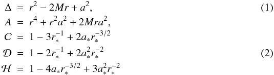 with
a∗ = a/M and
r∗ = r/M.
with
a∗ = a/M and
r∗ = r/M.
We use the Boyer-Lindquist system of coordinates and introduce the vertical coordinate
z = rcosθ. The metric near the
equatorial plane takes the form (Abramowicz et al.
1996),  (3)where
ω = 2Mar/A is the angular velocity
of the frame dragging.
(3)where
ω = 2Mar/A is the angular velocity
of the frame dragging.
The radial gas (three-)velocity, V, as measured by an observer
co-rotating with the fluid at a fixed value of r, is given by the
relation (Abramowicz et al. 1996) 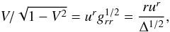 (4)where
ur is the contravariant radial component
of the fluid 4-velocity and has the dimension of physical velocity. The disk surface
density is
(4)where
ur is the contravariant radial component
of the fluid 4-velocity and has the dimension of physical velocity. The disk surface
density is  , while the height-integrated pressure is
 . The total pressure is the sum of gas and
radiation pressures,
p = pgas + prad.
We adopt an equation of state corresponding to the choice
pgas = kρT/(μmp),
and
prad = aT4/3,
with k the Boltzmann constant, mp the proton
mass, and a the radiation constant (no confusion with the spin parameter
may arise). The mean molecular weight is taken to be μ = 0.62, but see
the comment following Eq. (21). The
height-integrated energy density is
. The total pressure is the sum of gas and
radiation pressures,
p = pgas + prad.
We adopt an equation of state corresponding to the choice
pgas = kρT/(μmp),
and
prad = aT4/3,
with k the Boltzmann constant, mp the proton
mass, and a the radiation constant (no confusion with the spin parameter
may arise). The mean molecular weight is taken to be μ = 0.62, but see
the comment following Eq. (21). The
height-integrated energy density is
 (5)where
γ = 5/3.
(5)where
γ = 5/3.
The following averages (moments) enter the radial equations as coefficients of certain
terms:  All
integrals in this section are taken at a fixed value of r. Here,
T(z) is the gas temperature, and
Tc is its value at the equatorial plane,
T(0) = Tc.
All
integrals in this section are taken at a fixed value of r. Here,
T(z) is the gas temperature, and
Tc is its value at the equatorial plane,
T(0) = Tc.
The vertical epicyclic frequency squared, which can be thought of as the vertical
component of gravity, is (Kato 1993),  (10)We also define
 (11)
(11)
2.2. Vertical structure equations
We describe the vertical structure of an accretion disk in the optically thick regime by the following equations:
-
(i)
Hydrostatic equilibrium (Katoet al. 2008),
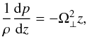 (12)where
Ω ⊥ is defined in Eq. (10). Although other expressions for the right-hand side of Eq. (12) can be found in the literature (e.g.,
Abramowicz et al. 1997, includes
vz ≠ 0), the form above is
appropriate for our scheme, in which the vertical structure is precalculated before
any information about the radial variables becomes available. Thus, in Eqs. (10) and (12), we assume Keplerian angular velocity
(12)where
Ω ⊥ is defined in Eq. (10). Although other expressions for the right-hand side of Eq. (12) can be found in the literature (e.g.,
Abramowicz et al. 1997, includes
vz ≠ 0), the form above is
appropriate for our scheme, in which the vertical structure is precalculated before
any information about the radial variables becomes available. Thus, in Eqs. (10) and (12), we assume Keplerian angular velocity
![Mathematical equation: $[M/({\cal C} r^3)]^{1/2}$](/articles/aa/full_html/2011/03/aa15256-10/aa15256-10-eq53.png) , as well as
vz = 0 in hydrostatic equilibrium.
, as well as
vz = 0 in hydrostatic equilibrium.
-
(ii)
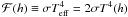
The energy generation equation. We assume that the vertical flux of energy inside the disk ℱ is generated according to
 (13)Strictly
speaking, this does not correspond to a constant α prescription, as
the term
(3/2)(M/r3)1/2,
which is derived from Keplerian strain, departs somewhat from the value that would
follow from the actually computed distribution of angular momentum (cf., Fig. 1). However, as the departure for sub-Eddingtonian
accretion rates is small, we expect Eq. (13) to afford a good approximation. Note that
fadv = 0 corresponds to the NT disk (going over into
the Shakura-Sunyaev disk in the nonrelativistic limit of thin disks),
fadv > 1 characterizes advection-dominated
disks, while fadv < 0 describes those disk
regions where the advected heat is being released. The amount of heat advected
Qadv = fadvℱ(h).
(13)Strictly
speaking, this does not correspond to a constant α prescription, as
the term
(3/2)(M/r3)1/2,
which is derived from Keplerian strain, departs somewhat from the value that would
follow from the actually computed distribution of angular momentum (cf., Fig. 1). However, as the departure for sub-Eddingtonian
accretion rates is small, we expect Eq. (13) to afford a good approximation. Note that
fadv = 0 corresponds to the NT disk (going over into
the Shakura-Sunyaev disk in the nonrelativistic limit of thin disks),
fadv > 1 characterizes advection-dominated
disks, while fadv < 0 describes those disk
regions where the advected heat is being released. The amount of heat advected
Qadv = fadvℱ(h).
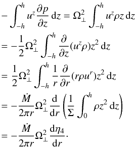
-
(iii)
Energy transport. The structure of the disk has to be such that the actual value of the divergence of the flux corresponds to Eq. (13). Radiative transport is computed in the diffusive approximation
 (14)while convective
transport is computed in a mixing-length approximation. Energy is transported in the
vertical direction through diffusion of radiation or convection according to the
value of the thermodynamical gradient, which can be either radiative or convective.
Accordingly, we take
(14)while convective
transport is computed in a mixing-length approximation. Energy is transported in the
vertical direction through diffusion of radiation or convection according to the
value of the thermodynamical gradient, which can be either radiative or convective.
Accordingly, we take 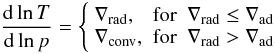 (15)with
the adiabatic gradient given by a derivative at constant entropy:
∇ad ≡ (∂lnT/∂lnp)S.
The radiative gradient ∇rad is calculated in the diffusive approximation,
(15)with
the adiabatic gradient given by a derivative at constant entropy:
∇ad ≡ (∂lnT/∂lnp)S.
The radiative gradient ∇rad is calculated in the diffusive approximation,
 (16)where
κR is the Rosseland mean opacity, and
σ is the Stefan-Boltzmann constant. At the equatorial plane we
apply the boundary conditions described in point (iv) below. When the temperature
gradient exceeds the value of the adiabatic gradient, we have to consider the
convective energy flux. The convective gradient ∇conv is calculated using
the mixing length theory introduced by Paczyński
(1969). We take the following mixing length,
(16)where
κR is the Rosseland mean opacity, and
σ is the Stefan-Boltzmann constant. At the equatorial plane we
apply the boundary conditions described in point (iv) below. When the temperature
gradient exceeds the value of the adiabatic gradient, we have to consider the
convective energy flux. The convective gradient ∇conv is calculated using
the mixing length theory introduced by Paczyński
(1969). We take the following mixing length, 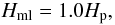 (17)with
pressure scale height Hp defined as (Hameury et al. 1998)
(17)with
pressure scale height Hp defined as (Hameury et al. 1998) 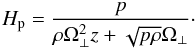 (18)The convective
gradient is defined by the formula
(18)The convective
gradient is defined by the formula  (19)where
y is the solution of the equation
(19)where
y is the solution of the equation 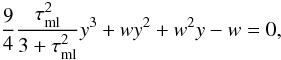 (20)with the typical
optical depth for convection
τml = ρκRHml,
and w given by
(20)with the typical
optical depth for convection
τml = ρκRHml,
and w given by 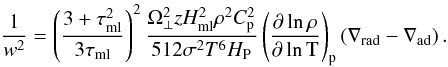 (21)The thermodynamical
quantities Cp, ∇ad and
(∂lnρ/∂lnT)p
are calculated using standard formulae (e.g., Chandrasekhar 1967) assuming solar abundances (X = 0.70,
Y = 0.28) and, when necessary, taking the effect of partial
ionization of gas on the gas mean molecular weight into account . We use Rosseland
mean opacities κR (including the
processes of absorption and scattering) taken from Alexander et al. (1983) and Seaton et al.
(1994). Following other authors (e.g., Idan
et al. 2008), we neglect expansion opacities, in agreement with our neglect
of vertical velocity gradients.
(21)The thermodynamical
quantities Cp, ∇ad and
(∂lnρ/∂lnT)p
are calculated using standard formulae (e.g., Chandrasekhar 1967) assuming solar abundances (X = 0.70,
Y = 0.28) and, when necessary, taking the effect of partial
ionization of gas on the gas mean molecular weight into account . We use Rosseland
mean opacities κR (including the
processes of absorption and scattering) taken from Alexander et al. (1983) and Seaton et al.
(1994). Following other authors (e.g., Idan
et al. 2008), we neglect expansion opacities, in agreement with our neglect
of vertical velocity gradients. -
(iv)
We set the following boundary conditions. At the equatorial plane (z = 0) we set ℱ(0) = 0, in accordance with the assumption of reflection symmetry, while at the disk surface, τ(h) = 0, we follow the Eddington approximation (Mihalas 1982) and require
 . In practice, for a fixed
r, and prescribed values of Tc and
fadv, a trial value of the central density,
ρc, is assumed and the equations are integrated in
z until
ρ(z∗) = 10-16gcm-3
(as a stand-in for the disk surface,
z∗ = h). If ℱ(h)
and T(h) fail to satisfy the surface boundary
condition, the assumed value of ρc is adjusted, and the
integration is repeated, until the condition
ℱ(h) = 2σT4(h)
is met. Convergence is usually attained in a few iterations. The emergent flux of
radiation at any given r is then
F = ℱ(h).
. In practice, for a fixed
r, and prescribed values of Tc and
fadv, a trial value of the central density,
ρc, is assumed and the equations are integrated in
z until
ρ(z∗) = 10-16gcm-3
(as a stand-in for the disk surface,
z∗ = h). If ℱ(h)
and T(h) fail to satisfy the surface boundary
condition, the assumed value of ρc is adjusted, and the
integration is repeated, until the condition
ℱ(h) = 2σT4(h)
is met. Convergence is usually attained in a few iterations. The emergent flux of
radiation at any given r is then
F = ℱ(h).
2.3. Radial structure equations
The radial sector of the model is described by four laws of conservation and a regularity condition:
-
(i)
Mass conservation,
 (22)
(22) -
(ii)
Conservation of angular momentum,
 (23)where
ℒ = uφ is the specific angular
momentum, ℒin is a constant, whose value is to be specified later, and Γ
is the Lorentz factor (Gammie & Popham
1998):
(23)where
ℒ = uφ is the specific angular
momentum, ℒin is a constant, whose value is to be specified later, and Γ
is the Lorentz factor (Gammie & Popham
1998): 
-
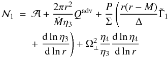
(iii)
Conservation of radial momentum,
 (24)where
  (25)and
Ω = uφ/ut
is the angular velocity with respect to a stationary observer,
(25)and
Ω = uφ/ut
is the angular velocity with respect to a stationary observer,
 is the angular velocity with respect to
an inertial observer,
is the angular velocity with respect to
an inertial observer,  are the angular
frequencies of the corotating and counterrotating Keplerian orbits and
are the angular
frequencies of the corotating and counterrotating Keplerian orbits and
 is the radius of
gyration. The value of P is taken from vertical structure solutions
for given values of Σ and Tc,
is the radius of
gyration. The value of P is taken from vertical structure solutions
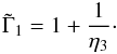
for given values of Σ and Tc,  (26)hence, the
radial derivative of the height-integrated pressure takes the form
(26)hence, the
radial derivative of the height-integrated pressure takes the form 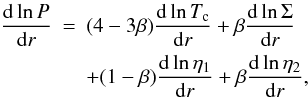 (27)with
β = η2(k/μmp)ΣTc/P.
(27)with
β = η2(k/μmp)ΣTc/P.
-
(iv)
Energy conservation. The advective cooling is defined following Kato et al. (2008) in terms of the vertically integrated quantities, as
 (28)Using mass
conservation (Eq. (22)) and
hydrostatic equilibrium (Eq. (12)),
the expression can be rewritten as
(28)Using mass
conservation (Eq. (22)) and
hydrostatic equilibrium (Eq. (12)),
the expression can be rewritten as  (29)Just
like P, the advective cooling term,
Qadv, and the coefficients
η3, η4 are all determined
from the vertical structure solutions. The manipulation of the last term in
Eq. (28) was as follows:
(29)Just
like P, the advective cooling term,
Qadv, and the coefficients
η3, η4 are all determined
from the vertical structure solutions. The manipulation of the last term in
Eq. (28) was as follows:
3. Numerical method
3.1. Vertical structure
The set of ordinary differential equations describing the vertical structure, i.e., Eqs. (12), (13) and (15) together with appropriate boundary conditions are solved for a given BH spin on a three-dimensional grid spanned by the radius r, the central temperature Tc, and the advection factor fadv. For a given set of these parameters, we start the integration from the equatorial plane (z = 0), and the solution satisfying the outer boundary condition is found as described at the end of Sect. 2.2. The resulting quantities describing the vertical structure (Tc, Σ, Qadv, P, η1, η2, η3, and η4), together with r, are printed out to tables for subsequent use in interpolation routines. As it turns out, the first two of these parameters, Tc and Σ, can be used to uniquely determine all the other quantities characterizing the vertical structure, including fadv (see Fig. 2).
Calculating the full grid of vertical solutions for a single value of BH spin takes about 5 h on a 4-CPU workstation.
3.2. Radial structure
By a series of algebraic manipulations of Eqs. (22)–(24), and (29), we obtain the following set of two
ordinary differential equations for V(r) and
Tc(r) 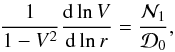 (30)
(30) (31)with
 and
and  given by
 (32)
(32) (33)Typically,
 vanishes close to the black hole, as
ℒ approaches ℒin.
vanishes close to the black hole, as
ℒ approaches ℒin.
To obtain a solution one has to solve this system of two ordinary differential equations,
together with the following regularity conditions at the sonic radius
rS, defined by the same conditions:  (34)as well as outer
boundary conditions given at some large radius rout. The
solution between the outer boundary and the sonic point is found using the relaxation
technique (Press 2002), with ℒin treated
as the eigenvalue of the problem. The sonic point for a∗ = 0
is located at 5.9M for accretion rate
0.01ṀEdd and at 5.0M for
2.0ṀEdd. To start the relaxation process we have to provide
a trial solution that is obtained by a method similar to the one described in Sądowski (2009) assuming the Novikov & Thorne (1973) outer boundary conditions. Once the
trial solution is found, one can start the relaxation process with a free inner boundary
corresponding to the location of the sonic point. To find the solution inside the sonic
point we make a small step inward to cross the critical point and then integrate down to
BH horizon using a Runge-Kutta method of the fourth order. In this work we use 25 mesh
points spaced logarithmically in the radius on the section between the sonic point and
rout = 1000M. This particular number of
grid points is enough to resolve all disk features. We have verified that the results are
accurately reproduced with a denser grid.
(34)as well as outer
boundary conditions given at some large radius rout. The
solution between the outer boundary and the sonic point is found using the relaxation
technique (Press 2002), with ℒin treated
as the eigenvalue of the problem. The sonic point for a∗ = 0
is located at 5.9M for accretion rate
0.01ṀEdd and at 5.0M for
2.0ṀEdd. To start the relaxation process we have to provide
a trial solution that is obtained by a method similar to the one described in Sądowski (2009) assuming the Novikov & Thorne (1973) outer boundary conditions. Once the
trial solution is found, one can start the relaxation process with a free inner boundary
corresponding to the location of the sonic point. To find the solution inside the sonic
point we make a small step inward to cross the critical point and then integrate down to
BH horizon using a Runge-Kutta method of the fourth order. In this work we use 25 mesh
points spaced logarithmically in the radius on the section between the sonic point and
rout = 1000M. This particular number of
grid points is enough to resolve all disk features. We have verified that the results are
accurately reproduced with a denser grid.
The parameters linked to the vertical structure (P, Qadv, η1, η2, η3, and η4) for given Σ and Tc are linearly interpolated from pre-calculated tables of the vertical structure solutions (for any value of V, Σ is determined directly from mass conservation, Eqs. (4), (22)). The radial derivatives dlnη1/dlnr, dlnη2/dlnr, dlnη3/dlnr, and dlnη4/dlnr are evaluated numerically from the η1, η2, η3, and η4 profiles in the previous iteration step. A relaxed solution is obtained in a few iteration steps. Once a solution outside the sonic point is found we numerically estimate the radial derivatives of V and Tc at the sonic point using values given at r > rS and use these derivatives to start direct integration inside the sonic point.
The solution thus obtained may then be used as a trial solution when looking for the relaxation solution of another slim disk, i.e., when one of the three fundamental parameters (Ṁ, a, M) has a slightly different value. Each relaxation step takes approximately 5 seconds on a single-CPU workstation.
4. Results
In the following two sections we present and discuss both the radial and vertical structure of slim accretion disks. All the solutions, if not stated otherwise, were computed assuming α = 0.01 and M = 10 M⊙.
4.1. Disk radial structure
 |
Fig.1 Angular momentum (uφ) in a Schwarzschild slim disk for two accretion rates. For very low accretion rates the angular momentum follows the Keplerian profile (dotted line) down to the ISCO. For high accretion rates the flow is super-Keplerian between the “center” of the disk at rcen and the “potential spout” at rpot. The vertical dot-dashed line on this and subsequent figures denotes the location of the ISCO. |
Angular momentum
The angular momentum profiles for our accretion disk solutions near a nonrotating BH are presented in Fig. 1. Results for two values of mass accretion rate are shown, Ṁ = 0.1MEdd and 2.0MEdd, where ṀEdd = 16LEdd/c2 is the critical accretion rate that for a disk around a nonrotating BH approximately corresponds to the Eddington luminosity, LEdd. For the lowest accretion rates the profiles follow the Keplerian profile and reach its minimal value (ℒin in Eq. (23)) at the marginally stable orbit (ISCO, Bardeen et al. 1972). The higher the accretion rate, the stronger the deviation from the Keplerian profile. The disk is sub-Keplerian at large distances and super-Keplerian at moderate radii. The Keplerian profile is crossed again at a point located inside the marginally stable orbit, and corresponding to what is usually called “the cusp” or “the potential spout”. For a detailed study of the physics of the inner edge of a see Abramowicz et al. (2010).
S-curves
Figure 2 presents slim disk solutions at r = 20M on the Tc-Σ plane, for a nonrotating BH. Solutions of the polytropic, height-averaged models are presented for comparison; for detailed discussion see Sect. 5. The locus of solutions for various values of the mass accretion rate has the shape of the so-called “S-curve” (Abramowicz et al. 1988). The lower, gas-pressure dominated branch accurately follows the track of radiatively efficient solutions (fadv = 0). The middle, radiation-pressure dominated branch is reached at Ṁ ≈ 0.1ṀEdd. As advection becomes significant, the slim-disk solution leaves the fadv = 0 track and moves to higher advection rates (S-curve). Around Ṁ = 5ṀEdd, the solutions enter the upper advection-dominated branch corresponding to fadv > 1.0 (more than 50% of heat stored in the accreted gas). At Ṁ = 20ṀEdd this rate almost increases up to 80% (fadv ≈ 4.0).
 |
Fig.2 The Tc-Σ plane at r = 20M for a nonrotating BH (a∗ = 0). The dotted lines connect solutions for the vertical structure of slim disks that have the same value of the advection parameter fadv. The locus of standard (radiatively efficient, fadv = 0) disk solutions is shown with the thick dotted line. The solid thick line represents the vertical slim-disk solutions for different accretion rates (indicated by triangles), and the dashed line presents corresponding solutions of the conventional polytropic slim-disk model (see Sect. 5). The difference between the two lines in the low Ṁ limit corresponds to the difference in Σ between the two models (see Fig. 17). |
Surface density
Profiles of the surface density for 2-D slim-disk solutions for a non-rotating BH are presented in the upper panel of Fig. 3. Different regimes, corresponding to different branches of the “S-curve” on the (Σ, Tc) plane are visible. For large radii the surface density increases with increasing accretion rate (the lower gas-pressure dominated branch), while this relation is opposite for moderate radii (the middle radiation-pressure dominated branch). For accretion rates Ṁ > 5.0ṀEdd the upper advection-dominated branch would be reached. The local maxima in the surface density profiles (discussed in detail in, e.g., Sądowski 2009) are visible for moderate accretion rates (~0.5 ṀEdd). The bottom panel of Fig. 3 presents corresponding profiles of the radial velocity V as measured by an observer corotating with the fluid.
The surface density dependence on BH rotation is presented in Fig. 4. The profiles are shifted to lower radii as the inner edge of the disk moves inward for higher BH spins. The outer parts of the accretion disk are insensitive to the metric.
 |
Fig.3 Profiles of the surface density (upper panel) and corresponding values of radial velocity V (bottom panel) of a slim disk for a nonrotating BH. Solutions for different accretion rates are presented. |
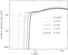 |
Fig.4 Profiles of the surface density for slim disks at a constant accretion rate (Ṁ = 0.1ṀEdd) and various BH spins. |
Optical depth
In the top panel of Fig. 5 we plot the total optical depth of the vertical slim disk solutions for different accretion rates (a∗ = 0). The total optical depth
 where the total opacity
coefficient κR, which includes the processes of absorption and
scattering, is closely related to the surface density. Indeed, the radial profiles of the
optical depth shown in Fig. 5 follow the
corresponding profiles of surface density. Any differences in the profiles come from the
dependence of the opacity coefficient on local density and temperature. Outside the ISCO
the total optical depth is always large
(τtot > 103).
where the total opacity
coefficient κR, which includes the processes of absorption and
scattering, is closely related to the surface density. Indeed, the radial profiles of the
optical depth shown in Fig. 5 follow the
corresponding profiles of surface density. Any differences in the profiles come from the
dependence of the opacity coefficient on local density and temperature. Outside the ISCO
the total optical depth is always large
(τtot > 103).
 |
Fig.5 Optical depth for α = 0.01 slim disks around a Schwarzschild black hole at different accretion rates. Top panel: the total optical depth as a function of the radius. Bottom panel: the effective optical depth as a function of the radius. The ISCO is shown at r = 6M. The shaded region in the bottom plot indicates the region where the diffusive approximation is invalid. |
The diffusive approximation for radiative transport may only be used if photons are absorbed, otherwise LTE cannot be established. In a scattering-dominated atmosphere, the effective optical depth is then the relevant quantity to be used in checking for the self-consistency of the diffusive approximation. The bottom panel of Fig. 5 presents corresponding profiles of the effective optical depth, which is estimated in the following way:
 where
κes = 0.34 cm2g-1 is the mean
opacity for Thomson electron scattering. For
Ṁ > 0.3ṀEdd the inner region of the
disk becomes radiation-pressure dominated (it enters the middle branch on the
corresponding S-curve), the surface density decreases with increasing accretion rate, and
electron scattering begins to dominate absorption. Therefore, the effective optical depth
decreases with increasing accretion rate and reaches values
τeff < 1 in the inner parts of the disk for accretion
rates above 1.0ṀEdd. As a result, for
Ṁ > 1.0ṀEdd, the diffusive
approximation can no longer be applied, and our present approach to solving for the disk
structure breaks down. In Fig. 6 we exhibit the
dependence of the effective optical depth on the value of α. In general,
τeff is inversely proportional to α (as is
the surface density). At lower accretion rates
(Ṁ < 0.1ṀEdd) the effective optical
depth remains large even for high values of α.
where
κes = 0.34 cm2g-1 is the mean
opacity for Thomson electron scattering. For
Ṁ > 0.3ṀEdd the inner region of the
disk becomes radiation-pressure dominated (it enters the middle branch on the
corresponding S-curve), the surface density decreases with increasing accretion rate, and
electron scattering begins to dominate absorption. Therefore, the effective optical depth
decreases with increasing accretion rate and reaches values
τeff < 1 in the inner parts of the disk for accretion
rates above 1.0ṀEdd. As a result, for
Ṁ > 1.0ṀEdd, the diffusive
approximation can no longer be applied, and our present approach to solving for the disk
structure breaks down. In Fig. 6 we exhibit the
dependence of the effective optical depth on the value of α. In general,
τeff is inversely proportional to α (as is
the surface density). At lower accretion rates
(Ṁ < 0.1ṀEdd) the effective optical
depth remains large even for high values of α.
 |
Fig.6 Profiles of the effective optical depth of a Schwarzschild slim disk for three values of viscosity (α = 0.01, 0.05, and 0.1), calculated for two accretion rates, 0.1ṀEdd (dashed lines) and 1.0ṀEdd (solid lines). |
Flux profiles
Profiles of the flux emitted from the disk surface ( ) in the
case of a nonrotating BH are presented in Fig. 7.
Results corresponding to accretion rates from 0.01 up to
5.0ṀEdd are shown. For the lowest rates the emission from
inside the marginally stable orbit is negligible as expected in the standard accretion
disk models. This is no longer true for higher accretion rates, and the advection of
energy causes significant emission from smaller radii (Abramowicz et al. 2010). For super-Eddington accretion rates the emitted flux
continues to grow with a decreasing radius even inside the marginally stable orbit.
Radiation coming from the direct vicinity of the black hole is suppressed by the
gravitational redshift (the g-factor). Therefore, an observer at infinity
will observe a maximum in the profile of the effective temperature even for the highest
accretion rates.
) in the
case of a nonrotating BH are presented in Fig. 7.
Results corresponding to accretion rates from 0.01 up to
5.0ṀEdd are shown. For the lowest rates the emission from
inside the marginally stable orbit is negligible as expected in the standard accretion
disk models. This is no longer true for higher accretion rates, and the advection of
energy causes significant emission from smaller radii (Abramowicz et al. 2010). For super-Eddington accretion rates the emitted flux
continues to grow with a decreasing radius even inside the marginally stable orbit.
Radiation coming from the direct vicinity of the black hole is suppressed by the
gravitational redshift (the g-factor). Therefore, an observer at infinity
will observe a maximum in the profile of the effective temperature even for the highest
accretion rates.
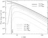 |
Fig.7 Flux emitted from the surface of a slim disk at five accretion rates onto a Schwarzschild black hole. At high accretion rates significant emmision from within the ISCO is clearly visible in the figure. |
The increase in the advective flux with increasing accretion rate is clearly visible in Fig. 8. The ratio of the heat advected to the amount of energy emitted is presented for different accretion rates. For very low accretion rates these profiles approach the limit of a radiatively efficient disk (fadv ≡ 0), and the advection component becomes significant for higher accretion rates. Some part (up to 30% at r = 20M for 2.0ṀEdd) of the energy generated at moderate radii is advected with matter and radiated away at r < 10M. This causes the significant change in the emitted flux profile at the higher accretion rates visible in Fig. 7.
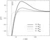 |
Fig.8 Profiles of the advection coefficient fadv for different accretion rates (Schwarzschild black hole). |
In Fig. 9 we present the emitted flux profiles for different BH angular momenta at a constant accretion rate Ṁ = 0.1ṀEdd. These profiles coincide at large radii where the influence of the BH rotation is negligible; however, the higher the BH spin, the closer to the horizon the marginally stable orbit. Therefore, in the case of rotating BHs, the accreting matter can move much deeper into the gravity well, compared to nonrotating BHs. This effect leads to an increase in the disk luminosity and hardening of its spectrum, which can be inferred from Fig. 9 – the higher the spin, the higher the disk luminosity, and the higher the flux (which corresponds to the effective temperature).
 |
Fig.9 Flux profiles at fixed accretion rate (Ṁ = 0.1ṀEdd) for five values of BH spin. |
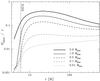 |
Fig.10 The height of the photosphere at different accretion rates onto a Schwarzschild black hole. |
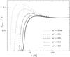 |
Fig.11 Profiles of photospheric height at a constant accretion rate (Ṁ = 0.1ṀEdd) and various BH spins. |
Photosphere location
The flux observed at infinity may be obtained by performing ray tracing of photons emitted from the accretion disk (see Sect. 5). Scattering in the layer above the photosphere must also be taken into account. An accurate calculation requires detailed knowledge of atmospheric properties, including the location of the photosphere. This is particularly important when accretion rates are high and the disk is no longer geometrically thin (Sądowski et al. 2009).
In Fig. 10 we plot the profiles for the
z-location of the photosphere, Hphot,
obtained in our model at different accretion rates for a nonrotating black hole. Clearly,
for high accretion rates, Ṁ > 0.1ṀEdd,
the inner regions become thicker (effects of radiation pressure). For
Ṁ = 1.0ṀEdd, the ratio
Hphot/r reaches a value as high as 0.25.
Close to the ISCO the height of the photosphere rapidly decreases because of vigorous
cooling (compare Fig. 8). Although the rapid change
in disk thickness violates the assumption of the hydrostatic equilibrium that we make when
solving for the disk vertical structure, the accelerations connected with the vertical
motions involved are much lower than the vertical component of gravity. Indeed, the
vertical accelerations are close to  . In deriving this
estimate we liberally assumed that dH/dr ~ 1
and used the fact that the rapid decrease in disk height occurs near the sonic point,
while the speed of sound vs is approximately
rΩ ⊥ (H/r). Thus the
acceleration terms modifying Eq. (12) would
be smaller than the gravitational acceleration by a factor of a few percent:
(H/r) ~ 10-1. In Fig. 12 we plot the dynamical and gravitational components of
the vertical equilibrium equation at the photosphere. It is clear that the former is at
least 10 times smaller than the latter at the sonic radii for
Ṁ ≤ ṀEdd. Therefore, in all likelihood, our
results correctly describe the disk structure that would be obtained without assuming
strict hydrostatic equilibrium.
. In deriving this
estimate we liberally assumed that dH/dr ~ 1
and used the fact that the rapid decrease in disk height occurs near the sonic point,
while the speed of sound vs is approximately
rΩ ⊥ (H/r). Thus the
acceleration terms modifying Eq. (12) would
be smaller than the gravitational acceleration by a factor of a few percent:
(H/r) ~ 10-1. In Fig. 12 we plot the dynamical and gravitational components of
the vertical equilibrium equation at the photosphere. It is clear that the former is at
least 10 times smaller than the latter at the sonic radii for
Ṁ ≤ ṀEdd. Therefore, in all likelihood, our
results correctly describe the disk structure that would be obtained without assuming
strict hydrostatic equilibrium.
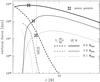 |
Fig.12 Comparison of the dynamical
(vrdvz/dr ≈ Vd(VdH/dr)/dr)
and gravitational ( |

In Fig. 11 we present radial photosphere profiles, at a fixed accretion rate and different values of the BH spin. The photospheric heights coincide for large radii. In the inner regions of the disk, the height of the photosphere increases with BH spin, reflecting the increased luminosity and radiation pressure.
4.2. Vertical structure
In Fig. 13 we present a vertical cross-section of a Schwarzschild slim disk for Ṁ = 0.01ṀEdd. At this accretion rate the disk is radiatively efficient and no advection of entropy is expected. The top panel presents the radial profiles of the photosphere and the disk surface (defined as a layer with ρ = 10-16g/cm3).
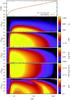 |
Fig.13 Vertical structure of a slim disk for Ṁ = 0.01ṀEdd and a∗ = 0. The top panel presents the surface of the disk (green dashed line), and the photospheric surface (red solid line). The other panels present the structure of the disk below the photosphere. Top to bottom: total optical thickness, temperature, density, vertical flux of energy, and the termodynamical gradient. The blue solid line in the bottom panel delimits the convective region. |
The total optical depth reaches values as high as ~20000 on the equatorial plane and decreases monotonically towards the photosphere at τ = 2/3 (Fig. 13, second panel from the top). Within the marginally stable orbit, the total optical depth significantly decreases, as shown in Fig. 5.
The third panel of Fig. 13 presents the temperature, which decreases with height from Tc at the equatorial plane to Teff at the photosphere. The maximum value of the temperature is attained on the equatorial plane at r ~ 10M.
Density is presented in the fourth panel, and the next panel presents the vertical flux that is generated inside the disk according to Eq. (13). It is set to zero on the equatorial plane by reflection symmetry, and then rapidly increases, because in an alpha disk the dissipation is proportional to the pressure, which reaches its maximum on the z = 0 plane. Close to the disk surface, where pressure is almost negligible, the flux slowly settles down to the emitted value. At the accretion rate chosen for the figure the flux rapidly decreases inside the marginally stable orbit.
The bottom panel of Fig. 13 presents the nonmonotonic distribution of the termodynamical gradient (Eq. (15)), which ranges between 0.2 and 0.4. Therefore, the disk’s vertical structure cannot be described by a simple polytropic relation. Moreover, in the region of the highest temperature (close to the equatorial plane at moderate radii, r ≈ 20M), the heat is transported upward through convection.
The vertical structure of an accretion disk with ten times higher accretion rate, Ṁ = 0.1ṀEdd, is presented in Fig. 14. The general picture remains the same, since the advection of heat is still insignificant. However, as the temperatures increase, the inner disk regions become dominated by radiation pressure. For 0.1ṀEdd the convective region extends from the marginally stable orbit up to 300M and covers more than half of the disk thickness.
The disk structure is significantly different in the case of a high accretion rate (e.g., 1.0ṀEdd), with a significant amount of advection. The vertical cross-sections of the slim disk are presented in Fig. 15. The inner regions are dominated by radiation pressure, so the disk geometrically thickens and the photosphere is now higher. The total optical depth mostly follows the surface density (compare Fig. 5), and therefore decreases considerably towards the black hole in the inner parts of the disk.
The temperature maximum is again located at the equatorial plane close to r ≈ 10M. The maximum of the effective temperature (corresponding to the vertical flux shown in the fifth panel (compare also Fig. 7) is shifted inwards, down to r ≈ 8M.
The fourth panel of Fig. 15 presents the density distribution. Despite the fact that the surface density monotonically increases outwards (see Fig. 3), ρ has two maxima in the equatorial plane: at r ≈ 200M and r ≈ 6M. Finally, the bottom panel presents the termodynamical gradient distribution. For such a high accretion rate, the convective zone extends nearly to the photosphere for r < 200M and is present up to r = 2000M.
 |
Fig.16 Meridional profiles of density for three accretion rates: Ṁ = 0.01 (top), 0.1 (middle) and 1.0ṀEdd (bottom panel) in (r,z) coordinates. The violet boundaries show the location of the photosphere. The black hole is described by MBH = 10M⊙, and a∗ = 0. |
In Fig. 16 we present the density in the meridional plane for three different accretion rates. The equatorial plane lies in the middle of each plot. The violet boundaries denote the photosphere. The two maxima of density at the equatorial plane for Ṁ = 1.0ṀEdd) are clearly visible also in this representation, as are some other features discussed above.
5. Comparison with height-averaged slim disk solutions
In this section we compare our 2-D slim disk solutions, where the radial structure equations are coupled to those for the vertical structure, with the standard polytropic slim disk model, in which the slim-disk equations and properties are averaged over the thickness of the disk (e.g., Kato et al. 2008). We note here that the slim disk solutions presented in one of our previous papers (Sądowski 2009) did not follow the polytropic formalism, assuming different relations between the vertically integrated quantities and their values on the equatorial plane (e.g., Σ = 2ρ0H instead of Σ = 2INρ0H, where IN is defined in Eq. (37)) In this work, we also use a more general form of the energy equation (compare our Eq. (29) with Eq. (6) in Sądowski 2009).
Let us assume the polytropic equation of state with the polytropic index
N:
p = Kρ1 + 1/N.
The vertical integration of the hydrostatic equilibrium formula, Eq. (12), gives  (35)We also assume
 (36)One can now calculate
analytical formulae for η1 to η4
(Sect. 2.3):
(36)One can now calculate
analytical formulae for η1 to η4
(Sect. 2.3):
 where
where
 (37)
(37) (38)In this approach we
do not solve the vertical structure consistently, so we need to make some additional
assumptions about the vertical equilibrium of forces and radiation transfer. Following other
authors, we simplify the hydrostatic equilibrium (Eq. (12)) by applying a finite difference approximation and write
(38)In this approach we
do not solve the vertical structure consistently, so we need to make some additional
assumptions about the vertical equilibrium of forces and radiation transfer. Following other
authors, we simplify the hydrostatic equilibrium (Eq. (12)) by applying a finite difference approximation and write
 (39)One has to remember that
disk thickness, H, defined in this way is not the exact location of the
photosphere. Therefore we introduce a factor fH
relating these quantities,
(39)One has to remember that
disk thickness, H, defined in this way is not the exact location of the
photosphere. Therefore we introduce a factor fH
relating these quantities,  (40)Assuming that radiation
is transported in the vertical direction through diffusion, the radiative flux is given by
(40)Assuming that radiation
is transported in the vertical direction through diffusion, the radiative flux is given by
 (41)Under the one-zone
approximation one obtains the following formula for the total flux emitted from disk
surface,
(41)Under the one-zone
approximation one obtains the following formula for the total flux emitted from disk
surface,
 |
Fig.17 Comparison of the flux, disk thickness (the height of the photosphere for models presented in this paper and of the zero-density surface for 1-D polytropic models) and surface density profiles calculated using the 2-D (this paper, solid lines) and the usual polytropic (N = 3, dotted lines) slim disk models for α = 0.1. The solutions for two accretion rates (0.1 and 1.0ṀEdd) are presented with thick and thin lines, respectively. |
 (42)where factor
fF has been introduced to account for
inaccuracies arising from this approximation, as well as from the dominance of the disk
convection in certain regions (as discussed in Sect. 4.2). Now, advective cooling takes the form
(42)where factor
fF has been introduced to account for
inaccuracies arising from this approximation, as well as from the dominance of the disk
convection in certain regions (as discussed in Sect. 4.2). Now, advective cooling takes the form
 (43)Usually, the following
values of N, fH and
fF are assumed:
(43)Usually, the following
values of N, fH and
fF are assumed:  (44)In
Fig. 17 we compare radial profiles of the flux,
photospheric height and surface density of the 2-D slim disk model described in this paper
(consistently taking its vertical structure into account) with profiles obtained for the
polytropic, height-averaged, slim disk, as presented in this section with parameters defined
in Eq. (44). The comparison was carried out
for two accretion rates (0.1 and 1.0ṀEdd), with
α = 0.01. For the lower accretion rate
(0.1ṀEdd), the disk is radiatively efficient (advective
cooling is negligible), and therefore both flux profiles almost coincide and correspond to
the Novikov & Thorne solutions. However, the disk photosphere location in the
polytropic model turns out to be overestimated by more than 20% in the region corresponding
to the maximal emission. The profiles of the surface density do not coincide either, the 2-D
solutions giving values ~25% lower than the corresponding polytropic solutions
(compare Fig. 2).
(44)In
Fig. 17 we compare radial profiles of the flux,
photospheric height and surface density of the 2-D slim disk model described in this paper
(consistently taking its vertical structure into account) with profiles obtained for the
polytropic, height-averaged, slim disk, as presented in this section with parameters defined
in Eq. (44). The comparison was carried out
for two accretion rates (0.1 and 1.0ṀEdd), with
α = 0.01. For the lower accretion rate
(0.1ṀEdd), the disk is radiatively efficient (advective
cooling is negligible), and therefore both flux profiles almost coincide and correspond to
the Novikov & Thorne solutions. However, the disk photosphere location in the
polytropic model turns out to be overestimated by more than 20% in the region corresponding
to the maximal emission. The profiles of the surface density do not coincide either, the 2-D
solutions giving values ~25% lower than the corresponding polytropic solutions
(compare Fig. 2).
For the higher accretion rate (1.0ṀEdd), the flux profiles remain similar (up to 1%). However, as advection becomes important, the emission is shifted inwards with respect to the Novikov & Thorne profile. The photosphere location in the polytropic model is overestimated by ~30% and the surface density by ~20%.
A question arises as to whether such differences in the flux, photosphere, and surface density profiles affect the resulting disk spectrum. In Fig. 18 we present spectral profiles and their ratios (2-D to polytropic) for two accretion rates. The spectra were calculated with ray-tracing routines (Bursa 2006) using the BHSPEC package (Davis et al. 2005), assuming the inclination angle i = 70° and distance to the observer d = 10kpc. As BHSPEC gives tabulated solutions of the full, frequency-dependent, radiative transfer equations for the disk vertical structure taking the Compton scatterings into account in the disk atmosphere, the spectra presented in Fig. 18 are not those of a simple multi-color blackbody. However, one should be aware that using BHSPEC for calculating spectral color correction is not consistent with the assumed vertical structure (calculated or height-averaged) because it is based on a stand-alone disk model.
 |
Fig.18 The upper panel presents spectral profiles of the 2-D and polytropic solutions for two accretion rates (0.1 and 1.0ṀEdd), at inclination angle i = 70o and distance d = 10kpc. The bottom panel presents ratios of the corresponding spectra (of 2-D to polytropic solutions) for both accretion rates. |
The general shape of the spectra is similar for both types of slim disk models, because the emission profiles nearly coincide. However, the spectra are not identical. The bottom panel of Fig. 18 presents ratios of the spectral profiles of the corresponding solutions for each accretion rate. They all coincide att low energies (<0.1keV), while for higher energies the discrepancies are as large as 3% for 1.0ṀEdd at 5 keV. These differences are atributed to (slightly) different profiles of the flux, the photosphere, and the surface density. We conclude that the proper treatment of the vertical structure hardly affects the spectra of slim disks for this range of accretion rates (Ṁ < ṀEdd) and the viscosity parameter (α ≤ 0.01).
We end this section by giving fitting formulae for N,
fH, and
fF, which approximate the full numerical
2-D solutions described in this paper with a polytropic slim disk model. An advantage of
using these formulae lies in avoiding the need to perform time-consuming calculations of the
vertical structure and avoiding numerical problems connected to interpolation in the
vertical solutions grid. The formulae for the polytropic model parameters for
α = 0.01 are 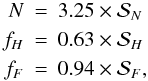 (45)where
the spin correction coefficients
(45)where
the spin correction coefficients  ,
,  , and
, and
 are given by
  Here,
rms is the radius of the marginally stable orbit. For a
nonrotating BH, at the radius r = 7M (corresponding to the
highest disk effective temperature), the fitting formulae are accurate to 1% for the emitted
flux, the photospheric height and the surface density.
Here,
rms is the radius of the marginally stable orbit. For a
nonrotating BH, at the radius r = 7M (corresponding to the
highest disk effective temperature), the fitting formulae are accurate to 1% for the emitted
flux, the photospheric height and the surface density.
6. Discussion
Motivated by a desire to explain and fit the observed spectra of accreting black holes in binary systems to theoretical models, we have developed a 2-D model of optically thick slim disks. These should be particularly relevant to transient binaries. In quiescence, their inner disk regions are described well by optically thin advection-dominated accretion flows (ADAFs; see e.g., Lasota et al. 1996; Dubus et al. 2001). However, a few black hole systems (e.g., GRS 1915+105 and LMC X-3) have been observed in thermal states corresponding to disk luminosities higher than 0.3LEdd (McClintock & Remillard 2003; Steiner et al. 2010), and modeling these require optically thick models going beyond the standard thin disks.
In this work we present a 2-D slim disk model, in which the radial and vertical structures are coupled. Such an approach eliminates arbitrary factors that influence solutions of the usual polytropic slim disk model. The results were obtained under two key assumptions: an alpha disk was assumed (dissipation proportional to pressure), with a uniform value of α, and the fraction of the generated entropy that is advected was computed at every radius under the assumption that this fraction does not vary with the height above the disk plane (Eq. (13)). Both of these assumptions seem arbitrary, and we can offer no physical motivation for the (conventional) choice we made.
Under these assumptions and for the value α = 0.01 of the viscosity parameter, we computed and presented the detailed structure of 2-D slim disks, parametrized by the mass accretion rate, and the two Kerr metric parameters, M and a. Somewhat surprisingly, the spectra observed at infinity from such disks differ by only a few percent from those obtained from previously considered slim disk models (in which the equations and structure correspond to a height average over a polytropic atmosphere). Such differences are unlikely to introduce any large corrections to spin measurements based on X-ray continuum fits made with corresponding height-averaged polytropic models of slim disks. However, already the latter produce significantly softer spectra in the sub-Eddington regime than the Novikov & Thorne model. For high luminosities, fits based on slim disk models may therefore provide higher values of the black hole spin parameter than corresponding fits based on the kerrbb model (e.g., Shafee et al. 2006). This issue will be discussed in detail in a forthcoming paper (Bursa & Sądowski, in prep.).
One has to be aware that the model of vertical structure presented here is only an approximation of the real physical processes taking place in disk interiors. The diffusion approximation and the convection treatment in the mixing length approach are known to successfully describe media with large effective optical depths but break down when the disk becomes optically thin. We have shown that the effective optical depth of slim accretion disks may drop below unity for super-Eddington luminosities and sufficiently high values of α. For such conditions, a more sophisticated model of radiation transfer should be implemented. However, for α ≤ 0.01 and L ≤ LEdd the assumptions of this work are self-consistent. For higher values of α their range of applicability is limited to lower luminosities (e.g., to 0.5LEdd for α = 0.1). Kerr-metric slim disks with low effective optical depth were discussed by Beloborodov (1998), who finds them to be significantly hotter than the optically thick ones. We have already started implementing a radiative transfer scheme valid for disks with small effective optical depths into the scheme introduced in this work. It will be presented and discussed in a future paper.
Another remark is connected to the fact that one can expect winds to be blown out of the disk surface at super-Eddington luminosities. Such a phenomenon may significantly change the disk structure, e.g., its thickness. This feature of slim disks, not described in our calculations, has recently been cleverly modeled by Dotan & Shaviv (2010).
Acknowledgments
This work was supported in part by Polish Ministry of Science grants N203 0093/1466, N203 304035, N203 380336, N N203 381436. J.P.L. acknowledges support from the French Space Agency CNES, MB from ESA PECS project No. 98040. We thank the anonymous referee for valuable comments.
References
- Abramowicz, M. A., Czerny, B., Lasota, J. P., & Szuszkiewicz, E. 1988, ApJ, 332, 646 [NASA ADS] [CrossRef] [Google Scholar]
- Abramowicz, M. A., Chen, X.-M., Granath, M., & Lasota, J.-P. 1996, ApJ, 471, 762 [NASA ADS] [CrossRef] [Google Scholar]
- Abramowicz, M. A., Lanza, A., & Percival, M. J. 1997, ApJ, 479, 179 [NASA ADS] [CrossRef] [Google Scholar]
- Abramowicz, M. A., Jaroszynski, M., Kato, S., et al. 2010, A&A, 521, A15 [NASA ADS] [CrossRef] [EDP Sciences] [Google Scholar]
- Alexander, D. R., Rypma, R. L., & Johnson, H. R. 1983, ApJ, 272, 773 [NASA ADS] [CrossRef] [Google Scholar]
- Bardeen, J. M., Press, W. H., & Teukolsky, S. A. 1972, ApJ, 178, 347 [NASA ADS] [CrossRef] [Google Scholar]
- Beloborodov, A. M. 1998, MNRAS, 297, 739 [NASA ADS] [CrossRef] [Google Scholar]
- Bursa, M. 2006, PhD Thesis, Charles University, Prague [Google Scholar]
- Chandrasekhar, S. 1967, An introduction to the study of stellar structure (New York: Dover) [Google Scholar]
- Davis, S. W., & Hubeny, I. 2006, ApJS, 164, 530 [NASA ADS] [CrossRef] [Google Scholar]
- Davis, S. W., Blaes, O. M., Hubeny, I., & Turner, N. J. 2005, ApJ, 621, 372 [NASA ADS] [CrossRef] [Google Scholar]
- Dotan, C., & Shaviv, N. J. 2010 [arXiv:1004.1797] [Google Scholar]
- Dubus, G., Hameury, J.-M., & Lasota, J.-P. 2001, A&A, 373, 251 [NASA ADS] [CrossRef] [EDP Sciences] [Google Scholar]
- Gammie, C. F., & Popham, R. 1998, ApJ, 498, 313 [NASA ADS] [CrossRef] [Google Scholar]
- Hameury, J.-M., Menou, K., Dubus, G., Lasota, J.-P., & Hure, J.-M. 1998, MNRAS, 298, 1048 [NASA ADS] [CrossRef] [Google Scholar]
- Hubeny, I. 1991, in Structure and Emission Properties of Accretion Disks, ed. C. Bertout, S. Collin-Souffrin, & J. P. Lasota, Proc. IAU Colloq. 129, 227 [Google Scholar]
- Idan, I., Lasota, J.-P., Hameury, J.-M., & Shaviv, G. 2010, A&A, 519, 117 [Google Scholar]
- Kato, S. 1993, PASJ, 45, 219 [NASA ADS] [Google Scholar]
- Kato, S., Fukue, J., & Mineshige, S. 2008, Black-Hole Accretion Disks — Towards a New Paradigm [Google Scholar]
- King, A. R., Pringle, J. E., & Livio, M. 2007, MNRAS, 376, 1740 [NASA ADS] [CrossRef] [Google Scholar]
- Kluzniak, W., & Kita, D., 2000 [arXiv:astro-ph/0006266] [Google Scholar]
- Lasota, J. P. 1994, in Theory of Accretion Disks - 2, ed. W. J. Duschl, J. Frank, F. Meyer, E. Meyer-Hofmeister, & W. M. Tscharnuter, NATO ASIC Proc. 417, 341 [Google Scholar]
- Lasota, J. P. 2001, New Astron. Rev., 45, 449 [NASA ADS] [CrossRef] [Google Scholar]
- Lasota, J.-P., Narayan, R., & Yi, I. 1996, A&A, 314, 813 [NASA ADS] [Google Scholar]
- McClintock, J. E., & Remillard, R. A. 2003 [arXiv:astro-ph/0306213] [Google Scholar]
- Middleton, M., Done, C., Gierliński, M., & Davis, S. W. 2006, MNRAS, 373, 1004 [NASA ADS] [CrossRef] [Google Scholar]
- Mihalas, D. M. 1982, Stellar atmospheres., ed. D. M. Mihalas [Google Scholar]
- Misner, C. W., Thorne, K. S., & Wheeler, J. A. 1973 (San Francisco: W. H. Freeman and Co.) [Google Scholar]
- Novikov, I. D., & Thorne, K. S. 1973, in Black Holes (Les Astres Occlus), 343 [Google Scholar]
- Paczyński, B. 1969, Acta Astron., 19, 1 [NASA ADS] [Google Scholar]
- Penna, R. F., McKinney, J. C., Narayan, R., et al. 2010, MNRAS, 408, 752 [NASA ADS] [CrossRef] [Google Scholar]
- Press, W. H. 2002, Numerical recipes in C++: the art of scientific computing [Google Scholar]
- Różańska, A., & Madej, J. 2008, MNRAS, 386, 1872 [NASA ADS] [CrossRef] [Google Scholar]
- Sądowski, A. 2009, ApJS, 183, 171 [NASA ADS] [CrossRef] [Google Scholar]
- Sądowski, A., Abramowicz, M. A., Bursa, M., et al. 2009, A&A, 502, 7 [NASA ADS] [CrossRef] [EDP Sciences] [Google Scholar]
- Schreiber, M. R., & Lasota, J.-P. 2007, A&A, 473, 897 [NASA ADS] [CrossRef] [EDP Sciences] [Google Scholar]
- Seaton, M. J., Yan, Y., Mihalas, D., & Pradhan, A. K. 1994, MNRAS, 266, 805 [NASA ADS] [CrossRef] [Google Scholar]
- Shafee, R., McClintock, J. E., Narayan, R., et al. 2006, ApJ, 636, L113 [NASA ADS] [CrossRef] [Google Scholar]
- Shakura, N. I., & Sunyaev, R. A. 1973, A&A, 24, 337 [NASA ADS] [Google Scholar]
- Shaviv, G., & Wehrse, R. 1986, A&A, 159, L5 [NASA ADS] [Google Scholar]
- Smak, J. 1999, Acta Astron., 49, 391 [NASA ADS] [Google Scholar]
- Smak, J. 2010, Acta Astron., 60, 83 [NASA ADS] [Google Scholar]
- Steiner, J. F., McClintock, J. E., Narayan, R., Remillard, R. A., & Gou, L. 2010, BAAS, 41, 225 [Google Scholar]
- Urpin, V. A. 1984, Astron. Z., 61, 84 [Google Scholar]
All Figures
|
Fig.1 Angular momentum (uφ) in a Schwarzschild slim disk for two accretion rates. For very low accretion rates the angular momentum follows the Keplerian profile (dotted line) down to the ISCO. For high accretion rates the flow is super-Keplerian between the “center” of the disk at rcen and the “potential spout” at rpot. The vertical dot-dashed line on this and subsequent figures denotes the location of the ISCO. |
| In the text | |
|
Fig.2 The Tc-Σ plane at r = 20M for a nonrotating BH (a∗ = 0). The dotted lines connect solutions for the vertical structure of slim disks that have the same value of the advection parameter fadv. The locus of standard (radiatively efficient, fadv = 0) disk solutions is shown with the thick dotted line. The solid thick line represents the vertical slim-disk solutions for different accretion rates (indicated by triangles), and the dashed line presents corresponding solutions of the conventional polytropic slim-disk model (see Sect. 5). The difference between the two lines in the low Ṁ limit corresponds to the difference in Σ between the two models (see Fig. 17). |
| In the text | |
|
Fig.3 Profiles of the surface density (upper panel) and corresponding values of radial velocity V (bottom panel) of a slim disk for a nonrotating BH. Solutions for different accretion rates are presented. |
| In the text | |
|
Fig.4 Profiles of the surface density for slim disks at a constant accretion rate (Ṁ = 0.1ṀEdd) and various BH spins. |
| In the text | |
|
Fig.5 Optical depth for α = 0.01 slim disks around a Schwarzschild black hole at different accretion rates. Top panel: the total optical depth as a function of the radius. Bottom panel: the effective optical depth as a function of the radius. The ISCO is shown at r = 6M. The shaded region in the bottom plot indicates the region where the diffusive approximation is invalid. |
| In the text | |
|
Fig.6 Profiles of the effective optical depth of a Schwarzschild slim disk for three values of viscosity (α = 0.01, 0.05, and 0.1), calculated for two accretion rates, 0.1ṀEdd (dashed lines) and 1.0ṀEdd (solid lines). |
| In the text | |
|
Fig.7 Flux emitted from the surface of a slim disk at five accretion rates onto a Schwarzschild black hole. At high accretion rates significant emmision from within the ISCO is clearly visible in the figure. |
| In the text | |
|
Fig.8 Profiles of the advection coefficient fadv for different accretion rates (Schwarzschild black hole). |
| In the text | |
|
Fig.9 Flux profiles at fixed accretion rate (Ṁ = 0.1ṀEdd) for five values of BH spin. |
| In the text | |
|
Fig.10 The height of the photosphere at different accretion rates onto a Schwarzschild black hole. |
| In the text | |
|
Fig.11 Profiles of photospheric height at a constant accretion rate (Ṁ = 0.1ṀEdd) and various BH spins. |
| In the text | |
|
Fig.12 Comparison of the dynamical
(vrdvz/dr ≈ Vd(VdH/dr)/dr)
and gravitational ( |
| In the text | |
|
Fig.13 Vertical structure of a slim disk for Ṁ = 0.01ṀEdd and a∗ = 0. The top panel presents the surface of the disk (green dashed line), and the photospheric surface (red solid line). The other panels present the structure of the disk below the photosphere. Top to bottom: total optical thickness, temperature, density, vertical flux of energy, and the termodynamical gradient. The blue solid line in the bottom panel delimits the convective region. |
| In the text | |
 |
Fig.14 Same as Fig. 13 but for Ṁ = 0.1ṀEdd. |
| In the text | |
 |
Fig.15 Same as Fig. 13 but for Ṁ = 1.0ṀEdd. |
| In the text | |
|
Fig.16 Meridional profiles of density for three accretion rates: Ṁ = 0.01 (top), 0.1 (middle) and 1.0ṀEdd (bottom panel) in (r,z) coordinates. The violet boundaries show the location of the photosphere. The black hole is described by MBH = 10M⊙, and a∗ = 0. |
| In the text | |
|
Fig.17 Comparison of the flux, disk thickness (the height of the photosphere for models presented in this paper and of the zero-density surface for 1-D polytropic models) and surface density profiles calculated using the 2-D (this paper, solid lines) and the usual polytropic (N = 3, dotted lines) slim disk models for α = 0.1. The solutions for two accretion rates (0.1 and 1.0ṀEdd) are presented with thick and thin lines, respectively. |
| In the text | |
|
Fig.18 The upper panel presents spectral profiles of the 2-D and polytropic solutions for two accretion rates (0.1 and 1.0ṀEdd), at inclination angle i = 70o and distance d = 10kpc. The bottom panel presents ratios of the corresponding spectra (of 2-D to polytropic solutions) for both accretion rates. |
| In the text | |
Current usage metrics show cumulative count of Article Views (full-text article views including HTML views, PDF and ePub downloads, according to the available data) and Abstracts Views on Vision4Press platform.
Data correspond to usage on the plateform after 2015. The current usage metrics is available 48-96 hours after online publication and is updated daily on week days.
Initial download of the metrics may take a while.