| Issue |
A&A
Volume 527, March 2011
|
|
|---|---|---|
| Article Number | A42 | |
| Number of page(s) | 6 | |
| Section | Planets and planetary systems | |
| DOI | https://doi.org/10.1051/0004-6361/201015144 | |
| Published online | 24 January 2011 | |
Research Note
Photometric and spectroscopic observations of asteroid (21) Lutetia three months before the Rosetta fly-by⋆
Instituto de Astrofísica de Andalucía-CSIC,
Glorieta de la Astronomía, s/n.,
18008
Granada
Spain
e-mail: This email address is being protected from spambots. You need JavaScript enabled to view it.
Received:
3
June
2010
Accepted:
9
December
2010
Abstract
Context. On its journey to comet 67P/Churyumov-Gerasimenko, the International Rosetta Mission (ESA) was planned to fly-by two asteroids: (2867) Steins and (21) Lutetia. Although classified as an M-type asteroid because of its high albedo, its reflectance spectrum in the near and mid-infrared region, suggests a primitive composition, more typical of C-type asteroids. Results from ground-based observations are indicative of compositional variegation and of at least one significantly large crater on the surface of this asteroid.
Aims. We analyse photometric and spectroscopic data of the asteroid, obtained from ground-based observations, to support the data taken by the spacecraft.
Methods. We obtained uvbyIRi′ photometric measurements covering the complete rotational period of the asteroid (about 8 h), using both the BUSCA instrument at the 2.2 m telescope in Calar Alto Observatory (CSIC-MPIA), and the 1 m telescope at Lulin Observatory (Taiwan, NCU). We also obtained visible and near-infrared spectra, covering the range 0.4–2.5 μm, with CAFOS at the 2.2 m (Calar Alto) and NICS at the 3.6 m telescope TNG (“El Roque de los Muchachos” Observatory). The spectroscopic data were taken at different rotational phases to search for any significant inhomogeneities in the surface of the asteroid.
Results. The simultaneous photometric lightcurves in five filters obtained with the BUSCA instrument, and the lightcurves obtained at Lulin Observatory reveal a brightness variation around a rotational phase 0.1. We took visible and near-infrared spectra at that rotational phase, and a different rotational phase for comparison. Differences in the visible spectral slope among the spectra are indicative of a crater as the most likely cause of this variation.
Key words: minor planets / asteroids: general / methods: observational / techniques: photometric / techniques: spectroscopic
Table 2 is only available at CDS via anonymous ftp to cdsarc.u-strasbg.fr (130.79.128.5) or via http://cdsarc.u-strasbg.fr/viz-bin/qcat?J/A+A/527/A42
© ESO, 2011
1. Introduction
The International Rosetta Mission, approved in November 1993 by ESA and successfully launched in March 2004, is mainly devoted to the study of the comet 67P/Churyumov-Gerasimenko. The comet will be encountered in May 2014, and during its journey to Rosetta’s main target, the spacecraft has flown by two main-belt asteroids: (2867) Steins and (21) Lutetia.
Asteroid (21) Lutetia was encountered on July 10, 2010 at a velocity of 15 km s-1 and at a closest approach distance of about 3200 km. Both asteroidal targets of the Rosetta-ESA mission have been extensively investigated by ground-based observational campaigns, to obtain as much information as possible to define the observational strategies of the spacecraft. Asteroid (21) Lutetia, a large object with a diameter of about 100 km, has a visible and infrared spectral behaviour similar to the carbonaceous chondrites (Barucci et al. 2005; Birlan et al. 2006), which are typically associated with C-type asteroids. Alternatively, Vernazza et al. (2009) suggest that (21) Lutetia has physical properties compatible with those of enstatite chondrites. Nedelcu et al. (2007) obtained rotationally resolved near-infrared spectroscopy of (21) Lutetia and interpreted differences in the spectra in terms of the coexistence of several lithologies on its surface. Lazzarin et al. (2009) detected two absorption features centred at 0.43 and 0.51 μm, attributed to the presence of hydrated silicates or carbon-rich compounds, indicative of a primitive composition. However, the infrared data taken with VIRTIS during the fly-by shows that there are no signatures of hydration (Tosi, priv. comm.). Different albedo values have been published for this asteroid: from 0.09 for polarimetric measurements and in agreement with a C-type object, to 0.23 for thermal infrared observations, which is typical of M-type asteroids (Lupisko & Mohamed 1996; M eller et al. 2006). The most recent value, computed from OSIRIS data during the fly-by, is well constrained between 0.18 and 0.19 (Fornassier et al. 2010). Carvano et al. (2008) suggested that the discrepancies between the albedo and thermal inertia values of Lutetia derived from various thermal-infrared datasets, can be explained by the presence of large craters in its northern hemisphere. While thermal inertia is no longer a problem, as observations by the Spitzer Space Telescope (Lamy et al. 2010) and the onboard Rosetta instruments MIRO and, to a lesser extent, VIRTIS, agree on a very low value (20–30 MKS), fly-by images confirm the presence of numerous craters in the northern hemisphere, observations covering almost all latitudes between +90° and –30°.
All these results indicate that asteroid (21) Lutetia is quite an intriguing object in terms of surface composition, and any additional observational data collected is very valuable to help our understanding.
2. Observations
We performed photometric and spectroscopic observations of asteroid (21) Lutetia during March and April, 2010. We used instruments and telescopes located at three different observatories: Lulin Observatory in Taiwan and the Calar Alto Observatory (CSIC-MPIA) in Almería and the “El Roque de los Muchachos” Observatory in the island of La Palma, both in Spain.
2.1. Photometry
The observations were carried out during March 2010, using both the Lulin’s One-meter Telescope (LOT), managed by the Institute of Astronomy of National Central University, and the 2.2 m telescope at Calar Alto. Observations with the 2.2 m telescope were taken on March 17, using the Bonn University Simultaneous CAmera (BUSCA). BUSCA is designed to perform simultaneous observations in four individual bands with a field of view of 11′ × 11′. It has four individual 4K × 4K CCD systems, which cover the ultra-violet, the blue-green, the yellow-red and the near-infrared part of the spectrum (channels a–d respectively). For our observations, we used Strömgren filters u and v alternately in channel a, Strömgren filter b in channel b, Strömgren filter y in channel c, and a Cousins-I filter in channel d. The exposure time was common to the four channels, so it was selected to both produce enough signal in the ultra-violet and avoid saturation in the near-infrared. Therefore, one single exposure provided four images in four filters, the sequence being [u,b,y,I], [v,b,y,I], [u,b,y,I], and so on. Table 1 shows the time intervals of the observations, the distance to the Earth (Δ), the phase angle (α) and the set of filters used.
Observational details of the photometric and spectroscopic data.
At the Lulin Observatory, images were obtained with a PI1300B CCD camera (1340 × 1300 pixels), covering a field of view of  . We took a series of images using the Cousins-R broadband filter and the Sloan-i′ intermediate filter on the nights of March, 19, 20, and 21. Exposure times for each image ranged from 5 to 30 s, depending on the sky conditions, but always avoiding CCD saturation levels. Details of the observing conditions are listed in Table 1.
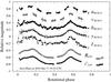 |
Fig. 1 Lightcurves of asteroid (21) Lutetia obtained at Calar Alto in March 17, using BUSCA instrument. The four Strömgren u,v,b,y and a Cousins-I filters are shown. Additionally, two lightcurves obtained at Lulin Observatory in March 19, using Cousins-R and Sloan i′ filters are also shown. |
In both cases, data reduction was performed using IRAF standard procedures (Tody 1993), including bias subtraction and flat field correction. Unfortunately, none of the observations were performed under good photometric conditions, so we were unable to do standard calibration, and no colour information is available. Nevertheless, we performed relative aperture photometry, using several reference stars in the same field on each night, and results were compared to ensure that no intrinsic short-term variability of the stars was introduced. We finally computed the average of the asteroid’s relative photometry obtained with all the selected stars. Lightcurves obtained with the BUSCA filters on March 17 and the two filters used for LOT observations (March 19) are shown in Fig. 1. Error bars correspond to 1σ deviation from the computed mean relative magnitude. The lightcurve obtained with filter I seems to be slightly different from the others. We can see a “depression” between rotational phase 0.52 and 0.56, and a significant decrease in brightness beyond 0.7. However, we do not see any of these features in the lightcurves obtained using filter i′, so we believe those apparent features should not be interpreted as true variations. Weather conditions were superior during the observations made on March 19, 20, and 21 at Lulin Observatory, so lightcurves with filters R and i′ have smaller dispersions.
2.2. Spectroscopy
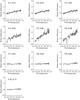 |
Fig. 2 Reflectance spectra of asteroid (21) Lutetia in the visible, normalised to unity at 0.55 μm. The spectra are labelled as in Table 1. The numbers correspond to the asteroid’s rotational phase at which they were taken. |
Visible spectra were obtained with the Calar Alto focal reducer and faint object spectrograph CAFOS on two nights. CAFOS is equipped with a 2048 × 2048 pixel blue-sensitive CCD and a plate scale of 0.53′′/pixel. We used the R-400 grism, giving a wavelength coverage from about 0.45 to 0.95 μm, and a dispersion of 9.7 Å/ per pixel (R ~ 400). A 1.5′′ slit was employed, oriented in the parallactic angle to correct for differential refraction effects, and the tracking was at the asteroid’s proper motion. Two acquisitions, between which the object was offset in the slit direction (positions A and B), were obtained. Pre-processing of the CCD images included bias and flat field correction. The extraction of 1D spectra from 2D images was carried out after the sky background subtraction (A − B), as described in Duffard & Roig (2009). Wavelength calibration was applied using Cd, Hg, and Rb lamps. To obtain the asteroid’s reflectance spectra, we observed three solar analogue stars from the Landolt catalogue (Landolt 1992) at similar airmass as the asteroid: SA 105-56, SA 107-684, and SA 110-361. Final reflectance spectra were normalised to unity at 0.55 μm. Observational details can be seen in Table 1, where the starting UT, Julian date (JD), airmass, and total on-object exposure time are indicated. Each spectrum listed in Table 1 corresponds to the sum of two (2x) individual spectra, obtained from one (A − B) subtraction, and can be seen in Fig. 2.
 |
Fig. 3 Same as Fig. 2, but for the near-infrared range. Spectra are normalised to unity at 1.6 μm. Last plot shows all the spectra offset vertically. |
Low resolution near-infrared spectra were taken with the 3.6 m Telescopio Nazionale Galileo (TNG) on two nights, using the low resolution mode of NICS (Near Infrared Camera Spectrograph), a multi-mode instrument based on a HgCdTe Hawaii 1024 × 1024 array. All spectroscopic modes use the large field (LF) camera, which has a plate scale of 0.25′′/pixel. We employed a 1.5′′ slit, and the Amici prism disperser, covering the 0.8–2.5 μm spectral range. As for the visible observations, the slit was oriented in the parallactic angle, and the tracking was at the asteroid’s proper motion. The acquisition consisted of two series of short exposure images, offsetting the object between positions A and B in the slit direction. This process was repeated and a number of ABBA cycles were acquired. The observational method and reduction procedure followed de León et al. (2010). Standard bias and flat field correction were applied to the images. From each ABBA cycle, we obtained two individual AB images, after subtracting consecutive A and B exposures. After the extraction of 1D spectra and wavelength calibration, we divided the asteroid’s spectrum by the spectra of the solar analogue stars SA 98-978, SA 102-1081, SA 107-998, and SA 110-361, observed at the same airmass as the object. The final reflectance spectra were normalised to unity at 1.6 μm, and are listed in Table 1, as well as their observational details. Each spectrum was obtained by averaging two (2 × ) or four (4 × ) AB individual spectra and can be seen in Fig. 3.
3. Results and discussion
We inspected the time-resolved observations in each filter to compute the rotational period of the asteroid, using the Lomb technique (Lomb 1976) as implemented by Press et al. (1979). The highest quality and longer observations, which were those acquired using the Cousins-R filter acquired at LOT (19, 20, 21 March), provided a rotational period of 8.16 ± 0.08 h. We also computed the rotational period using observations made with Sloan-i′ filter during the same nights, obtaining the same value. Our result is in good agreement with the previously published results, which gave a period of P = 8.16545 (Torppa et al. 2003). Figure 4 shows the combined lightcurves used to infer the rotational period, covering a complete rotation. Julian dates, rotational phases, and relative magnitudes for each night are presented in Table 2. It is clearly seen that the asteroid’s lightcurve has two asymmetric minima, with a mean peak-to-peak amplitude of 0.25 ± 0.05 mag. The J2000.0 ecliptic coordinates of the latest pole solution, computed from OSIRIS images (Jorda et al. 2010), are  and
and  . Following this pole solution, our observations were made with an aspect angle of ξ ~ 72°, i.e., Lutetia was in a near equatorial aspect. Nedelcu et al. (2007) observed Lutetia with a similar aspect angle and obtained an amplitude of 0.27 mag, in good agreement with our results.
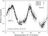 |
Fig. 4 Combined lightcurve of asteroid (21) Lutetia using photometric data in R broadband filter at different observing nights (March 19, 20, and 21, see Table 1). The zero rotational phase was chosen to occur at JD = 2 455 273.3094 (March 17 at 19:25 UTC). The rotational period inferred from this combined lightcurve was derived to be P = 8.16 ± 0.08 h. |
We can see in Fig. 1 that, considering the dispersion in the data of some of the lightcurves, they all have a similar behaviour, and no major differences are found among them. We note that in the combined lightcurve in Fig. 4, and in almost all the lightcurves obtained using different filters, we can observe a “depression”, a small-scale magnitude variation marked in the figure, between 0.08 and 0.15 rotational phases. This feature can be associated with both a variation in the albedo or a change in the topography (most likely a crater), although the second interpretation is preferred, as albedo spots are rarely detected among asteroids.
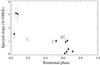 |
Fig. 5 Spectral slope S′ computed in the range 0.5–0.9 μm for the visible spectra (dots), and in the range 0.9–1.8 μm for the near-infrared (open squares) versus rotational phase. Visible and near-infrared spectra are normalised to unity at 0.55 and 1.6 μm respectively. |
With this result in mind, a month after the photometric observations we obtained visible and near-infrared spectra of the asteroid during the rotational phase (around 0.1) when this “depression” was detected. We also took spectra at another rotational phase (around 0.6), for comparison purposes. Each visible and near-infrared spectrum obtained is shown in Figs. 2 and 3, respectively, labelled by their corresponding identifier and rotational phase. For visible spectra, we observe a significant difference between those taken at 0.1 (V4, V5, V6) and the rest of spectra. To quantify this variation, we computed the spectral slope S′ between 0.5 and 0.9 μm for all the spectra. The obtained values are shown in Table 3 and plotted against rotational phase in Fig. 5. Visible spectra taken around 0.1 have redder slopes. However, they also have a higher dispersion, as they were observed at a higher airmass (see Table 1). Therefore, caution must be taken when interpreting this result, as the effect of differential refraction is higher, and its correction is more critical at visible wavelengths. Nevertheless, the difference in spectral slope at these two rotational phases can be tentatively interpreted in terms of surface inhomogeneities, as we are observing different portions of the surface of the asteroid. These inhomogeneities could be associated with differences in mineralogical composition or be the effect of materials processed to different degrees and then exposed in a crater area.
If we analyse each individual spectrum, we can see an absorption band centred at 0.58–0.60 μm in the V4, V5, and V6 spectra (this last one being significantly deeper). This absorption band has been reported by other authors (Lazzarin et al. 2004; Vernazza et al. 2009; Perna et al. 2010) and detected in the spectra of enstatite chondrites, as well as in minerals produced by aqueous alteration of silicates. Another potential absorption feature centred around 0.78–0.79 μm is seen in V1, V2, and V3 spectra, and is associated with the presence of ferrous and ferric iron in various oxides (crystal field transition Fe3+). These type of features related to oxidation are also observed in the spectra of C and M type asteroids (Busarev 2002). Finally, a broad and shallow absorption band centred around 0.65 μm is marginally present in the series V7-V10, and is also attributable to aqueous altered materials on the surface of the asteroid.
For near-infrared spectra (see Fig. 5), we are unable to discern any significant differences between the data obtained at different rotational phases. As for the visible spectra, we computed the spectral slope S′ between 0.9 and 1.8 μm. The values obtained are listed in Table 3 and plotted against rotational phase in Fig. 5 (open squares). We do not see any significant difference in the spectral slopes. Individual spectra are also very similar to each other. Nevertheless, a very weak absorption feature centred around 0.80–0.85 μm, which is barely detectable, can be distinguished in the IR1 and IR2 spectra (see the arrows in Fig. 3). This absorption feature was previously reported by Lazzarin et al. (2004) and Belskaya et al. (2010), and is attributed to charge transfer transitions in oxidised iron.
Computed spectral slopes in the range 0.5–0.9 μm for visible spectra and 0.9–1.8 for near-infrared spectra.
4. Conclusions
We have compiled photometric lightcurves using several filters and spectra in the visible and near-infrared range for the asteroid (21) Lutetia, just three months before the Rosetta fly-by. Taking into account the results of our data analysis presented here, we have been able to draw some conclusions that support the findings derived from previous observations:
-
1.
From the photometric lightcurves acquired during threeconsecutive nights, we have obtained a rotational period of8.16 ± 0.08 h, in good agreement with previous determinations. The rotational lightcurve of the asteroid has two asymmetric minima, with a peak-to-peak amplitude of 0.25 ± 0.05 mag.
- 2.
The lightcurves obtained using different filters have similar properties. We can see a small-scale magnitude variation in all of them, some sort of “depression” around 0.1 rotational phase. This feature could be associated with both variations in mineralogical composition or a shadowing effect caused by the topography of the surface.
- 3.
Visible spectra were taken around 0.1 and 0.6 rotational phases, and spectral slope was computed in the range 0.5–0.9 μm. Spectra taken at a 0.1 rotational phase had redder slopes, which are indicative of differences in mineralogical composition or the level of processing of materials in a crater area. For the near-infrared spectra, we have been unable to discern any significant variation in the spectral slope with rotational phase. Some absorption features were detected in both visible and near-infrared spectra, and were attributed to the action of aqueous alteration on minerals, namely enstatite, phyllosilicates, or oxidised iron. However, infrared data obtained during the fly-by almost exclude the presence of hydrated minerals on the surface of the asteroid.
Note added in proof Fly-by of asteroid (21) Lutetia was successfully completed on July 10, 2010. Images taken by OSIRIS instrument on-board the spacecraft show that the asteroid is covered with many craters, varying in size. They also show a large crater located close to the asteroid’s equator, expanding from -10° to 40° in latitude (Marchi, priv. comm.). That crater could account for the small scale variation in magnitude observed in the ligthcurves presented in this paper.
Acknowledgments
This research has been partially funded by the Ministerio de Ciencia e Innovación through the project AYA 2009-08011. J. de León and Z.-Y. Li. acknowledge a post-doctoral contract by the Junta de Andalucía research project PE07-TIC2744. R. Duffard acknowledges financial support from MICINN (contract Ramón y Cajal). We thank the Centro Astronómico Hispano-Alemán (CAHA) for the facilities and support made available at Calar Alto. We also thank all staff and observers of the Lulin telescope for various arrangements in realizaing this observation. This paper is based on observations made with the Italian Telescopio Nazionale Galileo (TNG) operated on the island of La Palma by the Centro Galileo Galilei of the INAF (Instituto Nazionale di Astrofisica).
References
- Barucci, M. A., Fulchignoni, M., Fornasier, S., et al. 2005, A&A, 430, 313 [NASA ADS] [CrossRef] [EDP Sciences] [Google Scholar]
- Belskaya, I. N., Fornasier, S., Krugly, Yu. N., et al. 2010, A&A, 515, A29 [NASA ADS] [CrossRef] [EDP Sciences] [Google Scholar]
- Birlan, M., Vernazza, P., Fulchignoni, M., et al. 2006, A&A, 454, 677 [NASA ADS] [CrossRef] [EDP Sciences] [Google Scholar]
- Busarev, V. V. 2002, Sol. Syst. Res., 36, 35 [NASA ADS] [CrossRef] [Google Scholar]
- Carvano, J. M., Barucci, A., Delbó, M., et al. 2008, A&A, 479, 241 [NASA ADS] [CrossRef] [EDP Sciences] [Google Scholar]
- de León, J., Licandro, J., Serra-Ricart, M., et al. 2010, A&A, 517, A23 [NASA ADS] [CrossRef] [EDP Sciences] [Google Scholar]
- Duffard, R., & Roig, F. 2009, Planet. Space Sci., 57, 229 [NASA ADS] [CrossRef] [Google Scholar]
- Fornasier, S., Barbieri, C., Barucci, M. A., et al. 2010, BAAS, 42, 1032 [NASA ADS] [Google Scholar]
- Jorda, L., Lamy, P., Besse, S., et al. 2010, BAAS, 42, 1043 [NASA ADS] [Google Scholar]
- Lamy, P. L., Groussin, O., Fornasier, S., et al. 2010, A&A, 516, A74 [NASA ADS] [CrossRef] [EDP Sciences] [Google Scholar]
- Landolt, A. U. 1992, AJ, 104, 340 [NASA ADS] [CrossRef] [Google Scholar]
- Lazzarin, M., Marchi, S., Magrin, S., et al. 2004, A&A, 425, L25 [Google Scholar]
- Lazzarin, M., Marchi, S., Moroz, L. V., & Magrin, S. 2009, A&A, 498, 307 [NASA ADS] [CrossRef] [EDP Sciences] [Google Scholar]
- Lomb, N. R. 1976, Ap&SS, 39, L447 [NASA ADS] [CrossRef] [Google Scholar]
- Lupishko, D. F., & Mohamed, R. A. 1996, Icarus, 119, 209 [NASA ADS] [CrossRef] [Google Scholar]
- Mueller, M., Harris, A. W., Bus, S. J., et al. 2006, A&A, 447, 1153 [NASA ADS] [CrossRef] [EDP Sciences] [Google Scholar]
- Nedelcu, D. A., Birlan, M., Vernazza, P., et al. 2007, A&A, 470, 1157 [NASA ADS] [CrossRef] [EDP Sciences] [Google Scholar]
- Perna, D., Dotto, E., Lazzarin, M., et al. 2010, A&A, 513, L4 [NASA ADS] [CrossRef] [EDP Sciences] [Google Scholar]
- Press, W. H., Teukolsky, S. A., Vetterling, W. T., & Flannery, B. P. 1992, in Numerical Recipes in Fortran: the art of scientific computing, 2nd edn. (London: Cambridge University Press), 569 [Google Scholar]
- Tody, D. 1993, in Astronomical Data Analysis Software and Systems II, ed. R. J. Hanisch, R. J. V., Brissenden, & J. Barnes (San Francisco: Astron. Soc. of the Pacific), 173 [Google Scholar]
- Torppa, J., Kaasalainen, M., Michalowski, T., et al. 2003, Icarus, 164, 346 [NASA ADS] [CrossRef] [Google Scholar]
- Vernazza, P., Brunetto, R., Binzel, R. P., et al. 2009, Icarus, 202, 477 [NASA ADS] [CrossRef] [Google Scholar]
All Tables
Computed spectral slopes in the range 0.5–0.9 μm for visible spectra and 0.9–1.8 for near-infrared spectra.
All Figures
|
Fig. 1 Lightcurves of asteroid (21) Lutetia obtained at Calar Alto in March 17, using BUSCA instrument. The four Strömgren u,v,b,y and a Cousins-I filters are shown. Additionally, two lightcurves obtained at Lulin Observatory in March 19, using Cousins-R and Sloan i′ filters are also shown. |
| In the text | |
|
Fig. 2 Reflectance spectra of asteroid (21) Lutetia in the visible, normalised to unity at 0.55 μm. The spectra are labelled as in Table 1. The numbers correspond to the asteroid’s rotational phase at which they were taken. |
| In the text | |
|
Fig. 3 Same as Fig. 2, but for the near-infrared range. Spectra are normalised to unity at 1.6 μm. Last plot shows all the spectra offset vertically. |
| In the text | |
|
Fig. 4 Combined lightcurve of asteroid (21) Lutetia using photometric data in R broadband filter at different observing nights (March 19, 20, and 21, see Table 1). The zero rotational phase was chosen to occur at JD = 2 455 273.3094 (March 17 at 19:25 UTC). The rotational period inferred from this combined lightcurve was derived to be P = 8.16 ± 0.08 h. |
| In the text | |
|
Fig. 5 Spectral slope S′ computed in the range 0.5–0.9 μm for the visible spectra (dots), and in the range 0.9–1.8 μm for the near-infrared (open squares) versus rotational phase. Visible and near-infrared spectra are normalised to unity at 0.55 and 1.6 μm respectively. |
| In the text | |
Current usage metrics show cumulative count of Article Views (full-text article views including HTML views, PDF and ePub downloads, according to the available data) and Abstracts Views on Vision4Press platform.
Data correspond to usage on the plateform after 2015. The current usage metrics is available 48-96 hours after online publication and is updated daily on week days.
Initial download of the metrics may take a while.