| Issue |
A&A
Volume 527, March 2011
|
|
|---|---|---|
| Article Number | A46 | |
| Number of page(s) | 6 | |
| Section | The Sun | |
| DOI | https://doi.org/10.1051/0004-6361/201014384 | |
| Published online | 24 January 2011 | |
Downstream structure and evolution of a simulated CME-driven sheath in the solar corona
1
Institute for the Study of Earth, Oceans, and Space, University of New
Hampshire,
Durham,
NH
03824,
USA
e-mail: yong.liu@unh.edu
2
Department of Physics and Astronomy, George Mason
University, Fairfax,
VA
22030,
USA
e-mail: mopher@gmu.edu
3
School of Earth and Space Science, University of Science and
Technology of China, Hefei, Anhui
230026, PR
China
e-mail: ymwang@ustc.edu.cn
4
Department of Atmospheric, Oceanic, and Space Sciences, University
of Michigan, 2455 Hayward
Street, Ann Arbor,
MI
48109-2143,
USA
e-mail: tamas@umich.edu
Received:
8
March
2010
Accepted:
30
June
2010
Context. The transition of the magnetic field from the ambient magnetic field to the ejecta in the sheath downstream of a coronal mass ejection (CME) driven shock is analyzed in detail. The field rotation in the sheath occurs in a two-layer structure. In the first layer, layer 1, the magnetic field rotates in the coplanarity plane (plane of shock normal and the upstream magnetic field), and in layer 2 rotates off this plane. We investigate the evolution of the two layers as the sheath evolves away from the Sun.
Aims. In situ observations have shown that the magnetic field in the sheath region in front of an interplanetary coronal mass ejection (ICME) form a planar magnetic structure, and the magnetic field lines drape around the flux tube. Our objective is to investigate the magnetic configuration of the CME near the sun.
Methods. We used the space weather modeling framework (SWMF), a 3D magnetohydrodynamics (MHD) simulation code, to simulate the propagation of CMEs and the shock driven by it.
Results. We find that close to the Sun, layer 2 dominates the width of the sheath, diminishing its importance as the sheath evolves away from the Sun, in agreement with observations at 1 AU.
Key words: magnetohydrodynamics (MHD) / magnetic fields / Sun: coronal mass ejections (CMEs)
© ESO, 2011
1. Introduction
A coronal mass ejection (CME) is now understood to be an eruption of magnetized plasma from the Sun of energy up to 1032 erg. Sometimes a CME has a speed higher than the fast-mode magnetosonic speed in the background solar wind, and a shock is driven in front of it (Hudson et al. 2006). The CME is of great importance to space weather for at least two reasons: 1) some CMEs come across Earth and have great impact on Earth′s magnetosphere (see review, Webb and Gopalswamy 2006); 2) a fraction of CME-driven shocks of large Mach number are able to generate very high-energy (GeV) particles, which are hazardous to life and instruments onboard spacecrafts in outer space (Roussev et al. 2004; Lee 2005). Remote sensing of CMEs near the Sun demonstrate that 30% of CMEs have a bright front and a dark cavity (Hundhausen 1987). The bright front is now known as a higher-density plasma and the dark cavity corresponds to the ejected flux rope. In this work we focus only on the CMEs that have a three-part structure and drive a shock ahead.
In situ observations of ICME, the counterpart of CME at 1 AU, reveal detailed information about the transition from the sheath to the ejecta. At the lower boundary of the sheath, the magnetic field lines drape around the flux rope (Kaymaz & Siscoe 2006). In-depth analysis of ICME in relationship to magnetic field draping were also performed by Liu et al. (2006), and a comparison with MHD simulations was conducted by Liu et al. (2008a). Observations of ICMEs have found planar magnetic structures (PMS), which are characterized by an ordering of magnetic fields into laminar sheets in the sheath (Nakagawa et al. 1989). Other research suggests that PMSs form by the processes of the magnetic field draping around the magnetic cloud (Farrugia et al. 1990; Neugebauer et al. 1993; Jones et al. 2003). Studies by Kataoka et al. (2005) demonstrated that the generation of PMS is related to both the plasma −β (the ratio of the magnetic pressure to the thermal pressure) and the shock magnetic angle θBn (the angle between the shock normal and the magnetic field) downstream of the shock. These studies establish the magnetic structure configuration in the sheath region for ICMEs. However, for CMEs near the sun, the magnetic configuration in the sheath and its evolution are not well understood.
Manchester et al. (2005) simulated the CME with an earlier version of the Space Weather Modeling Framework (SWMF) developed at the University of Michigan (Toth et al. 2005). In their simulation, the heating of the solar wind is assumed to be a given function of latitude. Their simulation studied a CME from a few solar radii to 1 AU, focusing on the evolution of a large-scale configuration of the magnetic field connection from the corona to the far interplanetary space. In this paper, we investigate the transition from the sheath to the flux rope for a simulated CME in the lower solar corona with an improved SWMF, in which a realistic solar wind is generated with a variable polytropic index. In particular, we investigate the rotation of the magnetic field in the sheath region and reveal that the rotation of the magnetic field has a two-layer structure in the sheath. The paper is arranged as follows: in Sect. 2, we present our simulation; in Sect. 3, we discuss sheath features, such as the density change and show that these features match the features of ICMEs. Section 4 discusses the rotation of the magnetic field in the sheath. Section 5 presents conclusions and discussions.
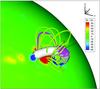 |
Fig. 1 The inserted flux rope and the active region on the sun. The color on the spherical surface represents the magnetic field on the surface of the sun. The flux rope is represented by the isosurface of the current I = 200 mA. The pink lines are the magnetic field lines around the flux rope. The black line illustrates the line around which the grids are refined and the density, temperature, and magnetic field are also sampled for detailed investigation. |
2. Simulation
The space weather modeling framework, SWMF, integrates physical models for different domains in the Sun-Earth system (Toth et al. 2005). The component SC models the solar corona extending from the Sun to 24 Rs (Rs being the solar radii) from the sun, the component IH models the inner heliosphere extending until 250 Rs. Each component is coupled with the other component by means of a coupling interface. The SWMF can perform/implement adaptive mesh refinement (AMR), which allows the user to refine the region dominated by physical processes of small spatial scales, e.g., regions around a shock or the current sheet.
Our simulation uses only the component SC that models the solar corona. First we simulate a steady solar wind using a semi-empirical model (Roussev et al. 2003; Cohen et al. 2007). The problem of solar wind heating is a major challenge (see Hollweg 1990). Global models employ different approaches to implement a more realistic solar wind. Cohen et al. (2008) employ an empirical approach, parameterizing the heating by a variable polytropic index. The solar wind speed at 1 AU is determined using the Wang-Sheeley-Arge model, in which the MDI synoptic chart of the Carrington rotation 1922 is adopted to extrapolate the coronal magnetic field (Arge & Pizzo 2000; Arge et al. 2003, 2004). This Carrington rotation was chosen because it is at a solar minimum and the magnetic structure for the ambient solar wind is simpler. The speeds on the Sun′s surface are determined using the Bernouli equation. Combined with the temperature on the Sun, the speed at the Sun’s surface is used to determine the distribution of polytropic indices through the pressure function. These derived polytropic indices are then incorporated into self-consistent MHD equations. The distribution of the polytropic indices obtained is discussed in Cohen et al. (2008). After the MHD equations and the boundary conditions on the sun are set up, the code iterates 13 000 steps to reach a steady state. The solar wind speed and the magnetic field on the ecliptic plane are shown in Fig. 1 of Liu et al. (2008b).
The steady state generated is set up as a background configuration for the solar corona. A modified Titov-Demoulin flux rope (Titov & Demoulin 1999) is placed near an active region around the solar equator. We refined the grid around the center of the shock to have a size of 0.03 Rs. Figure 1 (adapted from Liu et al. 2008b) shows the flux rope, the line around the area where the mesh is refined and the magnetic field on the surface of the Sun. Shortly after the initial setup, the CME propagates at a speed of 400 km s-1 and accelerate to 600 km s-1 in about 50 min. The ambient Alfvén speed at the region where CME propagates is less than 300 km s-1. The steady-state solar wind, the initiation of the CME, the propagation and acceleration of the CME, the evolution of the CME-driven shock, and the post-shock compression were presented in Liu et al. (2008b).
 |
Fig. 2 The plot of density, temperature, and angle of the magnetic field versus (vs.) position for times a) t = 20 min, b) t = 30 min, and c) t = 40 min. The dashed lines mark the region of the sheath characterized by the compressed plasma. |
3. Sheath
The transition from the interplanetary field to the ejecta has been investigated extensively using in situ observations on ICMEs, the interplanetary manifestations of CMEs (Kaymaz & Siscoe 2006; Liu et al. 2006, 2008a). The observed properties used to identify sheaths include density change and magnetic field rotation. (Klein & Burlaga 1982; Liu et al. 2006; Richardson & Cane 1995). These features are measured at 1 AU. In this paper, we analyze the sheath characteristics near the Sun and study its evolution as the sheath propagates from the Sun. This study is very important because through the study of the internal structure of a CME we gain insight on the acceleration of particles. It is known that energetic particles are accelerated predominantly in the lower corona (Lee 2005).
To quantify these features, we sample the data on a radial line going through the middle of the flux rope (X = 1.08 Rs, Y = 0.27 Rs, Z = 0.11 Rs). The coordinates X, Y, and Z are in the heliographic rotational system (HGR), the same as the coordinate system used in the calculation. In Fig. 2, the density, the temperature, and the angles θB and φB, which are the zenith and azimuthal angle of the magnetic field, respectively, are plotted versus (vs.) R (the distance to the center of the sun) for t = 20, 30, and 40 min. The temperatures were obtained from the pressure and mass density in the simulated sheath. The two straight dashed lines mark the sheath region of compressed plasma ahead of the flux rope (ejecta), which is characterized by low-density plasma.
The density decreases to about one fourth of the maximum density toward the ejecta. In addition to the decrease in density, the zenith angle of the magnetic field θB increases over 60 degrees at the lower boundary of the sheath, which implies that the magnetic field rotates over large angles. This rotation is in additional to the usual rotation seen as the spacecraft travels through the flux rope (ejecta). These two features are consistent with the ICME observations at 1 AU (Kaymaz & Siscoe 2006). The temperature in the sheath is lower than the temperature in the flux rope, which is opposite to the observed temperatures. The Titov-Demoulin flux rope is very diffusive, and as the flux rope propagates away from the Sun, diffusion tends to dissipate the magnetic flux converting it into heat. This numerical artefact can be avoided only by employing extremely high resolution all along the flux rope, which is numerically forbidden. We refined the grid in the Sun-Earth line with 0.03 Rs. Since we focus mainly on the magnetic evolution from the sheath to the flux rope, we assume qualitatively that our analysis and results hold.
 |
Fig. 3 The magnetic field lines drape around flux rope. The green surface is an isosurface of density 10-17 g/cm-3, which represents the flux rope. The red lines are the magnetic field lines. The colored sphere on the left represents part of the Sun′s surface. The blue and red area is the active region where we inserted a flux rope to initiate a CME. The pink line indicates the line from which we sampled the data. |
Another property of the observed ICMEs is that the magnetic field lines drape around the ICME (Gosling & McComas 1987; McComas et al. 1989). Figure 3 shows the flux rope, several magnetic field lines, and part of the Sun′s surface at a time t = 20 min after the CME initiation. The distance from the shock to the center of the sun (Ds) is 2.5 Rs. The light green surface in Fig. 3 is an isosurface of density 10-17 g/cm-3. Inside the surface, the density is lower than the surrounding ambient corona. Thus, the surface represents the flux rope and the lower boundary of the sheath. The red lines are the magnetic field lines; the pink line goes through the center of the flux rope and is the line from which we sample the data. The colored spherical surface is the surface of the sun; the contours on the surface represent the photosphere magnetic field; the blue and red area is the active region where we insert the flux rope to initiate a CME. The magnetic field lines drape around the flux rope just as those observed magnetic field lines do in front of an ejecta.
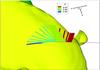 |
Fig. 4 Magnetic-field-line rotation in front of the flux rope. The yellow surface represents the flux rope and the colored lines represent the magnetic field lines ahead of it. The color on the lines represents R, the distance from the center of the sun normalized by Rs. |
4. Magnetic field rotation
To investigate how the magnetic fields change their configuration as they evolve from the ambient magnetic field to align themselves with the magnetic field in the flux rope, the magnetic field lines in the sheath at t = 30 min (Ds = 3Rs) are plotted in Fig. 4. The yellow surface (density isosurface of 5 × 10-18 g/cm-3) represents the flux rope, as we mentioned in previous section. The dark brown magnetic field lines are ahead of the shock and the light green lines are behind the shock. These two groups of magnetic field lines are in the coplanarity plane (the plane defined by the shock normal and the magnetic field at the shock). The lighter blue lines, which are in the sheath and closer to the flux rope, rotate off the coplanarity plane as they approach the flux rope. However, although these field lines rotate, they remain in a plane parallel to the shock plane.
To quantify the field lines rotation from the coplanarity plane, we define a new coordinate
system (x′y′z′). The z′
axis is along the shock normal; the x′ axis is along the projection of the
upstream magnetic field on the shock plane. Therefore, the x′
-z′ plane is the coplanarity plan and the y′ axis is
chosen to complete the coordinate. The configuration of the coordinates
(x′y′z′), the zenith angle
 , and the
azimuth angle are shown in
Fig. 5. The zenith angle
measures the
rotation inside the coplanarity plane, and the azimuth angle
, and the
azimuth angle are shown in
Fig. 5. The zenith angle
measures the
rotation inside the coplanarity plane, and the azimuth angle
 measures the
rotation off it. In the sheath region, the angles and
are plotted for
the CME at t = 20, 30, and 40 min in Fig. 6 (Ds is 2.5 Rs,
3 Rs, and 3.5 Rs, respectively).
We define two layers: layer 1 is close to the shock and layer 2 is close to the flux rope,
as shown in Fig. 6. In layer 1, the azimuth angle
stays at zero
and the zenith angle changes. In
layer 2, the azimuth angle
measures the
rotation off it. In the sheath region, the angles and
are plotted for
the CME at t = 20, 30, and 40 min in Fig. 6 (Ds is 2.5 Rs,
3 Rs, and 3.5 Rs, respectively).
We define two layers: layer 1 is close to the shock and layer 2 is close to the flux rope,
as shown in Fig. 6. In layer 1, the azimuth angle
stays at zero
and the zenith angle changes. In
layer 2, the azimuth angle  increases from
zero to an angle larger than 80°; however, the zenith angle
increases from
zero to an angle larger than 80°; however, the zenith angle
 varies in a
small range around 90° within the shock plane. The flux rope begins at the lower boundary of
layer 2.
varies in a
small range around 90° within the shock plane. The flux rope begins at the lower boundary of
layer 2.
 |
Fig. 5 The configuration of the x′y′z′ coordinate system, zenith angle θ′, and azimuth angle φ′. The z′ axis is chosen along shock normal, the x′ is the projection of the upstream magnetic field on the shock plane, and y′ completes the left hand (or right hand) coordinate system. |
 |
Fig. 6 The plot of density and the rotation angles θ′, φ′, for a) t = 20, b) t = 30, and c) t = 40 min. The dashed lines mark the layer close to the flux rope in which all the transitions happen. The magnetic field lines rotate to drape around the flux rope in this region. |
Figure 7 shows the evolution of the width of the two layers normalized by the width of the sheath as a function of Ds. In the distance range Ds = 2.5−2.7 Rs, the layer 2 occupies 90% of the sheath; for Ds ≥ 3 Rs, layer 2 occupies less than 50% of the sheath. As the CME propagate away from the Sun there is a tendency for layer 2 to diminish and layer 1 to grow. Closer to the Sun, the magnetic field forces dominate. As the shock propagates outward, the current diffuses and layer 1 grows as layer 2 diminishes.
5. Discussions and conclusions
We have presented a CME simulation performed with a 3D MHD AMR code (SWMF) and investigated the magnetic structure of the sheath between the flux rope and the CME-driven shock. Our simulation, focused on the transition of the magnetic field lines, is consistent with most observed ICMEs in terms of density increase, magnetic field rotation, and magnetic field draping around the magnetic cloud (Kaymaz & Siscoe 2006; Liu et al. 2006). We have investigated the transition of the magnetic field from the shocked solar wind to its alignment with the flux rope and the evolution of the CME sheath. We draw the following conclusions:
-
1.
For the CME near the Sun, the magnetic field lines drape aroundthe flux rope. Similarly observed ICMEs have magnetic fieldlines that drape around them at 1 AU (Kaymaz &Siscoe 2006; Liu et al. 2006).
-
2.
The sheath between the shock and the flux rope can be divided into two layers: layer 1 and layer 2. The two layers describe the transition of the ambient magnetic field to the fields draping around the flux rope (ejecta). The evolution of the magnetic field lines in the two layers is different. In layer 1, the magnetic field lines remain in the coplanarity layer as if they are unaffected by the draping field line. In layer 2, the field lines rotate away from the coplanarity plane and align themselves with the magnetic field in the flux rope. Jones et al. (2002) proposed a scenario for the evolution of field lines in ICMEs. Here we explore this in 3D near the Sun and demonstrate that the field rotation occurs in two stages, and at each stage the rotation happens in one plane. This result is also consistent with the schematic plot in Fig. 1 of Liu et al. (2006).
-
3.
The relative width of the two layers with respect to the width of the sheath has also been calculated. Layer 2 dominates the sheath at Ds ≤ 3 Rs, and after that, layer 2 occupied less than 50% of the sheath. In layer 1, the change in magnetic field lines is dominated by magnetic field forces in the shock plane. The flow that is very close to the shock remains mainly aligned in radial direction but slightly deflected toward the meridional direction, starting to deflect around the flux rope further away from the shock (Liu et al. 2008a). The deflected flows drag the field lines off the coplanarity plane and form layer 2, while the field lines remain in the coplanarity plane in layer 1. Additional investigations are required to determine the structure evolution of the sheath, such as what controls the normalized width of the layers and why the widths change with time. The diminished importance of layer 2 with time could be related to the change in magnetic forces that cease to dominate as a given CME evolve away from the Sun (Liu et al. 2008b).
The two-layer structure of the sheath behind the CME-driven shock in the solar corona was not detected in the ICME observations at 1 AU. A possible corresponding part of the layer 2 at 1 AU is the depletion layer, which is far narrower than the width of the sheath (Liu et al. 2006). This idea is consistent with our observation of the diminishing importance of layer 2 as the CME evolves away from the Sun at 1 AU. There are several possible explanations of layer 2′s being small at 1 AU: the two layer structure has a latitude dependence that is stronger at the nose, and observations of ICMEs are made mostly in the flank. We expect a latitude dependence of layers 1 and 2 since, as we go away from the axis of symmetry of the shock, the flows have a stronger azimuthal component and drag the frozen-in magnetic field away from the coplanarity plane. We also note that layer 1 behaves like PMS since the magnetic fields remain in the coplanarity plane. However, we have been unable to predict in which situations the PMSs can be observed at 1 AU or further. Other factors neglected in our simulations, such as turbulence, may also explain why the two-layer structure is not observed at 1 AU.
 |
Fig. 7 The plot of width normalized by the sheath width for each layer as a function of Ds, which is the location of the shock indicated by the distance from the center of the sun. The solid (dashed) line represents the width of layer 1(2). |
Acknowledgments
This work is supported by LWS NNG06GB53G, National Science Foundation CAREER Grant ATM-0747654 at George Mason University and NASA STEREO NAS5-00132 at University of New Hampshire. The authors would like to thank the staff at NASA Ames Research Center for the use of the Columbia supercomputers. Y. Liu also appreciates C. Goodwin’s help to correct the English in this article.
References
- Arge, C. N., & Pizzo, V. J. 2000, J. Geophys. Res., 105, 10, 465 [Google Scholar]
- Arge, C. N., Odstrcil, D., Pizzo, V. J., & Mayer, L. R. 2003, in Solar Wind Ten, AIP Conf. Proc., 679, 190 [Google Scholar]
- Arge, C. N., Luhmann, J. G., Odstrcil, D., Schrijver, C. J., & Li, Y. 2004, J. Atmos. Terr. Phys., 66, 1295 [Google Scholar]
- Cohen, O., Sokolov, I. V., Roussev, I. I., et al. 2007, ApJ, 654, L163 [NASA ADS] [CrossRef] [Google Scholar]
- Cohen, O., Sokolov, I. V., Roussev, I. I., & Gombosi, T. I. 2008, J. Geophys. Res. 113, A03104 [Google Scholar]
- Farrugia, C. J., Dunlop, M. W., Geurts, F., et al. 1990, Geophys. Res. Lett., 17, 1025 [NASA ADS] [CrossRef] [Google Scholar]
- Gosling, J. T., & McComas, D. J. 1987, Geophys. Res. Lett. 14, 355 [NASA ADS] [CrossRef] [Google Scholar]
- Hollweg, J. V. 1990, Comp. Phys. Rep., 12, 205 [Google Scholar]
- Hundhausen, A. J. 1987, Sixth International Solar Wind Conference, 181 [Google Scholar]
- Hudson, H. S., Bougeret, J.-L., & Burkepile, J. 2006, Space Sci. Rev., 123, 13 [NASA ADS] [CrossRef] [Google Scholar]
- Jones, G. H., Rees, A., Balogh, A., & Forsyth, R. J. 2002, Geophys. Res. Lett., 29, 1520 [NASA ADS] [CrossRef] [Google Scholar]
- Kataoka, R., Watari, S., Shimada, N., Shimazu, H., & Marubashi, K. 2005 Geophys. Res. Lett., 32, L12103 [CrossRef] [Google Scholar]
- Kaymaz, Z., & Siscoe, G. 2006, Sol. Phys., 239, 437 [NASA ADS] [CrossRef] [Google Scholar]
- Klein, L. W., & Burlaga, L. F. 1982, J. Geophys. Res., 87, 613 [Google Scholar]
- Manchester, W. B., Gombosi, T. I., De Zeeuw, D., et al. 2005, ApJ, 622, 1225 [NASA ADS] [CrossRef] [Google Scholar]
- Lee, M. A. 2005 ApJS, 158, 38 [NASA ADS] [CrossRef] [Google Scholar]
- Liu, Y., Richardson, J. D., Belcher, J. W., Kasper, J. C., & Skoug, R. M. 2006, J. Geophys. Res., 111, A09108 [NASA ADS] [CrossRef] [Google Scholar]
- Liu, Y., Manchester, W. B., Richardson, J. D., et al. 2008a, J. Geophys. Res., 113, A00B03 [CrossRef] [Google Scholar]
- Liu, Y. C.-M., Opher, M., Cohen, O., Liewer, P. C., & Gombosi, T. I. 2008b, ApJ, 680, 757 [NASA ADS] [CrossRef] [Google Scholar]
- McComas, D. J., Gosling, J. T., Bame, S. J., Smith, E. J., & Cane, H. V. 1989, J. Geophys. Res., 94, 1465 [NASA ADS] [CrossRef] [Google Scholar]
- Nakagawa, T., Nishida, A., & Saito, T. 1989, J. Geophys. Res., 94, 11761 [NASA ADS] [CrossRef] [Google Scholar]
- Neugebauer, M. 1993, J. Geophys. Res., 98, 9383 [NASA ADS] [CrossRef] [Google Scholar]
- Richardson I. G., & Cane, H. V. 1995, J. Geophys. Res., 100, 23397 [NASA ADS] [CrossRef] [Google Scholar]
- Roussev, I. I., Gombosi, T. I., Sokolov, I. V., et al. 2003, ApJ, 595, L57 [Google Scholar]
- Titov, V. S., & Demoulin, P. 1999, A&A, 351, 707 [NASA ADS] [Google Scholar]
- Toth, G., Sokolov, I. V., Gombosi, T. I., & Chesney, D. R., et al. 2005, J. Geophys. Res., 110, 12226 [NASA ADS] [CrossRef] [Google Scholar]
- Webb D. F., & Gopalswamy N. 2006, Solar Influence on the Heliosphere and Earth’s Environment: Recent Progress and Prospects, ed. N. Gopalswamy, & A. Battacharyya, 71 [Google Scholar]
All Figures
|
Fig. 1 The inserted flux rope and the active region on the sun. The color on the spherical surface represents the magnetic field on the surface of the sun. The flux rope is represented by the isosurface of the current I = 200 mA. The pink lines are the magnetic field lines around the flux rope. The black line illustrates the line around which the grids are refined and the density, temperature, and magnetic field are also sampled for detailed investigation. |
| In the text | |
|
Fig. 2 The plot of density, temperature, and angle of the magnetic field versus (vs.) position for times a) t = 20 min, b) t = 30 min, and c) t = 40 min. The dashed lines mark the region of the sheath characterized by the compressed plasma. |
| In the text | |
|
Fig. 3 The magnetic field lines drape around flux rope. The green surface is an isosurface of density 10-17 g/cm-3, which represents the flux rope. The red lines are the magnetic field lines. The colored sphere on the left represents part of the Sun′s surface. The blue and red area is the active region where we inserted a flux rope to initiate a CME. The pink line indicates the line from which we sampled the data. |
| In the text | |
|
Fig. 4 Magnetic-field-line rotation in front of the flux rope. The yellow surface represents the flux rope and the colored lines represent the magnetic field lines ahead of it. The color on the lines represents R, the distance from the center of the sun normalized by Rs. |
| In the text | |
|
Fig. 5 The configuration of the x′y′z′ coordinate system, zenith angle θ′, and azimuth angle φ′. The z′ axis is chosen along shock normal, the x′ is the projection of the upstream magnetic field on the shock plane, and y′ completes the left hand (or right hand) coordinate system. |
| In the text | |
|
Fig. 6 The plot of density and the rotation angles θ′, φ′, for a) t = 20, b) t = 30, and c) t = 40 min. The dashed lines mark the layer close to the flux rope in which all the transitions happen. The magnetic field lines rotate to drape around the flux rope in this region. |
| In the text | |
|
Fig. 7 The plot of width normalized by the sheath width for each layer as a function of Ds, which is the location of the shock indicated by the distance from the center of the sun. The solid (dashed) line represents the width of layer 1(2). |
| In the text | |
Current usage metrics show cumulative count of Article Views (full-text article views including HTML views, PDF and ePub downloads, according to the available data) and Abstracts Views on Vision4Press platform.
Data correspond to usage on the plateform after 2015. The current usage metrics is available 48-96 hours after online publication and is updated daily on week days.
Initial download of the metrics may take a while.