| Issue |
A&A
Volume 527, March 2011
|
|
|---|---|---|
| Article Number | A86 | |
| Number of page(s) | 11 | |
| Section | Interstellar and circumstellar matter | |
| DOI | https://doi.org/10.1051/0004-6361/200913342 | |
| Published online | 31 January 2011 | |
3D numerical simulations of photodissociated and photoionized disks
1
Laboratório de Astrofísica Teórica e Observacional, DCET, Universidade
Estadual de Santa Cruz,
Rod. Ilhéus-Itabuna, km 16,
Ilhéus,
Bahia,
Brasil
e-mail: This email address is being protected from spambots. You need JavaScript enabled to view it.
, This email address is being protected from spambots. You need JavaScript enabled to view it.
2 Instituto de Ciencias Nucleares, UNAM, Ap. Postal 70-543, CU,
DF 04510, México
e-mail: This email address is being protected from spambots. You need JavaScript enabled to view it.
Received: 23 September 2009
Accepted: 20 December 2010
Abstract
Aims. In this work we study the influence of the UV radiation field of a massive star on the evolution of a disklike mass of gas and dust around a nearby star. This system has similarities with the proplyds seen in Orion.
Methods. We study disks with different inclinations and distances from the source, performing fully 3D numerical simulations. We use the YGUAZÚ-A adaptative grid code modified to account for EUV/FUV fluxes and non-spherical mass distributions. We treat H and C photoionization in order to reproduce the ionization fronts and photodissociation regions observed in proplyds. We also incorporate a wind from the ionizing source, in order to investigate the formation of the bow shock observed in several proplyds. We examine density and Hα maps, as well as the mass loss rates in the photoevaporated winds.
Results. Our results show that a photoevaporated wind propagates from the disk surface and becomes ionized after an ionization front (IF) seen as a bright peak in the Hα maps. We follow the development of an HI region inside the photoevaporated wind which corresponds to a photodissociated region (PDR) for most of our models, except those without a FUV flux. For disks that are at a distance from the source d ≥ 0.1 pc, the PDR is thick and the IF is detached from the disk surface. In contrast, for disks that are closer to the source, the PDR is thin and not resolved in our simulations. The IF then coincides with the first grid points of the disk that are facing the ionizing photon source. In both cases, the photoevaporated wind shocks (after the IF) with the wind that comes from the ionizing source, and this interaction region is bright in Hα.
Conclusions. Our 3D models produce two emission features: a hemispherically shaped structure (associated with the IF) and a detached bow shock where both winds collide. A photodissociated region develops in all of the models exposed to the FUV flux. More importantly, disks with different inclinations with respect to the ionizating source have relatively similar photodissociation regions. If the disk axis is not aligned with the direction of the ionizing photon flux, the IF displays moderate side-to-side asymmetries, in qualitative agreement with images of proplyds, which also show such asymmetries. The mass loss rates are ~10-7 M⊙ yr-1 for face-on disks, and 5 × 10⁻⁸ M⊙ yr-1 for inclined disks at distances from 0.1 to 0.2 pc from the ionizing photon sources.
Key words: H II regions / hydrodynamics / stars: winds, outflows / circumstellar matter
© ESO, 2011
1. Introduction
The ultraviolet radiation from a massive star in an environment of low mass star formation produces several interesting phenomena, among them the appearance of the so-called proplyds (an acronym that stands for PROto-PLanetarY Disk; see O’Dell et al. 1993; and O’Dell & Wen 1994). Proplyds are young stellar objects (YSO) with a cometary-shaped ionization front that contain a central, low mass young star surrounded by an accretion disk, a photoevaporated wind, and, in some cases, a monopolar or a bipolar outflow. The proplyds in the Orion nebula (M 42) were first reported as unresolved optical emission features by Laques & Vidal (1979) and then as radio sources by Churchwell et al. (1987). Using the Hubble Space Telescope (HST), O’Dell & Wen (1994) and O’Dell & Wong (1996) reported the discovery of tens of proplyds around the Trapezium cluster.
 |
Fig. 1 A cartoon of a star-disk system being photoevaporated by the UV radiation field from an O type star. The major features are highlighted: the proplyd head and tail which traces the ionization front from the direct ionization field coming from the O-star and from the diffuse radiative field, respectively, and the interaction region between the photoevaporated flow and the wind from the O-star. |
The proplyds present strong optical emission lines such as Hα, [O iii] 5007 Å, [O i] 6300 Å (Bally et al. 2000) and also some ultraviolet (Henney et al. 2002) and IR lines (Takami et al. 2002). With HST high spatial resolution images and spectra, it was possible to see that the emission comes from different parts of the object. Proplyds present a cometary shaped feature, very strong in Hα. Several of them show another bow shaped feature, detached from the cometary structure itself, visible in Hα, [O iii] 5007 Å and in IR lines, lying further from the low mass star than the ionization front (see Fig. 1). In some objects, the disks are seen in emission in [O i] 6300 Å. It is also possible to see that the optical lines are double or even triple peaked. For example, in the central parts of the proplyd 167 − 317 (LV2), Hα has three components: a low velocity component, peaking at a radial velocity of ~30 km s-1, and two high velocity components, centered at ~100 km s-1 and ~−75 km s-1 (Vasconcelos et al. 2005).
Johnstone et al. (1998) explained the observations with a model in which the radiative field and the wind from θ1 Ori C interact with a low mass YSO, generating a photoevaporated wind, an ionization front (IF) and a bow shock. They also proposed the existence of a photodissociated region (PDR), in which the photoevaporated wind is neutral (the H is neutral). They separate their models in two classes that depend on the amount of EUV and FUV flux arriving at the proplyd’s disk surface. The EUV model, valid for a YSO near to or very far from θ1 Ori C (d < 1017 cm or d > 1018 cm), presents a very thin PDR. In this case, the EUV flux determines the photoevaporated mass loss rate. On the other hand, for the FUV model, the PDR is thick and can contain a shock front within it. Here, the FUV flux determines the mass loss rate. Störzer & Hollenbach (1999) further improved the models by Johnstone et al. (1998) including results from PDR codes.
Some axisymmetric numerical simulations were also done in order to reproduce the characteristics of proplyds. García-Arredondo et al. (2001) carried out axisymmetric simulations of the interaction of the stellar wind from θ1 Ori C with the photoevaporated proplyd flow. They took available observational data to constrain stellar parameters such as the wind density and velocity and the ionization front parameters. Their numerical calculations also assume a hemispherical proplyd head and a cylindrical tail. Studying the interaction between these two winds, they have successfully reproduced the arc emission for the proplyds near θ1 Ori C.
Richling & Yorke (2000) performed 2D, axisymmetric hydrodynamical simulations of photoevaporating disks including both ionizing (hν ≥ 13.6 eV) and dissociating (6 eV < hν < 13.6 eV) radiation. In their models, disk structures are formed through collapse simulations of 1 and 2 M⊙ molecular clumps (Yorke & Bodenheimer 1999), which are then exposed to the radiation field by switching on the external UV radiation field in the calculation. They studied the effects of distance from the UV photon source on emission line maps and the effect of the presence of a spherical wind from the proplyd star, which promotes the appearance of collimated, bipolar microjets. Instead of calculating the dissociation of the H2 molecule, they followed the ionization of C. They took into account photoelectric heating and cooling by fine-structure lines such as [C ii] 158 μm, [O i] 63 μm and [O i] 145 μm. An important point in their work is the inclusion of the diffuse radiation field, which is responsible for the tails of the proplyds (see Fig. 1).
In this work we present the first fully three-dimensional numerical simulations of disks exposed to FUV and EUV radiation fields. As discussed in Johnstone et al. (1998), the diffuse ionizing and dissociating radiation field is important for determining the shape of the ionization front behind the (directly) illuminated disk surface. Our present simulations do not include the diffuse field, resulting in the tails that do not have the correct morphology (see Cerqueira et al. 2006b). We concentrate on obtaining a description of the head of the proplyd flow, and study the effect of different orientations of the disks with respect to the impinging UV photon field (and the stellar wind).
The present paper is organized as follows. In Sect. 2, we describe the code and the simulations. In Sect. 3, we present our results. Finally, in Sect. 4, we draw our main conclusions.
 |
Fig. 2 Schematic view of the initial setup of the simulations. The cartoon shows also the distance from the disk to the ionization front, rIF, and the definition of the width of the ionized structure, rw. We follow the notation of Johnstone et al. (1998) (see Fig. 7 in that paper). |
Computed models.
2. The numerical method, the numerical setup, and the simulated models
 |
Fig. 3 Density xz-midplane stratifications (left) and Hα maps (right) obtained from models M1a (top) and M1b (bottom) which has only an EUV radiation field for t = 2000 yr. The scales (given by the top-bars) are in g cm-3 for the density (left), and normalized to one for the Hα maps (right). The coordinate axes are in AU. |
The 3D numerical simulations have been carried out with the YGUAZÚ-A adaptive grid code (Raga et al. 2000, 2002) using a 5-level binary adaptive grid. The YGUAZÚ-A code integrates the gasdynamic equations employing the flux vector splitting scheme of van Leer (1982) together with a system of rate equations for atomic/ionic species. In our simulations, we consider 4 species: H i, H ii, C i and C ii. This code has been extensively employed for simulating different astrophysical flows such as jets (Masciadri et al. 2002; Cerqueira et al. 2006a), interacting winds (González et al. 2004), photoevaporating clumps (Cerqueira et al. 2006b) and supernova remnants (Velázquez et al. 2001a, 2004). It was also tested with laser generated plasma laboratory experiments (Sobral et al. 2000; Raga et al. 2001; Velázquez et al. 2001b).
In this work, instead of solving an energy equation, we prescribe a temperature law, given by  (1)where T1 = 10 000 K, is the characteristic temperature of an H ii region, T2 = 1000 K, the typical PDR temperature, T3 = 10 K, the temperature of the molecular gas, xH II is the hydrogen ionization fraction and xCII is the carbon ionization fraction (xC II = 1 when all the C I is C II). This prescription is justified if the thermal equilibrium time scale is much smaller than the dynamical time scale (Lefloch & Lazareff 1994), which is the case here, for both the ionized and the molecular gas. It is clear from Eq. (1), that we have possible temperatures ranging from 10 K to 104 K. In order to study the dependence of the PDR geometry with temperature, we also compute models in which we set T2 = 3000 K.
Following Richling & Yorke (2000) we do not treat the dissociation of H2, but consider that the dissociation front and the carbon ionization front coincide. We then solve rate equations for hydrogen and carbon taking into account photoionization, collisional ionization, radiative and dielectronic recombination.
We model the O star as a point source located outside the computational domain. This source emits EUV photons (with hν > 13.6 eV) at a rate SEUV = 7.2 × 1048 s-1 and FUV photons (with 6 eV < hν < 13.6 eV) at a rate SFUV = 1.78 × 1049 s-1 (or zero, in order to study the effects of the EUV radiation field only; see Sect. 3 below).
For the transfer of FUV photons, we consider the optical depth due to the ionization edge of the C I photoionization cross section, and to the absorption of photons by dust:  (2)where NCI is the C I column density integrated along the path of the ray. The second term (representing the FUV dust absorption) is calculated assuming that the optical extinction is given by AV = NHI / 2 × 1021 cm-2 (appropriate for a standard grain distribution). We then multiply this number by 2.4 to obtain the FUV extinction. This is consistent with empirically derived optical/UV extinction curves (see, e. g., Cardelli et al. 1988). We are also implicitly assuming that there is no dust in the region where H is fully ionized.
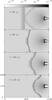 |
Fig. 4 Density xz-midplane stratifications for model M1b, which has only an EUV radiation field, from t = 80 yr (top) to t = 120 yr (bottom), showing the interaction between the stellar wind with the photoevaporated flow. The density scale (given by the top-bar) is in g cm-3. The coordinate axes are in AU. |
Our simulations include a flat, neutral disk, with a constant thickness H = 15.6 AU and an outer radius of 50 AU. The disk is positioned at distances of 0.02, 0.1 and 0.2 pc from the ionizing photon source. With this particular choice of parameters, we can in principle ensure that the photoevaporated flow of the nearest disk would be EUV-dominated, while for the more distant one, FUV-dominated. Using previous analytical calculations of Johnstone et al. (1998) and the disk radius given above, we can roughly estimate the minimum distance from the ionizing source in order to have an FUV-dominated flow as dmin ~ 0.1 pc. The disk radius that would support an FUV-dominated flow is, for d = 0.1 pc, rd ≈ 30 AU, and rd ≈ 120 AU for d = 0.2 pc (see Eqs. (15) and (16) in Johnstone et al. 1998). We choose to simulate disks at distances from the ionizing photon source that are i) at a distance that is suitable for an EUV-dominated flow (d = 0.02 pc), ii) close to the limiting cases for which we should expect an FUV dominated flow to occur (d = 0.1 pc, rd = 50 AU), and iii) FUV-dominated flow (d = 0.2 pc). In this last case, the disk radius rd = 50 AU is found to obey the rd ≲ 122 AU condition, and the system would develop an FUV-dominated flow. The only caveat is that, as pointed out by Johnstone et al. (1998), there are several sources of uncertainties in evaluating these (analytical) numbers.
The density of the disk is assumed to be constant in both the vertical and radial directions. We start the simulations assuming pressure equilibrium between the PDR region and the disk itself:  (3)where T2 and T3 are the PDR and disk temperatures (see Eq. (1)) and n0 is the number density at the base of the photoevaporated flow, which can be estimated as:
  (4)for a FUV dominated flow. Here, ND is the column density of the PDR attained for τFUV ~ 1 − 3, that is of the order of 1021 cm-2 (Johnstone et al. 1998). Using rd = 50 AU, we obtain n0 ~ 106 cm-3. We therefore set nd = 107 cm-3. For an EUV dominated flow, the density is found by equating the EUV flux to the recombinations in the ionized flow:
  (5)where αr = 2.6 × 10⁻¹³ cm3 s-1 is the recombination coefficient for Hydrogen at 104 K, d is the distance from the disk to the ionizing photon source, and SEUV = 7.2 × 1048 s-1 and rd = 50 AU in all of the models presented in this paper. We should note that the factor of 3 on the right hand side of Eq. (5) is a result of assuming a spherical divergence for the photoevaporated wind.
We then calculate the densities n0 for different distances and find n0 = (0.98 − 5.0) × 105 cm-3 for d = (0.1 − 0.02) pc. For all cases, we treat the disk as an infinite reservoir, since at each time step we reset its initial conditions, as described above.
We assume the presence of a 0.2 M⊙ star at the disk center and consider the gravitational force that it exerts on the flow (by including the appropriate source terms in the momentum and energy equations). A Keplerian rotation velocity law (consistent with the 0.2 M⊙ central star) is imposed on the disk material. The gravitational force is important as it inhibits the formation of a photoevaporated wind in the central regions of the disk. We expect a photoevaporated flow to start beyond the gravitational radius, which can be estimated as rg = GM ⋆ / a2, where a is the local sound speed. For FUV dominated flows, a ≃ 3 km s-1, so that rg = 2.9 × 1014 cm, or ≈ 20 AU. The inhibition of the photoevaporated wind in the central regions of the disk can be seen in our FUV dominated flow simulations (which have rg ≈ 20 AU), but not in our EUV dominated flow simulations (which have rg ≈ 2 AU, smaller than our numerical resolution). The size of the remnant disk, which is known to be typically smaller than the gravitational radius, will not be investigated in this work, since we are treating the disk as an infinite reservoir (Johnstone et al. 1998).
For some models, we add a plane-parallel wind (flowing parallel to the ionizing/dissociating external radiation field, with velocity vw = 100 km s-1 and with number density nw = 500 cm-3), which represents the wind from the O-type star. The wind velocity of θ1 Ori C is estimated to be of the order of 500 to 1650 km s-1 (Bally et al. 1998), or even larger (up to about 3600 km s-1, Walborn & Nichols 1994), which is by far larger than the adopted velocity here. On the other hand, the ram pressure estimated for both the stellar wind and the photoevaporated flow for proplyds in the Trapezium region is ~ 3 × 10⁻⁸ dyn cm-2 to 5 × 10⁻⁷ dyn cm-2 for the proplyds closer to θ1 Ori C (at distances ≃ 0.01 pc; see, e.g., Garcia-Arredondo et al. 2001). Therefore, our particular choice of parameters for the stellar wind give us a ram pressure comparable to that estimated for a group of proplyds in the Trapezium cluster. In particular, with the adopted parameters, we have Psw = 8.3 × 10⁻⁸ dyn cm-2.
 |
Fig. 5 Distances from the disk to the interaction region as a function of time are depicted for model M1b, which has only an EUV radiation field: dd − IR,c (full line) are the calculated distances, where stellar and the photoevaporated wind ram pressures match; dd − IR,m (dotted-line) are the distances as measured from the simulations (along the x-axis, with y = z = 4.9 × 1015 cm). The distances are in units of 1015 cm (left-axis). Also shown is the disk mass loss Ṁ (dashed-line), in units of 10-8 M⊙ yr-1 (right axis). The Ṁ has been calculated by computing the quantity ρA·v on the faces of a cube centered at the disk center, with a = 3rd. |
The initial setup of the simulations is shown in Fig. 2. The flat, dense structure with which we model the circumstellar disk is placed on the yz-plane, at x = 1 203 AU. The disk axis, which we define here as the axis perpendicular to the disk plane, and that contains the disk center at (x,y,z) = (1203, 334, 334) AU, coincides with the x-axis for an inclination angle θ = 0°. For larger inclination angles, the disk axis rotates clockwise, with respect to the x-axis, as depicted in Fig. 2. The remaining volume of the computational domain is filled with an ionized environment of uniform density na = 500 cm-3. All models except M1a have an initial wind of vw = 100 km s-1 and density nw = 500 cm-3, entering the computational domain through the x = 0 boundary. The ionizing/dissociating photon source is placed along the x-axis, outside the computational domain to the left.
In Table 1 we present all the relevant parameters used in our models: the dissociating photon rate, SFUV (in units of 1049 s-1; second column), the distance from the disk to the external star (in pc; third column), the inclination angle θ between the disk and the x axis (fourth column), the velocity of the wind from the external star (in km s-1; fifth column) and the temperature of the PDR region (in K; sixth column). All the models have an ionizing photon flux SEUV = 7.2 × 1048 s-1 (similar to the values used by Richling & Yorke 2000) and rd = 50 AU.
The simulations have been computed in a 5-level, binary adaptive grid with a maximum resolution (along the three axes) of 5.2 AU for all models. The computational domain has a size (xmax,ymax,zmax) = (1337, 668, 668) AU.
3. Results and discussion
In Fig. 3, we show the xz-midplane density stratifications (left) and Hα maps (right) for model M1a (top) and model M1b (bottom) at t = 2000 years. The models present only an EUV radiation field from the ionizing source (at a 0.1 pc distance from the disk). The difference between the two models is the presence of a stellar wind in model M1b, as described in Table 1. The disk axis has no inclination with respect to the direction of the impinging photons (i. e., θ = 0° see Fig. 2 and also Table 1).
The Hα emission in model M1a, is restricted to a region near the disk surface (and facing the ionizing source), and the edge of the shadow on the non-illuminated side of the disk. For model M1b, we have Hα emission close to the disk (with morphology and intensity similar to those seen in model M1a), and also fainter emission regions distributed along the interaction region between the stellar wind and the photoevaporated flow. It is known that some proplyds in Orion show faint Hα arcs facing θ1 Ori C (Bally et al. 1998), which correspond to the stellar wind/photoevaporated flow interaction emission found in our models.
 |
Fig. 6 Density xz-midplane stratifications (left) and Hα maps (right) for models M2a (top), M2b (middle) and M2c (bottom) at t = 2000 yr. The scales (given by the top bars) are in g cm-3 for the density (left), and normalized to one for the Hα maps (right). The coordinate axes are in AU. |
In Fig. 4 we show xz-midplane density maps for model M1b at t = 60, 80, 100 and 120 yr, in order to illustrate the initial evolution of such an interaction. At t = 60 yr, the stellar wind and the photoevaporated flow start to interact at x ≃ 668 AU. At later times, the interaction region moves towards the disk, and stabilizes around the position of the point of ram pressure balance between the stellar wind and the photoevaporated flow. We can also see this effect in Fig. 5, where we show the photoevaporated wind mass loss rate (Ṁ; dashed line), the distance from the disk to the interaction region i) as measured directly from the xz-midplane density maps (dd − IR,m; dotted-line) and ii) as calculated (dd − IR,c; full-line) by balancing the ram pressures from the stellar wind (Psw) and from the photoevaporated flow (Ppef). The expression for dd − IR,c, that takes into account the logarithmic outward acceleration expected for the photoevaporated wind is given by (see Henney et al. 1996):
![Mathematical equation: \begin{equation} \label{ramp} d_{{\rm{d-IR,c}}} \simeq R_0\cdot \bigg[1+ 4{\rm ln}\bigg( \frac{R_0}{r_{\rm d}} \bigg) \bigg]^{1/4}, \end{equation}](/articles/aa/full_html/2011/03/aa13342-09/aa13342-09-eq129.png) (6)where rd is the disk radius, and R0:
(6)where rd is the disk radius, and R0:  (7)In this equation, aII is the sound speed of the photoionized flow, and Psw is the ram pressure of the stellar wind, which is Psw = 8.3 × 10⁻⁸ dyn cm-2 for our chosen parameters (see Sect. 2). In Fig. 5, we see that both the measured and the calculated distances are comparable.
In Fig. 6, we show the xz-midplane density stratifications (left) and Hα maps (right) for models M2a (top), M2b (middle) and M2c (bottom), at t = 2000 years. The models have both EUV and FUV radiation fields (from the stellar source). The distance from the disk to the ionizing source is 0.2 pc, 0.1 pc and 0.02 pc for models M2a, M2b and M2c, respectively; see Table 1. The density of the disk is determined from Eqs. (3) and (4) for the FUV dominated models M2a and M2b, and Eqs. (3) and (5) for the EUV dominated model M2c. The disk axis is aligned with the x-direction (θ = 0° see Fig. 2 and also Table 1), and the stellar wind is present in the three models.
 |
Fig. 7 Density xz-midplane stratifications superimposed on velocity field vectors (left panels) and an xz-map of the Mach number (right panels), M = v / a (a is the local sound speed) for models M2a (top) and M2b (bottom), at t = 200 yr. The snapshots are a closer view of the star-disk system being photoevaporated. The distance (in AU) to the origin of the coordinate system is depicted for the x and z axes in the left panels. The right-hand side bars on each panel indicate the density scale (in g cm-3; left panels) and the Mach number (right panels). The labels in the top-rigth panel indicates the region where we have a supersonic outflow (1 and 3), a subsonic outflow (2), and a subsonic inflow (4). We also note that region (1) is neutral, at a temperature T2 = 103 K, whereas (3) is ionized, at a temperature T1 = 104 K. |
We see that a high density region shrouds the disk in models M2a and M2b. This region is related to the photodissociation region expected from the analytical models of Johnstone et al. (1998) and Störzer & Hollenbach (1999). It has a temperature T2 ≃ 1000 K (see Eq. (1) and Table 1). This region is composed of C ii and H i. We also note that the environment (the left part of the computational domain) and the photoevaporated wind outside the PDR have a temperature of about 104 K, indicating that they are photoionized. The photodissociation region separates the disk from the ionized photoevaporated wind. In model M2c (in which the disk is at 0.02 pc from the ionizing photon source) the photodissociation region is limited to a thin shell in contact with the surface of the disk.
The ionization front radius (as defined in Fig. 2) is found to grow from rIF = 2.4rd = 120 AU at t = 200 yr to rIF = 3.8rd = 190 AU at t = 2000 yr for model M2a, while for model M2b, rIF = 1.6rd = 80 AU (constant throughout the simulation). In models M2a and M2b, the outer radius of the photodissociation region (rw, defined in Fig. 2) grows with time. This lateral expansion occurs at a velocity of ≈ 0.1 km s-1, at ~ 1 / 10 of the ~ 1 km s-1 outwards flow velocity of the gas within the photodissociation region. This indicates that the ionization front in these models is pressure confined by the base of the photoevaporated flow. The ratio between the cross section radius rw and the axial standoff distance rIF (see Fig. 2) has values rw / rIF = 1.4 and 1.9 for models M2a and M2b (at t = 2000 yr), respectively. Interestingly, Johnstone et al. (1998) predict rw = 1.3rIF from their simplified, analytic model. Models M2a and M2b have detached, almost hemispherical ionization fronts. On the other hand, in model M2c the ionization front lies very close to the surface of the disk (with just one pixel of separation between them). It is interesting to note that observations of proplyd 170 − 337 (Johnstone et al. 1998), that is situated at 0.1 pc from θ1 Ori, show that its IF radius is approximately 80 AU. From the analytical calculations of Johnstone et al. (1998) for FUV dominated flows,  , where rIF14 is the radius of the IF in units of 1014 cm, d17 is the distance from the source in units of 1017 cm, S49 is the ionizing photon rate in units of 1049 s-1, fr is the fraction of EUV photons absorbed by recombination in the ionized region of the flow, and ϵ is a dimensionless parameter of order unity (see Johnstone et al. 1998). Taking (ϵ2 / frS49) = 16 (Johnstone et al. 1998), and d17 = 3.08, we obtain rIF ≃ 100 AU, which is consistent with the values obtained from models M2a and M2b.
In Fig. 7 we show the velocity field in a region close to the accretion disk superimposed on density (left panels) and Mach number maps (right panels), M = v / a, where a is the local sound speed and v is the local velocity of the gas, for models M2a (top panels) and M2b (bottom panels), at t = 200 yr. From Fig. 7, we see that the photoevaporated flow has four different dynamical regimes, indicated in the top-right panel of Fig. 7 by the labels 1 to 4, which refer to: 1) a supersonic neutral outflow; 2) a subsonic, neutral outflow, both of them inside the PDR region and separated by a shock; 3) a supersonic, ionized outflow outside the PDR region and 4) a subsonic, neutral inflow, localized around the disk center (at r ≲ rg).
 |
Fig. 8 Density xz-midplane stratifications (left) and Hα maps (right) obtained from models M3a (top) and M3b (bottom) for t = 2000 yr. The scales (given by the top bars) are in g cm-3 for the density (left), and normalized to one for the Hα maps (right). The coordinate axes are in AU. The distance between the ionized photon source and the disk is d = 0.2 pc and d = 0.1 pc for models M3a and M3b, respectively. In both cases, θ = 45° (see Fig. 2). |
 |
Fig. 9 Density xz-midplane stratifications (left) and Hα maps (right) obtained from models M4a (top) and M4b (bottom) for t = 2000 yr. The scales (given by the top bars) are in g cm-3 for the density (left), and normalized to one for the Hα maps (right). The coordinate axes are in AU. |
 |
Fig. 10 Density xz-midplane stratifications superimposed on velocity field vectors for models M3a (top-left), M3b (top-right), M4a (bottom-left) and M4b (bottom-right), at t = 2000 yr. The distance to the origin of the coordinate system, in AU, is depicted for the x and z axes. The right-hand side bars indicate the density scale (in g cm-3). |
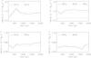 |
Fig. 11 The mass loss rate as a function of time for models M1a and M1b (top-left panel), M2a, M2b and M2c (top-right panel), M3a and M3b (bottom-left panel) and M4a and M4b (bottom-right panel). The caption on the top of each diagram indicates the model that a given curve type represents. The mass loss rate is in units of 10-7 M⊙ yr-1 for models M2, M3 and M4 and in units of 10-8 M⊙ yr-1 for models M1. |
In Fig. 8 we show the xz-midplane density stratifications (left) and Hα maps (right) for models M3a (top) and M3b (bottom panels) at t = 2000 yr. The models have an EUV+FUV radiation field from the ionizing source, that is located at 0.2 pc (M3a) and 0.1 pc (M3b) distance from the disk. In both cases, the disks have a 45° of inclination with respect to the direction of the impinging photons (θ = 45° see Fig. 2 and Table 1). In Fig. 9 we present the same results, but for models M4a and M4b (with θ = 75°). As can be seen in Table 1, models M2a, M3a and M4a differ only by the values of the disk inclination. The same is true for the set of models M2b, M3b and M4b.
In the inclined disk models (models M3a, M3b, M4a and M4b, see Figs. 8, 9) the internal structure of the PDR region is the same as in the M2a and M2b models (with θ = 0°, see Fig. 7 and Table 1). There is a neutral supersonic outflow (with M ≈ 2 in all models) near the illuminated surface of the disk. For inner disk radial distances (from the disk axis), there is a gas inflow. In Fig. 10 we show velocity vectors superimposed on density maps for models M3a (top-left), M3b (top-right), M4a (bottom-left) and M4b (bottom-right). As in the M2a and M2b models, we again have an internal shock that separates the supersonic from the subsonic neutral flows, inside the PDR. Outside this internal shock we have the outer edge of the PDR region, that separates the subsonic, neutral flow from the external, ionized supersonic flow. These structures are characteristic of an FUV dominated flow, as discussed previously.
The Hα emission in the region close to the ionization front of models M3 and M4 (Figs. 8 and 9) has a general morphological resemblance to the Hα morphology of the “face-on” models (M2, see Fig. 6). However, the Hα maps of the inclined disk models show clear side-to-side asymmetries, which are more pronounced for the models with θ = 45° (M3a, b, see Table 1 and Fig. 8) than for the ones with θ = 75° (M4a, b, see Fig. 9).
From the t = 2000 yr time-frames of models M3 and M4 (see Figs. 8 and 9), we have calculated the axial stand-off distance (rIF) and width of the cross section presented by the ionization front (rw, see Fig. 2). We obtain the following results:
- –
M3a: rIF = 3.6rd = 180 AU; rw = 4.4rd = 220 AU;
M3b: rIF = 2.0rd = 100 AU; rw = 2.4rd = 120 AU;
M4a: rIF = 2.8rd = 140 AU; rw = 3.7rd = 185 AU;
M4b: rIF = 1.9rd = 95 AU; rw = 2.1rd = 105 AU,
In Fig. 11 we present the mass loss rate as a function of time, for all the simulated models except model M2d. The mass loss rate for models M1a and M1b (without an FUV radiation field; see Table 1) shows a small time variability (as mentioned above), but is almost independent of the presence of the stellar wind. Also, the mass loss rate has approximately the same value even if the distance from the disk to the ionizing photon source changes by a factor of two, even for the are FUV dominated models, as is the case for those with a given inclination angle (with respect to the ionizing photon source) as M2a and M2b (θ = 0°), M3a and M3b (θ = 45°), and M4a and M4b (θ = 75°). This is due to our simplified model, in which the PDR temperature is assumed to be position independent and with the same value for all models. Looking at a series of models with increasing values of the inclination angle θ (e.g., models M2a, M3a and M4a, which otherwise have identical paramenters, see Table 1), we see that the mass loss rate as a monotonically decreasing function of θ. This result is to be expected, given the lower effective cross sections (to the impinging UEV/FUV radiation field) presented by the disk for increasing inclination angles. In particular, if we take the mean value of Ṁ for models M2a and M2b (with θ = 0), for models M3a and M3b (with θ = 45°) and for models M4a and M4b (with θ = 75°), we find ṀM2 = 1.4 × 10⁻⁷ M⊙ yr-1, ṀM3 = 6.2 × 10⁻⁸ M⊙ yr-1ṀM4 = 4.8 × 10⁻⁸ M⊙ yr-1, which implies ṀM3 ≃ 0.4ṀM2 and ṀM4 ≃ 0.3ṀM2.
In Fig. 12, we show the xz-midplane density stratifications (left) and Hα maps (right) for model M2d at t = 200 yr. This model has the same parameters as the M2b model (θ = 0°, d = 0.1 pc; see Table 1) but a different PDR temperature T2 = 3000 K (see Eq. (1)). The ionization front radius is larger, by a factor of ≃ 3, for the model M2d when compared with those with T2 = 1000 K. The mass loss rate is ≈ 5 × 10⁻⁷ M⊙ yr-1 for M2d (about 3.5ṀM2). We have run equivalent simulations for models M3b and M4b, that is, a model with θ = 45° and d = 0.1 pc, but with T2 = 3000 K, and a model with θ = 75° and d = 0.1 pc, but with T2 = 3000 K. For these models (not shown here), we found the same trend of larger mass loss rates and ionization front standoff distances for larger values of T2.
4. Conclusions
This work describes the first fully three-dimensional numerical gasdynamic simulations of the photoevaporation of neutral disks, subject to an interaction with the FUV/EUV photon flux and the wind from an external O star.
With this initial setup, we study the time-evolution of the photoevaporated flow. We have calculated models in the EUV dominated regime, in which one obtains an ionization front (IF) close to the surface of the disk, and a photodissociation region (PDR) not resolved by our numerical scheme between the surface of the disk and the IF, and in the FUV dominated regime, in which a PDR (well resolved in our numerical simulations) is formed between the surface of the disk and the IF. Both EUV and FUV dominated models develop an interaction region between the photoevaporated wind and the wind from the hot star. In some cases, this interaction region lies within our computational domain. For these cases, the interaction region lies close to the position of stellar wind/photoevaporated flow ram pressure balance.
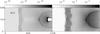 |
Fig. 12 Density xz-midplane stratification (left) and Hα map (right) for model M2d at t = 200 yr. The temperature of the PDR region in this model is T2 = 3000 K. The scales (given by the top bars) are in g cm-3 for the density (left), and normalized to one for the Hα maps (right). The coordinate axes are in AU. |
We have simulated models of disks with different inclinations with respect to the direction of the impinging EUV and FUV photon fluxes, and at different distances from the ionizing photon sources ranging from 0.02 pc to 0.2 pc. The model at a distance of 0.02 pc from the O-star is clearly EUV dominated, since the IF is just above the disk surface. Models at distances from 0.1 pc to 0.2 pc show detached PDRs. These PDRs show structures, such as the presence of a neutral supersonic flow near the disk and, farther out but before reaching the IF, a subsonic neutral flow, that are consistent with the main features predicted by Johnstone et al. (1998) for a FUV-dominated flow. We note that these structures occur in our simulations even for the inclined disk models. The typical size of the IF was found to be in agreement with analytical results. In particular, the limits predicted by Johnstone et al. (1998) for the ionization front radius, 2.5rd ≲ rIF ≲ 4rd, were recovered in most of the models, with or without disk inclination.
We found that, for a given inclination of the disk, the mass loss rate seems to be independent of the distance to the FUV/EUV photon source (for the FUV-dominated flows). In our simulations this is due to the constancy of the PDR temperature. For higher disk inclinations, we obtain smaller mass loss rates, which is a direct result of the smaller effective cross section presented by the disk to the impinging FUV/EUV photon flux. Taking the mean values of the mass loss rate from our simulations, we obtain ṀM2 = 1.4 × 10⁻⁷ M⊙ yr-1, ṀM3 = 6.2 × 10⁻⁸ M⊙ yr-1ṀM4 = 4.8 × 10⁻⁸ M⊙ yr-1, for models with θ = 0°, θ = 45° and θ = 75°, respectively. These values are surprisingly similar, in spite of the very different inclination angles used in the simulations.
Our models predict Hα emission maps with moderate side-to-side asymmetries, which directly result from the misalignment of the axis of the accretion disk with respect to the direction to the photoionizing source. Asymmetries are seen both in the emission associated with the IF and in the emission of the photoevaporated wind/expanding H II region interaction working surface. It is clear that asymmetries in these two structures are indeed observed in many of the Orion proplyds (Bally et al. 2000). A detailed attempt to model a specific, asymmetrical proplyd with a 3D photoionizing disk simulation will be presented in a future paper.
Acknowledgments
We thanks the anonymous referee for his/her comments and suggestions, which contributes to improve the quality of the manuscript. M.J.V. would like to thanks FAPESB for partial financial support (PPP project 7606/2006). A.H.C. wish to thank the Brazilian agency CNPq for partial financial support (projects 307036/2009-0 and 471254/2008-8), and also PROPP-UESC (projects 635 and 802). A.R. acknowledges support from the CONACyT grants 61547, 101356, and 101975. We thank A. Esquivel for sharing with us a set of IDL routines for plotting the YGUAZU-a output.
References
- Bally, J., Shuterland, R. S., Devine, D., Johnstone, D. 1998, AJ, 116, 293 [NASA ADS] [CrossRef] [Google Scholar]
- Bally, J., O’Dell, C. R., & McCaughrean, M. J. 2000, AJ, 119, 2919 [NASA ADS] [CrossRef] [Google Scholar]
- Cardelli, J. A., Clayton, G. C., Mathis, J. S. 1988, ApJ, 329, L33 [NASA ADS] [CrossRef] [Google Scholar]
- Cerqueira, A. H., Velázquez, P. F., Raga, A. C., Vasconcelos, M. J., & De Colle, F. 2006a, A&A, 448, 231 [NASA ADS] [CrossRef] [EDP Sciences] [Google Scholar]
- Cerqueira, A. H., Cantó, J., Raga, A. C., & Vasconcelos, M. J. 2006b, Rev. Mexicana Astron. Astrofis., 42, 203 [Google Scholar]
- Churchwell, E., Felli, M., Wood, D. O. S., & Massi, M. 1987, ApJ, 321, 516 [NASA ADS] [CrossRef] [Google Scholar]
- García-Arredondo, F., Henney, W. J., & Arthur, S. J. 2001, ApJ, 561, 830 [NASA ADS] [CrossRef] [Google Scholar]
- González, R. F., de Gouveia Dal Pino, E. M., Raga, A. C., & Velázquez, P. F. 2004, ApJ, 616, 976 [Google Scholar]
- Henney, W. J., Raga, A. C., Lizano, S., & Curiel, S. 1996, ApJ, 465, 216 [NASA ADS] [CrossRef] [Google Scholar]
- Henney, W. J., O’Dell, C. R., Meaburn, J., Garrington, S. T., & Lopez, J. A. 2002, ApJ, 566, 315 [NASA ADS] [CrossRef] [Google Scholar]
- Johnstone, D., Hollenbach, D., & Bally, J., 1998, ApJ, 499, 758 [NASA ADS] [CrossRef] [Google Scholar]
- Laques, P., & Vidal, J. L. 1979, A&A, 73, 97 [NASA ADS] [Google Scholar]
- Lefloch, B., & Lazareff, B. 1994, A&A, 289, 559 [NASA ADS] [Google Scholar]
- Masciadri, E., Velázquez, P. F., Raga, A. C., Cantó, J., & Noriega-Crespo, A. 2002, ApJ, 573, 260 [NASA ADS] [CrossRef] [Google Scholar]
- O’Dell, C. R., & Wen, Z. 1994, ApJ, 436, 194 [NASA ADS] [CrossRef] [Google Scholar]
- O’Dell, C. R., & Wong, K. 1996, AJ, 111,846 [NASA ADS] [CrossRef] [Google Scholar]
- O’Dell, C. R., Wen, Z., & Hu, X. 1993, ApJ, 410, 696 [CrossRef] [Google Scholar]
- Raga, A. C., Navarro-González, R., & Villagran-Muniz, M. 2000, Rev. Mexicana Astron. Astrofis., 36, 67 [Google Scholar]
- Raga, A. C., Sobral, H., Villagrán-Muniz, M., Navarro-González, R., & Masciadri, E. 2001, MNRAS, 324, 206 [NASA ADS] [CrossRef] [Google Scholar]
- Raga, A. C., de Gouveia Dal Pino, E. M., Noriega-Crespo, A., Mininni, P. D., & Velázquez, P. F. 2002, A&A, 392, 267 [NASA ADS] [CrossRef] [EDP Sciences] [Google Scholar]
- Richling, S., & Yorke, H. W. 2000, ApJ, 539, 258 [NASA ADS] [CrossRef] [Google Scholar]
- Sobral, H., Villagrán-Muniz, M., Navarro-González, R., & Raga, A. C. 2000, Apl. Phys. Lett., 77, 3158 [Google Scholar]
- Störzer, H., & Hollenbach, D. 1999, ApJ, 515, 669 [CrossRef] [Google Scholar]
- Takami, M., Usuda, T., Sugai, H., et al. 2002, ApJ, 566, 910 [NASA ADS] [CrossRef] [Google Scholar]
- Van Leer, B. 1982, ICASE Report, 82 [Google Scholar]
- Vasconcelos, M. J., Cerqueira, A. H., Plana, H., Raga, A. C., & Morrisset, C. 2005, AJ, 130, 1707 [NASA ADS] [CrossRef] [Google Scholar]
- Velázquez, P. F., de la Fuente, E., Rosado, M., & Raga, A. C. 2001a, A&A, 377, 1136 [NASA ADS] [CrossRef] [EDP Sciences] [Google Scholar]
- Velázquez, P. F., Sobral, H., Raga, A. C., Villagrán-Muniz, M., & Navarro-González, R. 2001b, Rev. Mexicana Astron. Astrofis., 37, 87 [Google Scholar]
- Velázquez, P. F., Martinell, J. J., Raga, A. C., & Giacani, E. B. 2004, ApJ, 601, 885 [NASA ADS] [CrossRef] [Google Scholar]
- Yorke, H. W., & Bodenheimer, P. 1999, ApJ, 525 [Google Scholar]
- Walborn, N. R., & Nichols, J. S. 1994, ApJ, 425, L29 [NASA ADS] [CrossRef] [Google Scholar]
All Tables
All Figures
|
Fig. 1 A cartoon of a star-disk system being photoevaporated by the UV radiation field from an O type star. The major features are highlighted: the proplyd head and tail which traces the ionization front from the direct ionization field coming from the O-star and from the diffuse radiative field, respectively, and the interaction region between the photoevaporated flow and the wind from the O-star. |
| In the text | |
|
Fig. 2 Schematic view of the initial setup of the simulations. The cartoon shows also the distance from the disk to the ionization front, rIF, and the definition of the width of the ionized structure, rw. We follow the notation of Johnstone et al. (1998) (see Fig. 7 in that paper). |
| In the text | |
|
Fig. 3 Density xz-midplane stratifications (left) and Hα maps (right) obtained from models M1a (top) and M1b (bottom) which has only an EUV radiation field for t = 2000 yr. The scales (given by the top-bars) are in g cm-3 for the density (left), and normalized to one for the Hα maps (right). The coordinate axes are in AU. |
| In the text | |
|
Fig. 4 Density xz-midplane stratifications for model M1b, which has only an EUV radiation field, from t = 80 yr (top) to t = 120 yr (bottom), showing the interaction between the stellar wind with the photoevaporated flow. The density scale (given by the top-bar) is in g cm-3. The coordinate axes are in AU. |
| In the text | |
|
Fig. 5 Distances from the disk to the interaction region as a function of time are depicted for model M1b, which has only an EUV radiation field: dd − IR,c (full line) are the calculated distances, where stellar and the photoevaporated wind ram pressures match; dd − IR,m (dotted-line) are the distances as measured from the simulations (along the x-axis, with y = z = 4.9 × 1015 cm). The distances are in units of 1015 cm (left-axis). Also shown is the disk mass loss Ṁ (dashed-line), in units of 10-8 M⊙ yr-1 (right axis). The Ṁ has been calculated by computing the quantity ρA·v on the faces of a cube centered at the disk center, with a = 3rd. |
| In the text | |
|
Fig. 6 Density xz-midplane stratifications (left) and Hα maps (right) for models M2a (top), M2b (middle) and M2c (bottom) at t = 2000 yr. The scales (given by the top bars) are in g cm-3 for the density (left), and normalized to one for the Hα maps (right). The coordinate axes are in AU. |
| In the text | |
|
Fig. 7 Density xz-midplane stratifications superimposed on velocity field vectors (left panels) and an xz-map of the Mach number (right panels), M = v / a (a is the local sound speed) for models M2a (top) and M2b (bottom), at t = 200 yr. The snapshots are a closer view of the star-disk system being photoevaporated. The distance (in AU) to the origin of the coordinate system is depicted for the x and z axes in the left panels. The right-hand side bars on each panel indicate the density scale (in g cm-3; left panels) and the Mach number (right panels). The labels in the top-rigth panel indicates the region where we have a supersonic outflow (1 and 3), a subsonic outflow (2), and a subsonic inflow (4). We also note that region (1) is neutral, at a temperature T2 = 103 K, whereas (3) is ionized, at a temperature T1 = 104 K. |
| In the text | |
|
Fig. 8 Density xz-midplane stratifications (left) and Hα maps (right) obtained from models M3a (top) and M3b (bottom) for t = 2000 yr. The scales (given by the top bars) are in g cm-3 for the density (left), and normalized to one for the Hα maps (right). The coordinate axes are in AU. The distance between the ionized photon source and the disk is d = 0.2 pc and d = 0.1 pc for models M3a and M3b, respectively. In both cases, θ = 45° (see Fig. 2). |
| In the text | |
|
Fig. 9 Density xz-midplane stratifications (left) and Hα maps (right) obtained from models M4a (top) and M4b (bottom) for t = 2000 yr. The scales (given by the top bars) are in g cm-3 for the density (left), and normalized to one for the Hα maps (right). The coordinate axes are in AU. |
| In the text | |
|
Fig. 10 Density xz-midplane stratifications superimposed on velocity field vectors for models M3a (top-left), M3b (top-right), M4a (bottom-left) and M4b (bottom-right), at t = 2000 yr. The distance to the origin of the coordinate system, in AU, is depicted for the x and z axes. The right-hand side bars indicate the density scale (in g cm-3). |
| In the text | |
|
Fig. 11 The mass loss rate as a function of time for models M1a and M1b (top-left panel), M2a, M2b and M2c (top-right panel), M3a and M3b (bottom-left panel) and M4a and M4b (bottom-right panel). The caption on the top of each diagram indicates the model that a given curve type represents. The mass loss rate is in units of 10-7 M⊙ yr-1 for models M2, M3 and M4 and in units of 10-8 M⊙ yr-1 for models M1. |
| In the text | |
|
Fig. 12 Density xz-midplane stratification (left) and Hα map (right) for model M2d at t = 200 yr. The temperature of the PDR region in this model is T2 = 3000 K. The scales (given by the top bars) are in g cm-3 for the density (left), and normalized to one for the Hα maps (right). The coordinate axes are in AU. |
| In the text | |
Current usage metrics show cumulative count of Article Views (full-text article views including HTML views, PDF and ePub downloads, according to the available data) and Abstracts Views on Vision4Press platform.
Data correspond to usage on the plateform after 2015. The current usage metrics is available 48-96 hours after online publication and is updated daily on week days.
Initial download of the metrics may take a while.