| Issue |
A&A
Volume 526, February 2011
|
|
|---|---|---|
| Article Number | A25 | |
| Number of page(s) | 16 | |
| Section | Celestial mechanics and astrometry | |
| DOI | https://doi.org/10.1051/0004-6361/201015500 | |
| Published online | 15 December 2010 | |
Astrophotometric variability of CFHT-LS Deep 2 QSOs⋆,⋆⋆
1
Observatoire de Paris, Systèmes de Référence Temps Espace (SYRTE),
CNRS/UMR8630, Paris
France
e-mail: Francois.Taris@obspm.fr
2
Observatório Nacional/MCT, Rio de Janeiro,
Brasil
3
Observatório do Valongo/UFRJ, Rio de Janeiro,
Brasil
4
Osservatorio Astronomico di Torino/INAF,
Torino,
Italy
5 CICGE-Fac. Sciences Univ. Porto, Porto, Portugal
Received: 29 July 2010
Accepted: 12 October 2010
Context. The current conventional realization of the ICRS (International Celestial Reference System) is, in the radio wavelength, the International Celestial Reference Frame 2 (ICRF2). The individual positions of the defining sources have been found to have accuracies better than 1 milliarcsecond (mas). In 2012, the European astrometric satellite Gaia will be launched. This mission will provide an astrometric catalog of an estimated number of 500 000 QSOs. The uncertainty in the coordinates is anticipated to be 200 microarcsecond (μas) for the magnitude = 20. If this were achieved, the ICRF and the Gaia related reference frame could be related with a μas accuracy.
Aims. The goal of this work is both to measure the photometric variability of a set of quasars in a given field, and search wether this variability can be related to an astrometric instability characterized by a motion of the quasar photocenter. If this correlation existed for some given QSO, then it would be inadequate to materialize the Gaia extragalactic reference frame at the level of confidence required, i.e. the sub-milliarcsecond one. This should be an important result in the scope of the Gaia mission.
Methods. We use QSO CCD images obtained over 4.5 years with the Canada France Hawaï Telescope (CFHT) in the framework of the CFHT-Legacy Survey (CFHT-LS). The pictures were analysed with both the SExtractor software and customised codes to perform a photometric calibration together with an astrometric one. A total of 41 QSOs in the Deep 2 field were analysed. Magnitude variations during more than 50 months are given at three different bandwiths G, R, and I. Among the set above, 5 quasars were chosen to test the ties between the postion of their centroid and their magnitude variations. For one of these 5 QSOs, the proximity of a neighbouring star allows the comparison between the PSFs.
Results. We clearly show significant photometric variations reaching sometimes more than one magnitude, for a good proportion of the 41 quasars in our sample. We show that these variations often occur within a few months, and that the correlation between the photometric curves in the three bands, G, R and I is obvious. As a second important result, we show that with a reasonably high probability, photometric variations for one quasar in our sample are accompagnied by substantial modification of its PSF.
Key words: reference systems / astrometry / quasars: general
This paper is dedicated to the memory of Anne-Marie Gontier (1966-2010). A.-M. Gontier was an expert in the field of Earth rotation, reference systems and the modeling, analysis, and processing of VLBI observations for astrometric and geodetic applications.
Figures 4–14 are only available in electronic form at http://www.aanda.org
© ESO, 2010
1. Introduction
Quasars have long been found to exhibit changes in their optical fluxes of between a tenth of a magnitude to a number of magnitudes. Measurable variations can occur within a few hours (microvariability, intra-night variabilty) or with periods of days to weeks (short-term variability). Long-term variability (periods up to several years) are also common (Smith et al. 1993). The timescale of the optical flux variations can thus vary from hours to years (Gupta et al. 2005).
Several astrophysical mechanisms have been invoked to explain the variability of quasars (Rabbette et al. 1998; Zackrisson et al. 2003; Hawkins 2002). The most popular are instabilities in the accretion disc around the central black hole, supernova bursts, jet instabilities, and gravitational microlensing by a population of small compact bodies along the line of sight.
One can postulate that a rapid flux variation is generated by a small emitting region (near the black hole) and that a longer-term flux variation is produced by a more extended region (core of the host galaxy, dust torus). In this case, these two regions (confined and extended) correspond, respectively (for a redshift near z = 1), to angular distances in the sky of between 1 μas and 100 μas.
In 2020, two reference catalogues will be available: (i) the current or an extended version of the second release of the International Celestial Reference Frame (ICRF2, see Sect. 3.2) at radio wavelengths; and (ii) the GAIA optical extragalactic reference frame. Both catalogues will have positional uncertainties smaller than 100 μas.
The ICRF2 axis stability depends on the positional stability of the defining sources. A number of studies have shown that using sources exhibiting significant apparent motion of the radio center to define the axes contaminates other very long baseline interferometry (VLBI) products such as Earth orientation parameters or station and source coordinates (see, e.g., Gontier et al. 2001; Feissel 2003; Feissel et al. 2006; Lambert et al. 2008; Lambert & Gontier 2009). At a wavelength of 3.6 cm, radio center displacements are due to flux variations or jets (e.g., Fey et al. 1997). This also applies to the optical domain: the accuracy of a quasar’s coordinates may be affected by intrinsic displacements of its centroid, which are potentially associated with photometric variations. In these cases, quasars would be poorly apt to materialize the GAIA extragalactic reference frame at the required level of precision.
Starting from these considarations, the goal of our work has been to study both the magnitude variations of quasars and the potentially correlated motions of their centroids. We used QSOs images obtained during a 4.5 year observational campaign with the Canada France Hawaï Telescope (CFHT) in the framework of the CFHT-Legacy Survey (CFHT-LS).
The CFHT-LS is a large project joining Canada, France, and the University of Hawaii. It consists of a survey of some fields in the sky with different scientific goals. It is based on observational data from the 3.6 m Canada-France-Hawaii telescope1, including pre-processing and calibration. A CCD camera (MEGACAM, Fig. 15) is located at the heart of the prime focus upper end of the telescope. It is composed of 36 (+4) CCD’s each of them with 2048 × 4612 pixels (378 Megapixels). Each pixel is 13.5 micrometers and the pixel scale is 0.185 arsecond/pixel. The field of view is 1 square degree and each image represents approximately 770 Megabytes2. The Terapix centre based at the Institut d’Astrophysique de Paris (IAP) is in charge of data resampling and stacking, optimization of astrometric and photometric calibration, and source catalog generation. SExtractor (Bertin et al. 1996) is a program that compiles a catalogue of objects from an astronomical image. Although it is designed in particular for the analysis of large-scale galaxy survey data, it is also suitable for moderately crowded star fields3. Sextractor was used in that study together with home-made software. The last component of the CFHT-LS is the Canadian Astronomy Data Centre (CADC)4 for all activities related to the archiving and release of the various data products to the scientific community.
In the next section, we present the main characteristics of catalogues and reference frames discussed in this work. In another section, the luminosity curves of the Deep 2 field quasars are presented together with a study of their position through the use of their PSF. The last section presents the consequences of our study as well as the work currently in progress to complete the results shown in this paper.
2. Reference systems
Our present study of quasars is from an astrometric point of view. We briefly review state-of-the-art projects to construct celestial reference frames from these objects.
2.1. General comments
The current conventional realization of the ICRS (International Celestial Reference System) is the second version of the International Celestial Reference Frame (ICRF) called ICRF2. In the optical domain, the Hipparcos Catalogue is the current international conventional realization but in the future (around 2020) the Gaia catalogue should be the basis of the optical realization of the ICRS. The link between these reference frames, in the radio and in the optical domain, is of course of primary significance. In this section, we present, in a didactic way, all of these fundamental concepts.
2.2. Radio reference frame: the ICRF2
At the 2009 XXVIIth IAU General Assembly at Rio, Brazil, the astronomical community adopted the second release of the International Celestial Reference Frame (ICRF2; Fey et al. 2009) as the new fundamental astrometric realization of the ICRS. From 1 January 2010, the ICRF2 replaces the ICRF (Ma et al. 1998) and its most recent extension (Fey et al. 2004).
The construction of the ICRF2 used almost 30 years of geodetic very long baseline interferometry (VLBI) observations at 3.6 cm and 13 cm wavelengths. The ICRF2 catalogue contains positions of 3414 compact radio sources. The formal errors σ in source coordinates increased according to  where σ0 is a noise floor set to 40 μas. The median error in the position of sources observed in more than two sessions is 175 μas. The frame axes are defined by the coordinates of 295 “defining” sources with a stability of ~10 μas. The defining sources were chosen on the basis of their high positional stability and low structure index. A subset of 138 defining sources was used to align the ICRF2 catalogue onto the ICRS.
The ICRF2 currently represents the most accurate realization of the celestial system with respect to which the position of any object in the celestial sphere should be measured. We note that the ICRF is epochless and independent of the dynamical frame (ecliptic) and reference point (equinox), but is consistent with previous realizations of the ICRS, including the FK5 J2000.0 optical system.
2.3. Optical reference frames
2.3.1. The Hipparcos catalogue
In 1997, during the IAU General Assembly at Kyoto, it was decided that the Hipparcos catalogue would be the primary realization of the ICRS at optical wavelengths (resolution B2). The Hipparcos Catalogue provides the equatorial coordinates of about 118 000 stars in the ICRS at epoch 1991.25 along with their proper motions, their parallaxes and their magnitudes in the wide Hipparcos band system. The astrometric data concerns only 117 955 stars. The median uncertainty for bright stars (Hipparcos wide-band magnitude brighter than 9) are ±0.77 mas and ±0.64 mas in right ascension and declination, respectively. In addition, the median uncertainties in annual proper motions are ±0.88 and ±0.74 mas/yr, respectively.
The alignment of the Hipparcos Catalogue to the ICRF was realized with a standard error of ±0.6 mas in the orientation at epoch (1991.25) and ±0.25 mas/year in the spin (Kovalevsky et al. 1997). This was obtained by comparing positions and proper motions of Hipparcos stars with the same subset determined with respect to the ICRF and, for the spin, to galaxies at optical wavelengths.
2.3.2. Toward the Gaia extragalactic reference frame
The European astrometric space mission Gaia will be launched in 2012. It will provide positions and proper motions of around one billion of stars and about 500 000 QSOs with unprecedented uncertainty between the 6th and the 20th magnitude (Lindegren 2009). The predicted accuracy is a few hundred of μas at 20th magnitude. To prepare the future Gaia extragalactic reference frame, a clean sample of at least 10 000 QSOs must be implemented (Gaia initial quasar list). This work is being performed in the framework of the Gaia workpackage GWP-S-335-13000 with the aim of giving an initial QSO catalogue (A. Andrei).
Two catalogues are at the basis of this work, the LQAC (Souchay et al. 2009) and the LQRF (Andrei et al. 2009).
The LQAC contains 113 666 quasars. It is a compilation of the 12 largest quasar catalogues (four from radio VLBI programs, eight from optical surveys). Information about u, b, v, g, r, i, z, J, K photometry as well as redshift and radio fluxes at 1.4 GHz, 2.3 GHz, 5.0 GHz, 8.4 GHz, and 24 GHz are given when available. A small proportion of the remaining objects not present in the 12 catalogues but included in the Véron-Cetty and Véron quasar catalogues (Véron-Cetty & Véron 2006) are added to the compilation.
The LQRF contains 100 165 quasars well represented across the sky, from −83.5° to +88.5° in declination. The average distance between adjacent elements is 10 arcmin. The global alignment with the ICRF is 1.5 mas, and the individual position accuracies are represented by a Poisson distribution peaking at 139 mas in right ascension and 130 mas in declination. The LQRF contains equatorial coordinates at epoch J2000.0, and is completed by redshift and photometric information from the LQAC.
2.4. The link between ICRF2 and the Gaia extragalactic reference frame
Relating the ICRF2 to the Gaia extragalactic reference frame will be a very important task in the near future and some work is currently underway to achieve this.
Bourda et al. (2008) evaluated the suitability of the current individual ICRF-Ext2 (the ICRF catalogue that preceded the ICRF2) extragalactic radio sources for the alignment with the future Gaia frame. They identify 243 candidates among the ICRF-Ext2 sources used to align with the Gaia frame, with an optical counterpart brighter than the apparent magnitude V = 18. Among these 243 candidates, only 70 have data of excellent or good astrometric quality (i.e., an X-band structure index value of either 1 or 2) for determining the Gaia link with the highest accuracy. Nevertheless, this index value is perhaps not well suited to determining the best sources in the optical domain in the sense that several sources given by these authors are not point-like sources (for example NGC 3031 or Messier81, MARK421, NGC 4374 or Messier84).
An investigation of the correlation between long-term optical variability and what is dubbed the random walk of the astrometric centroid of QSOs is being pursued at the ESO Max Planck 2.2 m telescope in Chile (Andrei et al. 2008). A sample of quasars has been selected in term of their large amplitude and long-term optical variability. The observations are typically performed every two months. The analysis procedure is completely differential: the quasar positions and brightness are determined starting from a set of selected stars for which the average relative distances and magnitudes remain significantly constant. The preliminary results for four objects bring strong support to the hypothesis of a relationship between astrometric and photometric variability. If verified, the relationship could indicate that high photometric variation would make a given quasar less apt to materialize a stable extragalactic reference frame such as the one provided by the GAIA mission.
3. Light curves of a Deep 2 set of QSOs
Following the work of Andrei et al. (2008), a similar astrophotometric study of quasars is done here, starting from the observations of the Deep2 (D2) field obtained with the CFHT. This section is dedicated to both the presentation of the reduction protocol used and the results obtained.
3.1. Protocol used
The Deep 2 field is a 1 deg2 field centered on the celestial point with coordinates α = 10h00min29s and δ = 2°12′21′′. The cross-identification between the LQAC catalogue and the D2 field of MegaCam shows that 41 QSOs are observed. The J2000.0 coordinates of the targets are given in Table 1 together with their visual magnitudes in the G, R, and I bands, their redshift, and their LQAC identification number. It can be seen from Table 1 that a lot of quasars have no information about their magnitude in the G, R, and I bands.
The 41 LQAC quasars in the Deep 2 field.
The first step of our protocol is the calibration of the constant C used to link the magnitude and the flux in the well known relation  (1)Where the flux is determined with the SExtractor software (keyword FLUX_AUTO). Their are several types of magnitudes computed by that software. The chosen one is the automatic aperture magnitudes (keyword MAG_AUTO) inspired by Kron’s first moment algorithm (Kron 1980).
The constant C in Eq. (1) is determined with a very simple method. A cross identification (1′′ radius) between calibration stars (with known magnitude) and the objects found by SExtractor is performed. The calibration stars are those of the GSC2.3 catalogue (Lasker et al. 2008). For each star, the magnitude computed by SExtractor is compared with the corresponding magnitude given by the GSC2.3. The difference between the two magnitudes is a first estimation of the constant C. To refine its numerical value, all the constants obtained (one per calibration star) are considered. Their mean  and root mean square σ are computed to give an optimal value of C. If an individual value of the constant (linked to one calibration star) is outside the range
  , it is removed and a new value of the constant is determined by the same procedure. A calibration constant was determined in this way for each image and each filter (G, R, I). Table 2 shows the value of the calibration constant (with its root mean square) obtained for some MegaCam images in the R band. It can be seen that the dispersion of the constant is roughly 0.15 mag (1σ). The same analysis was performed for the G and I band inferring dispersions of 0.24 mag (1σ) and 0.20 mag (1σ), respectively.
Example of calibration constant and root mean square in R band for some MegaCam images.
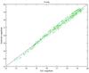 |
Fig. 1 Comparison between SExtractor and GSC2.3 magnitudes in G band. |
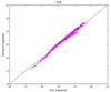 |
Fig. 2 Comparison between Sextractor and GSC2.3 magnitudes in I band. |
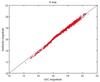 |
Fig. 3 Comparison between Sextractor and GSC2.3 magnitudes in R band. |
Figures 1−3 show the comparisons between the magnitudes computed with Sextractor and the ones of the GSC2.3 catalogue, for the objects in common. The blue line delineating the equation y = x illustrates the good agreement between these magnitudes. The systematic differences seen on the three graphs are certainly due in large part to the filters used at the CFHT not beeing exactly the same as those of the Guide Star Catalogue. They can also be due to the method used by Sextractor to compute the flux of the object (Kron’s algorithm) and also to the parameters in the default configuration file of the software (minimum number of pixels above threshold, detection threshold etc.).
3.2. Light curves of the QSOs
This paragraph is dedicated to the presentation of some light curves of the Deep 2 QSOs. As seen previously, the adjustment of the calibration constants is known with an uncertainty of roughly between 0.15 mag and 0.25 mag (1σ) depending on the filter used. It can then be considered as the uncertainty in the determination of the magnitude with SExtractor. The three curves presented here for each quasar (Figs. 4 to 14) correspond to the R (red curve), G (green curve), and I (cyan curve) bands. We clearly observe for each case a very strong correlation between the three curves indicating without ambiguity that the observed light variations are intrinsic to the quasars themselves. The time is expressed in years from the end of 2003 to mid 2007. The number at the top of a panel is the identification number of the quasar in the LQAC catalogue. The exposure time in most cases is 300 s.
Table 1 shows that among the 41 QSOs kept in our study, 26 of them (63%) have a magnitude in neither the R band nor the G and I bands. Nevertheless, these poor quality statistics do not reflect the reality of the LQAC. In the entire catalogue (113 666 sources), 14 001 sources can be found (12.3%) of which have no U band magnitude, 6865 (6.0%) no B band magnitude, 38 270 (33.7%) no V band magnitude, 38 804 (34.1%) no G band magnitude, 12 855 (11.3%) no R band magnitude, 27 428 (24.1%) no I band magnitudes. In addition 38 805 (34.1%) have no Z band magnitude. This lack of knowledge about the visual magnitudes of quasars, and their variations, must be compensated for in the future when building a robust reference system as in the radio domain for the ICRF.
4. Astrophotometry of the Deep 2 set of QSOs
We investigate the possibility that quasar photometric variability is accompanied by a displacement of the photocenter in the optical image, as it was proposed by Andrei et al. (2008). Because of the a priori very small amplitude of this displacement, a very precise astrometric measurement is necessary. To this aim, two different approaches to the astrometric treatment are proposed. The first is a classical astrometric reduction to first order of the images. The second is based on the determination and study of the PSF (point spread function) of the quasar studied. The results obtained in the two cases for the position of the quasars are compared to the light curves presented in the last section.
4.1. First method: classical astrometric reduction
Here the astrometric reduction consists of determining the positions of a quasar on a given CCD image relative to its position on a CCD image taken as a reference, called the master image. The coordinates of the center of the master image correspond to the coordinates of the D2 target field (10h0min29s and +2°12′21′′). The exposure time is 360 s in R band and the observation date is 2003 December 20. Table 3 gives the exposure number of all the images used together with the MJD of observation.
Reference of the images used to determine the position of the QSOs against the reference CCD.
4.1.1. Detection of the centroïds
The first step of the process is to obtain the centroïd x and y positions of the objects on the CCD. To achieve this, we use specialized optimized detection software, i.e. the SExtractor software, to derive the light curves in the previous section (Bertin 1996). Several methods to determine the position of the centroïd of a given target are possible with this software. We chose the Gaussian window. The pixel values are integrated within a circular Gaussian window as opposed to the object isophotal footprint. The Gaussian window is scaled to each object. Computing windowed parameters can be quite CPU intensive because of the iterative process involved. Despite this, the use of windowed parameters are recommended instead of their isophotal equivalents, as the measurements they provide are much less noisy. The positional accuracy provided by XWIN_IMAGE and YWIN_IMAGE is close to that achieved by PSF-fitting.
4.1.2. Mathematical frame
The mathematical equations that allow us to transform the x and y coordinates from a given CCD (measured with Sextractor) to the X and Y coordinates in the master CCD are given by  \arraycolsep1.75ptTo first order, these equations take into account the geometry (rotation, scale factor, and translation) between the two MEGACAM CCD chips. These equations could be expanded to higher order to take into account some optical distortions of the image or the DCR (differential chromatic refraction). Nevertheless, in this work, the simplified model above was used because of the relatively small field of a MEGACAM chip (15′ × 7′). A cross-identification of the flux selected objects found by Sextractor on the two CCDs was performed using a home-made software. The corresponding couples (x,y) and (X,Y) were then injected into the above equations and a least squares method gives the expected values of the constants A − F.
This method is differential: it has the advantage of not using any reference catalogue. The only error source should thereforebe that caused by the optical system of the telescope and atmospheric unstability during the observation.
4.1.3. Astrometric results of QSO’s centroid determinations
In this paragraph, we limit our the study to five QSOs. Their LQAC identification numbers are 39436, 39439, 39390, 39413, and 39388, and were chosen because they all come from the same CCD image. They are relatively close to each other and the corresponding CCD is not very far from the MEGACAM center. Figure 15 shows the 15th CCD where the QSOs are located.
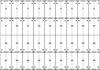 |
Fig. 15 MegaCam readout layout. North is at the top, east to the left. |
The blue curves in Figs. 16 to 18 shows the X (left column) and Y (right column) variations in time (expressed in MJD) for the five afore mentioned QSO’s compared with their magnitude (red curve). As said previously, all the positions (in pixels) have been converted to the frame of the master CCD (729989). Table 4 gives the position of the QSOs in X and Y in pixels together with its root mean square.
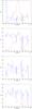 |
Fig. 16 X(t) and Y(t) positions of the QSOs 39436 and 39390 (from top to bottom) in the frame of the master CCD compared to their magnitude. The unit of measurement for the ordinate axis is arbitrary (percentage of variation) for the clarity of the graph. |
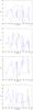 |
Fig. 17 X(t) and Y(t) positions of the QSOs 39388 and 39439 (from top to bottom) in the frame of the master CCD compared to their magnitude. The unit of measurement for the ordinate axis is arbitrary (percentage of variation) for the clarity of the graph. |
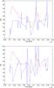 |
Fig. 18 X(t) and Y(t) positions of the QSO 39413 in the frame of the master CCD compared to his magnitude. The unit of measurement for the ordinate axis is arbitrary (percentage of variation) for the clarity of the graph. |
Mean positions and root mean square (in pixels) of the studied QSOs.
We note that all the postions are within between 0.04 px and 0.1 px around the mean position in X or Y. The 0.04 px rms is the typical best result that can be obtained with Sextractor when using the TCFH-MEGACAM images, for a pairwise comparison at high Galactic latitude, in R band and high airmass (Bertin 2007). The limit of 0.04 px corresponds to 7mas in the case of MEGACAM. Figures 16 to 18 do not provide strong evidence of a correlation between the astrometric variation in X or Y against the magnitude variation of the QSOs in the red filter. The (X,Y) measurements are in the range ±3σ, so they are dominated by the measurement noise except in some rare cases. For the QSO 39436, a correlation can be seen between the magnitude and the Y coordinate near the MJD 54 150 (February−March 2007). A large variation in the X coordinate can also be observed near the MJD 53 050 (February 2004) but cannot be correlated with a magnitude variation because of the lack of observation in the red filter. The QSO 39390 also shows a correlation between the Y coordinate and the red filter magnitude near the MJD 54 600 (April−May 2008).
To improve on these results, an independent method is used in the next paragraph.
4.2. Second method: study of the point spread function
This part of the work is based on the study of the PSF of the sources. It will be limited to the QSO 39436, which shows the greatest evidence of a correlation between its position and the variation in its R magnitude. In addition, this quasar is very close to a star (Fig. 19). That fortuitous conjunction will allow an efficient differential determination of the PSFs to substract the effect of the atmosphere. Without this comparison, it is objectively difficult to make the difference between an intrinsic variation in the QSO’s structure and a variation in its PSF caused by the atmosphere.
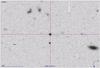 |
Fig. 19 CFHT image of the QSO 39436 with the nearby star (5′′ south). |
The distance in the sky between the star and the QSO is roughly 5′′. We can postulate that for such a very short distance, the effect of the atmosphere is the same for the QSO and the star. The difference between the QSO and the stellar profiles, if one exists, should then only be due to intrinsic variations in the structure of the QSO.
4.2.1. Mathematical frame
The point spread function describes the two dimensional distribution of light coming from a point source at the telescope focal plane. The ideal PSF is the Airy function but it is modified by the existence of the atmosphere and by the defects of the telescope’s optics (Fig. 20). A great number of PSF models are proposed in astronomy. The most popular are the Gaussian model, the Lorentzian model and the Moffat models (Moffat 1969).
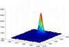 |
Fig. 20 Gaussian shape of the QSO 39436. |
In this section, we use the Gaussian model because of the simplicity of its implementation and the robustness of the results it provides.
Before processing the image, the first step is to take into account the value of the image background. A preliminary external determination must be performed in a region very near the QSO. This determination is simply the mean of the individual pixel fluxes in the region considered. This region is chosen so that it contains no bad pixel or column, no cosmic ray hits or other defects that could bias the determination of the background. It has been always possible to choose such a region. Once the background determination is performed the numerical value is subtracted from all the pixel fluxes and the Gaussian shape is determined.
The two-dimensional elliptical Gaussian function used is expressed as ![\begin{eqnarray} f(x,y)&=&A.\exp-[a\left( x-x_{0}\right) ^{2}+2b\left( x-x_{0}\right) \left( y-y_{0}\right) \nonumber \\ && + \, ... + c\left( y-y_{0}\right) ^{2}]. \end{eqnarray}](/articles/aa/full_html/2011/02/aa15500-10/aa15500-10-eq65.png) (4)In this expression, x0 and y0 are the coordinates of the blob center and A the amplitude, f(x,y) is the background substracted flux of a pixel of position (x,y) and the quantities a − c are given by
(4)In this expression, x0 and y0 are the coordinates of the blob center and A the amplitude, f(x,y) is the background substracted flux of a pixel of position (x,y) and the quantities a − c are given by 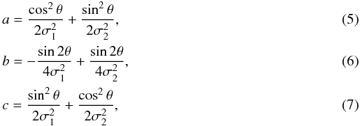 \arraycolsep1.75ptwere σ1, σ2, and θ are, respectively, the spreads and the angle of rotation (with respect to the x axis) of the blob largest axis.
The three quantities a−c can be obtained from the means of the least squares method. For this purpose, it is necessary to compute the logarithm of the expression in Eq. (4) in order to minimize the quantity ![\begin{eqnarray} \chi^{2} = \sum_{i=1}^{n}\left[ Z_{i}-\left( \alpha+\beta x_{i}+\gamma y_{i}-\left( ax_{i}^{2}+2bx_{i}y_{i}+cy_{i}^{2}\right) \right) \right] ^{2} \end{eqnarray}](/articles/aa/full_html/2011/02/aa15500-10/aa15500-10-eq76.png) (8)where Zi is the logarithm of the background-substracted flux of the pixel (xi,yi) and
(8)where Zi is the logarithm of the background-substracted flux of the pixel (xi,yi) and  \arraycolsep1.75ptEquations (9)−(11) can easily be inverted to give x0, y0, and A. In the same way, Eqs. (5)−(7) can also be inverted to give σ1, σ2, and θ.
The method described above has been implemented in customized software that yields all the Gaussian parameters (σ1, σ2, θ, A, x0, y0), which is not the case for usual detection softwares such as SExtractor or IRAF. The coordinates of the center of the Gaussian blob adjusted to the QSO’s PSF have been compared to those obtained with Sextractor. In this case, the dispersion in the coordinate difference, in both x and y, is 0.09 pixel (1σ). Other comparisons based on simulations of images (no noise added) show very good agreement between the position angles θ. This parameter is determined, in all cases, with an uncertainty much lower than 0.1° for a flattening parameter |σ1 − σ2| /σ1 larger than 10-4.
4.2.2. Results and discussion
The method presented above allows us to compare the PSFs of the star and the QSO by computing the difference between the position angles, namely |θRef.star − θQSO| with respect to the x axis. As said previously, the atmosphere or the defects in the telescope motions and optical system induce distortions in the QSO’s PSF that cannot be distinguished from intrinsic variations without the use of a relative reference, which is taken to be a nearby star in fortuitous conjunction with the QSO, 5′′ south from it. The effect of the atmosphere is then the same for the two objects and any difference between their PSFs can be interpreted as residual intrinsic variation in the QSO’s structure. Here only the position angles θ were compared. The difference between the amplitudes of the Gaussian shapes are more difficult to interpret because the two objects do not have exactly the same magnitude. The dispersions in the blobs (σ1,σ2) are of valuable interest because they give indications of the flattening of the Gaussians but are obviously related to the position angles. In all cases, the flattening of the Gaussian shapes (QSO and reference star) is between 1% and 10%/15% (marginally up to 20%).
Figure 21 shows both a red curve of photometric nature and a blue curve of astrometric one. The red one stands for the red magnitude of the QSO 39436. The blue one is the representation of the difference in position angles θ between the QSO and the star PSFs (in absolute value). The position angles were computed by our customized software based on the method explained in the last section using the observations with the red filter. For clarity, the ordinate axis is in arbitrary units so that the maximum of the curves has the value 100 and the minimum the value 0.
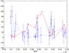 |
Fig. 21 Comparison of red magnitude with the relative position angle of the QSO 39436. |
The first period of observation goes from MJD 52 993 to MJD 53 330. During that period a large variation in the X coordinate was observed as shown in Fig. 16, which can also be discerned in the blue curve of Fig. 21. Although the θ curve seems to show a similar behaviour, the lack of red (or green) magnitude data during nearly 6 months (MJD 53 136 to MJD 53 330) for the period of interest prevents from firmly concluding in favour of a correlation. The second period of observation ranges from MJD 53 330 and MJD 53 678. During that period, the shapes of the two curves are very similar even if they are not exactly time-correlated.
The fact that the two curves be exactly time-correlated is not mandatory because the magnitude variation may be due to physical phenomenon affected by a circular symmetry. In that case, no θ variation should be detected and any correlation between the curves would be seen. No observation was performed between MJD 53 503 and MJD 53 678. The third period of observation ranges from MJD 53 678 to MJD 54 089. During that period, the shape of the two curves are once again very similar. No observation was made between MJD 53 854 and MJD 54 089. The fourth period of observation was from MJD 54 089 and MJD 54 475. Once again, the shape of the two curves are very similar but no observation was made between MJD 54 237 and MJD 54 475.
The coincidence between the magnitude and the position angle could be fortuitous. The small number of observations and that magnitude and position angle are not exactly time-correlated makes it difficult to decide in favour of real or fortuitous coincidence. Some other tests, involving several other QSO-reference star pairs, must be undertaken to give statistical arguments to discriminate between the two possibilities.
If this correlation existed for some QSO, it could allow us to easily identify among them those that were less suitable for establishing a stable extragalactic reference frame. This is an important aim for the Gaia mission and in determining the link between the radio and optical reference frames.
4.2.3. Proper motion of the reference star
As a by-product of the study presented here it is possible to determine the differential coordinates of the reference star. It will be assumed in that section that the QSO is a fixed reference point in the sky with respect to the proper motion of the star.
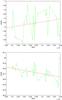 |
Fig. 22 Proper motion of the star with respect to the QSO 39436 in RA (up) and Dec (down). |
Figure 22 compares the coordinates of the two targets. The proper motion in RA is (+3.0 ±3.6) mas/y and (−6.8 ± 2.9) mas/y in Dec (the pixel scale of MEGACAM is 185 mas/pixel).
5. Conclusion and prospects
In a first part of this paper, we have presented light curves of a set of QSOs located in the Deep 2 field of the CFHT Legacy Survey in three bands corresponding to the R, G, and I filters. The time span of these time series is 4.5 years. They are characterized by magnitude variations for the three bands reaching 0.8 mag or more for a good proportion (30%) of objects. We have demonstrated that some correlations exist between the three curves (one per color) for the vast majority of the quasars. This study brings new information about the link between G, R, and I magnitudes variations, together with the finding that the QSOs in our sample are generally variable objects.
In a second part of this paper, the astrophotometric evolution of the QSOs were presented from two different points of view. A classical astrometric reduction does not exhibit strong evidence of a correlation between the magnitude variation of the QSOs and their astrometric position. Nevertheless in some particular cases, correlations can be found, particularly in the case of the QSO 39436 in the LQAC. A more precise study of the PSF distortion with the magnitude variation brings some support to the hypothesis that a variation in the position of the QSOs is linked to their optical magnitude variations. We note that the time series related to CFHT-LS observations are not precisely dedicated to astrophotometric research. Moreover, the instrument itself is not an astrometric telescope. For example, the lack of observational data prevents us from concluding firmly in favour of a correlation between the two phenomena (position and magnitude variations). Our mathematical analysis could also be improved to obtain optimal results. Despite the lack of observations, the results reported here can be seen as encouraging ones.
As a by-product of that study the proper motion of the nearby star J095940.04+022313.3 (recommended SDSS name, based on J2000 position) has been determined.
The results presented here are presently being extended to the Deep 3 and 4 fields of the CFHT-LS. For the most interesting QSOs (in term of astrophotometric variability), investigations of their PSFs with high angular resolution telescopes (VLT, HST) could be undertaken. Specific radio-optical concomitant observations are also in progress together with the VLBI team of SYRTE-OP.
At radio wavelengths the structure index (Fey 1997b) gives an indication of the astrometric quality of a source. At optical wavelengths a compacity criteria could be defined to quantify the astrometric quality of a source. We are currently attempting to define such a criterion and compile an optical QSO database in preparation for the Gaia mission.
Bourda et al. (2008) give a list of 70 sources that have excellent or good astrometric suitability (i.e. an X-band structure index value of either 1 or 2) to ensure the link between the ICRF2 and the Gaia reference frame with the highest accuracy. Optical observations of these sources are currently in progress with the 1.2 m telescope of the Haute Provence Observatory (IAU code 511) to determine if they are point sources and exhibit rapid magnitude variations (some days). If the astrophotometric
relationship were assumed, QSOs with such variations could display a scattering in their centroid of several hundred of μas, which would make these quasars less suitable for constructing a stable extragalactic reference frame. The photometric time series of quasars are also important in the framework of the Gaia working group “Initial QSO Catalogue” lead by A. Andrei.
The team of SYRTE-OP has been involved in high precision astrometry with ground-based optical telescopes since the begining of 2007. This paper present the first results we have obtained about astrophotometric variations of QSOs. We propose that this original study represents a significant contribution to establishingthe link between the reference frames ahead of the Gaia mission.
Online material
 |
Fig. 4 Comparison between G mag, R mag, and I mag for QSOs 39976, 39952, 39906 and 39764. |
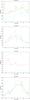 |
Fig. 5 Comparison between G mag, R mag, and I mag for QSOs 39735, 39673, 39576 and 39574. |
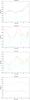 |
Fig. 6 Comparison between G mag, R mag, and I mag for QSOs 39525, 39529, 39441 and 39363. |
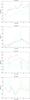 |
Fig. 7 Comparison between G mag, R mag, and I mag for QSOs 39246, 39924, 39851 and 39903. |
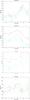 |
Fig. 8 Comparison between G mag, R mag, and I mag for QSOs 39862, 39744, 39675 and 39436. |
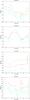 |
Fig. 9 Comparison between G mag, R mag, and I mag for QSOs 39390, 39388, 39439 and 39413. |
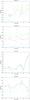 |
Fig. 10 Comparison between G mag, R mag, and I mag for QSOs 39301, 39298, 39871 and 39762. |
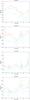 |
Fig. 11 Comparison between G mag, R mag, and I mag for QSOs 39801, 39739, 39656 and 39613. |
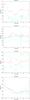 |
Fig. 12 Comparison between G mag, R mag, and I mag for QSOs 39571, 39620, 39354 and 39982. |
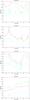 |
Fig. 13 Comparison between G mag, R mag, and I mag for QSOs 39688, 39691, 39595 and 39571. |
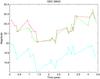 |
Fig. 14 Comparison between G mag, R mag, and I mag for QSO 39603. |
Acknowledgments
We would like to thank the referee, F. Van Leeuwen, for his useful suggestions and comments. A.H.A. acnowledges CNPq Bolsa de Pesquisa 307126 2006-4 and Marie Curie Grant PIIF GA 2009 236735 Based on observations obtained with MegaPrime/MegaCam, a joint project of CFHT and CEA/DAPNIA, at the Canada-France-Hawaii Telescope (CFHT) which is operated by the National Research Council (NRC) of Canada, the Institut National des Science de l’Univers of the Centre National de la Recherche Scientifique (CNRS) of France, and the University of Hawaii. This work is based in part on data products produced at TERAPIX and the Canadian Astronomy Data Centre as part of the Canada-France-Hawaii Telescope Legacy Survey, a collaborative project of NRC and CNRS.
References
- Andrei, A., Bouquillon, S., de Camargo, J. I. B., et al. 2008, JSRS and X. Lohrmann Kolloquium Proc., ed. M. Soffel, & N. Capitaine, 199 [Google Scholar]
- Andrei, A., Souchay, J., Zacharias, N., et al. 2009, A&A, 505, 385 [NASA ADS] [CrossRef] [EDP Sciences] [MathSciNet] [Google Scholar]
- Bertin, E. 2007, Personnal communication [Google Scholar]
- Bertin, E., & Arnouts, S. 1996, A&AS, 117, 393 [NASA ADS] [CrossRef] [EDP Sciences] [Google Scholar]
- Bourda, G., Charlot, P., & Le Campion, J. F. 2008, A&A, 490, 403 [NASA ADS] [CrossRef] [EDP Sciences] [Google Scholar]
- Feissel-Vernier, M. 2003, A&A, 403, 105 [NASA ADS] [CrossRef] [EDP Sciences] [Google Scholar]
- Feissel-Vernier, M., Ma, C., Gontier, A.-M., & Barache, C. 2006, A&A, 452, 1107 [NASA ADS] [CrossRef] [EDP Sciences] [Google Scholar]
- Fey, A. L., & Charlot, P. 1997, ApJS, 111, 95 [NASA ADS] [CrossRef] [Google Scholar]
- Fey, A. L., Eubanks, T. M., & Kingham, K. A. 1997, AJ, 114, 2284 [NASA ADS] [CrossRef] [Google Scholar]
- Fey, A. L., Ma, C., Arias, E. F., et al. 2004, AJ, 127, 3587 [NASA ADS] [CrossRef] [Google Scholar]
- Fey, A. L., Gordon, D. G., & Jacobs, C. S. 2009, IERS Technical Note, 35 [Google Scholar]
- Gontier, A.-M., Le Bail, K., Feissel, M., & Eubanks, T. M. 2001, A&A, 375, 661 [Google Scholar]
- Gupta, A. C., & Joshi, U. C. 2005, A&A, 440, 855 [NASA ADS] [CrossRef] [EDP Sciences] [Google Scholar]
- Hawkins, M. R. S. 2002, MNRAS, 329, 76 [NASA ADS] [CrossRef] [Google Scholar]
- IERS 1999, International Earth Rotation Service Annual Report 1998, Observatoire de Paris, 87 [Google Scholar]
- Kovalevsky, J., Lindegren, L., Perryman, M. A. C., et al. 1997, A&A, 323, 620 [NASA ADS] [Google Scholar]
- Kron, R. G. 1980, ApJS, 43, 305 [NASA ADS] [CrossRef] [Google Scholar]
- Lambert, S. B., & Gontier, A.-M. 2009, A&A, 493, 317 [NASA ADS] [CrossRef] [EDP Sciences] [Google Scholar]
- Lambert, S. B., Dehant, V., & Gontier, A.-M. 2008, A&A, 481, 535 [NASA ADS] [CrossRef] [EDP Sciences] [Google Scholar]
- Lasker, B. M., Lattanzi, M. G., McLean, B. J., et al. 2008, AJ, 136, 735 [NASA ADS] [CrossRef] [PubMed] [Google Scholar]
- Lindegren, L. 2009, Proc. IAU Symp., 261, 296 [Google Scholar]
- Ma, C., Arias, E. F., Eubanks, T. M., et al. 1998, AJ, 116, 516 [NASA ADS] [CrossRef] [Google Scholar]
- Moffat, A. F. J. 1969, A&A, 3, 455 [NASA ADS] [Google Scholar]
- Rabette, M., McBreen, B., Smithi, N., & Steel, S. 1998, A&AS, 129, 445 [Google Scholar]
- Smith, A. G., Nair, A. D., Leacock, R. J., et al. 1993, AJ, 105, 437 [NASA ADS] [CrossRef] [Google Scholar]
- Souchay, J., Andrei, A., Barache, C., et al. 2009, A&A, 494, 799 [NASA ADS] [CrossRef] [EDP Sciences] [Google Scholar]
- Véron-Cetty, M.-P., & Véron, P. 2006, A&A, 455, 773 [NASA ADS] [CrossRef] [EDP Sciences] [Google Scholar]
- Zacharias, N., Urban, S. E., Zacharias, M. I., et al. 2004, AJ, 127, 3043 [NASA ADS] [CrossRef] [Google Scholar]
- Zackrisson, E., Bergvall, N., Marquart, T., & Helbig, P. 2003, A&A, 408, 17 [NASA ADS] [CrossRef] [EDP Sciences] [Google Scholar]
All Tables
Example of calibration constant and root mean square in R band for some MegaCam images.
Reference of the images used to determine the position of the QSOs against the reference CCD.
All Figures
|
Fig. 1 Comparison between SExtractor and GSC2.3 magnitudes in G band. |
| In the text | |
|
Fig. 2 Comparison between Sextractor and GSC2.3 magnitudes in I band. |
| In the text | |
|
Fig. 3 Comparison between Sextractor and GSC2.3 magnitudes in R band. |
| In the text | |
|
Fig. 15 MegaCam readout layout. North is at the top, east to the left. |
| In the text | |
|
Fig. 16 X(t) and Y(t) positions of the QSOs 39436 and 39390 (from top to bottom) in the frame of the master CCD compared to their magnitude. The unit of measurement for the ordinate axis is arbitrary (percentage of variation) for the clarity of the graph. |
| In the text | |
|
Fig. 17 X(t) and Y(t) positions of the QSOs 39388 and 39439 (from top to bottom) in the frame of the master CCD compared to their magnitude. The unit of measurement for the ordinate axis is arbitrary (percentage of variation) for the clarity of the graph. |
| In the text | |
|
Fig. 18 X(t) and Y(t) positions of the QSO 39413 in the frame of the master CCD compared to his magnitude. The unit of measurement for the ordinate axis is arbitrary (percentage of variation) for the clarity of the graph. |
| In the text | |
|
Fig. 19 CFHT image of the QSO 39436 with the nearby star (5′′ south). |
| In the text | |
|
Fig. 20 Gaussian shape of the QSO 39436. |
| In the text | |
|
Fig. 21 Comparison of red magnitude with the relative position angle of the QSO 39436. |
| In the text | |
|
Fig. 22 Proper motion of the star with respect to the QSO 39436 in RA (up) and Dec (down). |
| In the text | |
|
Fig. 4 Comparison between G mag, R mag, and I mag for QSOs 39976, 39952, 39906 and 39764. |
| In the text | |
|
Fig. 5 Comparison between G mag, R mag, and I mag for QSOs 39735, 39673, 39576 and 39574. |
| In the text | |
|
Fig. 6 Comparison between G mag, R mag, and I mag for QSOs 39525, 39529, 39441 and 39363. |
| In the text | |
|
Fig. 7 Comparison between G mag, R mag, and I mag for QSOs 39246, 39924, 39851 and 39903. |
| In the text | |
|
Fig. 8 Comparison between G mag, R mag, and I mag for QSOs 39862, 39744, 39675 and 39436. |
| In the text | |
|
Fig. 9 Comparison between G mag, R mag, and I mag for QSOs 39390, 39388, 39439 and 39413. |
| In the text | |
|
Fig. 10 Comparison between G mag, R mag, and I mag for QSOs 39301, 39298, 39871 and 39762. |
| In the text | |
|
Fig. 11 Comparison between G mag, R mag, and I mag for QSOs 39801, 39739, 39656 and 39613. |
| In the text | |
|
Fig. 12 Comparison between G mag, R mag, and I mag for QSOs 39571, 39620, 39354 and 39982. |
| In the text | |
|
Fig. 13 Comparison between G mag, R mag, and I mag for QSOs 39688, 39691, 39595 and 39571. |
| In the text | |
|
Fig. 14 Comparison between G mag, R mag, and I mag for QSO 39603. |
| In the text | |
Current usage metrics show cumulative count of Article Views (full-text article views including HTML views, PDF and ePub downloads, according to the available data) and Abstracts Views on Vision4Press platform.
Data correspond to usage on the plateform after 2015. The current usage metrics is available 48-96 hours after online publication and is updated daily on week days.
Initial download of the metrics may take a while.