| Issue |
A&A
Volume 526, February 2011
|
|
|---|---|---|
| Article Number | A70 | |
| Number of page(s) | 12 | |
| Section | The Sun | |
| DOI | https://doi.org/10.1051/0004-6361/201015453 | |
| Published online | 23 December 2010 | |
A comparison of preprocessing methods for solar force-free magnetic field extrapolation
1
Institut für Physik und Astronomie, Universität Potsdam,
Karl-Liebknecht-Str. 24/25,
14476
Potsdam,
Germany
e-mail: This email address is being protected from spambots. You need JavaScript enabled to view it.
, This email address is being protected from spambots. You need JavaScript enabled to view it.
2
LESIA, Observatoire de Paris, CNRS, UPCM, Université Paris
Diderot, 5 place de Jules
Janssen, 92190
Meudon,
France
e-mail: This email address is being protected from spambots. You need JavaScript enabled to view it.
3
Max-Planck-Institut für Sonnensystemforschung,
Max-Planck-Str. 2,
37191
Katlenburg-Lindau,
Germany
e-mail: This email address is being protected from spambots. You need JavaScript enabled to view it.
Received:
22
July
2010
Accepted:
12
October
2010
Abstract
Context. Extrapolations of solar photospheric vector magnetograms into three-dimensional magnetic fields in the chromosphere and corona are usually done under the assumption that the fields are force-free. This condition is violated in the photosphere itself and a thin layer in the lower atmosphere above. The field calculations can be improved by preprocessing the photospheric magnetograms. The intention here is to remove a non-force-free component from the data.
Aims. We compare two preprocessing methods presently in use, namely the methods of Wiegelmann et al. (2006, Sol. Phys., 233, 215) and Fuhrmann et al. (2007, A&A, 476, 349).
Methods. The two preprocessing methods were applied to a vector magnetogram of the recently observed active region NOAA AR 10 953. We examine the changes in the magnetogram effected by the two preprocessing algorithms. Furthermore, the original magnetogram and the two preprocessed magnetograms were each used as input data for nonlinear force-free field extrapolations by means of two different methods, and we analyze the resulting fields.
Results. Both preprocessing methods managed to significantly decrease the magnetic forces and magnetic torques that act through the magnetogram area and that can cause incompatibilities with the assumption of force-freeness in the solution domain. The force and torque decrease is stronger for the Fuhrmann et al. method. Both methods also reduced the amount of small-scale irregularities in the observed photospheric field, which can sharply worsen the quality of the solutions. For the chosen parameter set, the Wiegelmann et al. method led to greater changes in strong-field areas, leaving weak-field areas mostly unchanged, and thus providing an approximation of the magnetic field vector in the chromosphere, while the Fuhrmann et al. method weakly changed the whole magnetogram, thereby better preserving patterns present in the original magnetogram. Both preprocessing methods raised the magnetic energy content of the extrapolated fields to values above the minimum energy, corresponding to the potential field. Also, the fields calculated from the preprocessed magnetograms fulfill the solenoidal condition better than those calculated without preprocessing.
Key words: Sun: magnetic topology / Sun: atmosphere / magnetohydrodynamics (MHD)
© ESO, 2010
1. Introduction
In order to model and understand the physical mechanisms underlying the various activity phenomena that can be observed in the solar atmosphere, like, for instance, spots, faculae, flares, and coronal mass ejections, as well as their mutual connections an interactions, the magnetic field vector throughout the atmosphere must be known. Unfortunately, reliable magnetic field measurements are still restricted to the level of the photosphere, where the inverse Zeeman effect in Fraunhofer lines is observable. Progress is very slow here, due to fundamental difficulties in unambiguously deriving the magnetic field from polarimetric measurements in chromospheric or coronal spectral lines. Other information sources, like non-burst radio emission or contrast pictures in selected spectral lines or continuum parts of the solar spectrum, provide only order-of-magnitude estimates or limited qualitative information.
As an alternative to measurements in the chromosphere and in the corona, the measured
photospheric field may be extrapolated theoretically into these higher layers of the
atmosphere. Such extrapolations are usually done under the assumption that the magnetic
field B is approximately force-free, i.e. characterized by the
equations  where
α(r) denotes a scalar function of position
r which, because of Eq. (2), is constant along the magnetic field lines. As an implication of the
dominance of the magnetic energy density over all other energy densities (cf. Gary 2001), this approximation is, except for the times
of explosive events, presumably valid from the upper chromosphere up to coronal heights of
~1 R⊙ above the photosphere.
where
α(r) denotes a scalar function of position
r which, because of Eq. (2), is constant along the magnetic field lines. As an implication of the
dominance of the magnetic energy density over all other energy densities (cf. Gary 2001), this approximation is, except for the times
of explosive events, presumably valid from the upper chromosphere up to coronal heights of
~1 R⊙ above the photosphere.
The development of extrapolation methods began with calculations of potential fields, which correspond to the case of α = 0, either above limited photospheric areas, in particular active regions (Schmidt 1964; Teuber et al. 1977), or in spherical shells above the full photosphere (Schatten et al. 1969; Altschuler & Newkirk 1969). Extrapolation methods using linear force-free fields, which correspond to the case of a spatially constant non-vanishing α, followed as a next step. Corresponding solutions were given by Nakagawa & Raadu (1972), Chiu & Hilton (1977), Seehafer (1978), Alissandrakis (1981), Semel (1988); see also reviews and comparisons by Seehafer (1982), Seehafer & Staude (1983), Gary (1989), and Sakurai (1989).
Over the last three decades, extrapolation methods for nonlinear force-free fields were also developed. Here α is allowed to vary spatially. Unlike the extrapolation methods for current-free and constant-α force-free fields, which require only line-of-sight magnetograms, the non-constant-α force-free fields are calculated from photospheric vector magnetograms. Presently great efforts are made to improve the methods used here. They include (i) direct vertical integration schemes (Wu et al. 1985, 1990; Cuperman et al. 1990; Démoulin et al. 1992; Song et al. 2006); (ii) Grad-Rubin methods (Grad & Rubin 1958; Sakurai 1981; Aly & Seehafer 1993; Amari et al. 1997, 1999, 2006; Wheatland 2004, 2006); (iii) boundary-integral methods (Yan & Sakurai 1997, 2000; Yan 2003; Yan & Li 2006; He & Wang 2006); (iv) relaxation methods (Yang et al. 1986; Mikic & McClymont 1994; Roumeliotis 1996; Valori et al. 2005); and (v) optimization methods (Wheatland et al. 2000; Wiegelmann 2004, 2007). Discussions and quantitative tests and comparisons of the nonlinear extrapolation methods are found, e.g., in Aly (1989), Sakurai (1989), McClymont et al. (1997), Schrijver et al. (2006), Metcalf et al. (2008), Schrijver et al. (2008), Wiegelmann (2008), and DeRosa et al. (2009).
Applied to semi-analytical force-free test fields (Low & Lou 1990; Titov & Démoulin 1999), the nonlinear extrapolation methods show encouraging results (Schrijver et al. 2006; Wiegelmann et al. 2006a; Valori et al. 2007, 2010). Nevertheless, most of these methods are still lacking a sound mathematical basis. The existence of solutions seems to have been proven merely for Grad-Rubin methods, and here only for sufficiently small |α| , i.e. close to the potential field (Bineau 1972; Kaiser et al. 2000; Boulmezaoud & Amari 2000). The Grad-Rubin methods do not exploit the full information content of photospheric vector magnetograms (the normal field component Bn and α are used as boundary data, but α is prescribed only on a part of the boundary where Bn is either positive or negative).
By contrast, the fields calculated by direct vertical integration always satisfy the conditions given by the photospheric vector magnetograms, and are valid and uniquely determined solutions to the problem, whenever such solutions exist and are sufficiently smooth. The solutions are however unstable, or the problem is ill-posed, in the sense that small changes of the photospheric boundary values can lead to large changes of the field above the photosphere.
The boundary-integral, relaxation and optimization methods, on the other hand, impose conditions on all three components of the magnetic vector on the complete boundary of the solution domain, mostly a rectangular cuboid or a spherical shell above the photosphere, with some assumtion for the non-photospheric parts of the boundary. This way the instability of the solution to boundary-value perturbations is avoided, but inconsistencies in the boundary values lead to only partially force- and divergence-free reconstructions. Therefore, the prescribed boundary values cannot be arbitrary but have to satisfy consistency conditions. This consistency of the data with the condition of force-freeness cannot be expected in practice, however, because (i) the field is not force-free in the photosphere and in the lower chromosphere (possibly with the exception of regions with particularly strong fields, like sunspots); and (ii) compatibility with the condition of force-freeness, if it were given for a real photospheric field, would be destroyed by measurement errors, which are always present, in particular in the transverse field components (perpendicular to the line of sight of the observer), e.g. caused by systematic uncertainties (typically much larger for the transverse than for the longitudinal field components), or by an inappropriate resolution of the 180° ambiguity.
The compatibility of the boundary data with the condition of force-freeness can be improved by an appropriate preprocessing of the data. Algorithms for such a preprocessing have been suggested by Wiegelmann et al. (2006b) and Fuhrmann et al. (2007). Their strategy is to modify the magnetographic data within certain margins such as to minimize the total magnetic force and the total magnetic torque on the volume considered. These integral quantities vanish if the magnetic field is force-free, and can be expressed as a function of the boundary values of B alone (Molodenskii 1969; Aly 1984, 1989; Low 1985). The minimization process removes a non-force-free component from the data, so that the resulting boundary values can be more consistently extrapolated into a force-free field.
Another, related objective of the preprocessing is to remove small-scale noise from the data. It has been observed that the convergence of the evolutionary or iterative sequences calculated using the relaxation or optimization methods can worsen sharply due such a noise, and the quality of the obtained solutions, that is, the degree to which they are force-free, is also worsened. This phenomenon is not well understood presently.
One aim of smoothing the photospheric magnetogram is also to mimic the expansion of the solar magnetic field between photosphere and chromosphere, where the field is assumed to become force-free. The idea is that force-free models are only valid above the chromosphere, but not suitable for modelling the high-beta plasma between photosphere and chromosphere; see also discussion in Metcalf et al. (2008). In this sense the preprocessed field may be considered as an approximation to the chromospheric field, which is much smoother and shows less fine structures than the photospheric field. Jing et al. (2010) compared unprocessed and preprocessed photospheric field measurements from Hinode with chromospheric field measurements from Solis and found that the preprocessed field is indeed a reasonable approximation of the chromospheric field.
In this paper, we compare the preprocessing methods of Wiegelmann et al. (2006b), hereafter ppTW, and Fuhrmann et al. (2007), hereafter ppMF. In particular, the two methods are applied to a vector magnetogram of a recently observed active region, NOAA active region (AR) 10 953, which has been the target in a comparitative study of different extrapolation methods for nonlinear force-free magnetic fields reported in DeRosa et al. (2009).
The remainder of the paper is organized as follows: In Sect. 2 we describe the two preprocessing methods. Then, in Sect. 3, we apply them to AR 10 953: in Sect. 3.1 some observational details of AR 10 953 and of the data used are given, and in Sects. 3.2 and 3.3 the effects of the preprocessing on the magnetogram and on the extrapolated field, respectively, are analyzed. In Sect. 4, we draw conclusions and discuss our results.
2. Preprocessing algorithms
2.1. General strategy
The general strategy of ppTW and ppMF is to modify the boundary data given by the photospheric vector magnetogram in order to decrease the total force and the total torque on the volume considered and to reduce the amount of small-scale noise in the data. This is done by minimizing a functional L of the boundary values of B. L is the sum of a number of subfunctionals each of which measures one of the quantities to be made small, i.e., the total force, the total torque, and the amount of noise. The degree of deviation of the modified photospheric fields from the original one during the minimization is controlled either via an additional subfunctional of L that measures the deviation, or by allowing the modification of the data only within prescribed domain borders. The different subfunctionals of L are weighted in order to control their relative importance for the minimization.
2.1.1. Total magnetic force and total magnetic torque
Let 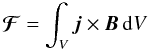 (3)denote the total
magnetic force and
(3)denote the total
magnetic force and 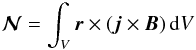 (4)the total magnetic
torque on the volume V, the solution domain. In Cartesian
coordinates x, y, z, with the
z axis pointing upward in the atmosphere, and with S
denoting the magnetogram area in the plane z = 0, the condition
ℱ = 0 is approximated by
(4)the total magnetic
torque on the volume V, the solution domain. In Cartesian
coordinates x, y, z, with the
z axis pointing upward in the atmosphere, and with S
denoting the magnetogram area in the plane z = 0, the condition
ℱ = 0 is approximated by
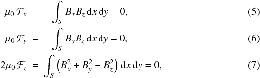 while
the condition
while
the condition  is approximately expressed by
 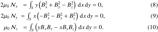 (Molodenskii 1969; Aly
1989; Fuhrmann et al. 2007). For
expressing the conditions of vanishing force and torque on V exactly,
the integrals on the right-hand sides of Eqs. (5)–(10) would have to be
extended to integrals over the complete surface ∂V of
V. The restriction to integrations over the photospheric magnetogram
area S is done under the assumption that all relevant magnetic flux
is closed on the photosphere, and the field on the rest of the boundary is so weak that
its contribution to the surface integrals for ℱ and
(Molodenskii 1969; Aly
1989; Fuhrmann et al. 2007). For
expressing the conditions of vanishing force and torque on V exactly,
the integrals on the right-hand sides of Eqs. (5)–(10) would have to be
extended to integrals over the complete surface ∂V of
V. The restriction to integrations over the photospheric magnetogram
area S is done under the assumption that all relevant magnetic flux
is closed on the photosphere, and the field on the rest of the boundary is so weak that
its contribution to the surface integrals for ℱ and
 is negligible.
2.1.2. Smoothing
There are several methods for removing small-scale irregularities from a noisy vector magnetogram, hereafter called smoothing (Press et al. 1989). We restrict ourselves to the discussion of the two smoothing methods employed by the codes discussed below.
The first method consists in applying the two-dimensional Laplacian, Δxy = ∂2/∂x2 + ∂2/∂y2, to the photospheric field, B(x,y,z = 0), and minimizing the integral of the square of the obtained function, [ΔxyB(x,y,z = 0)]2, over the magnetogram area. [ΔxyB(x,y,z = 0)]2 measures the roughness of the photospheric boundary data, and minimizing it corresponds to recducing the deviations of the field values at given points from the mean values of the field in points around them, in accordance with the mean-value property of the harmonic functions. Since the second-order derivatives measure the curvature of the surfaces Bx(x,y,z = 0), By(x,y,z = 0), and Bz(x,y,z = 0), decreasing the modulus of ΔxyB(x,y,z = 0) to zero on S would remove all global or local maxima or minima of the three field components (except for those on the boundary line of the magnetogram), including the physically significant ones, and the total energy content of the field might be strongly reduced. This kind of smoothing may however well mimic the expansion of the magnetic field between photosphere and chromosphere.
The second smoothing method considered here is the windowed-median method (Press et al. 1989). Compared to the first method, essentially the normal, arithmetic mean is replaced by the median. That is, one calculates the median of the field values in a small window around a given grid point and then minimizes the difference between the field value at the grid point and the median of the window. This way one tries to avoid a too strong influence of large disturbances that occur only in a small number of points. Also, the structures in the measured fields may be better conserved even if the quantity minimized here is decreased to zero. In general, however, decreasing the total force and the total torque on the one hand and smoothing on the other hand are competing objectives, so that a too strong smoothing would prevent a sufficient reduction of the total force and the total torque.
2.2. Preprocessing to mimic the chromospheric field (ppTW)
Wiegelmann et al. (2006b) developed a
preprocessing routine in which the ideas described above are implemented. In discretized
form, the square of the total magnetic force, as approximated by Eqs. (5)–(7), is given by 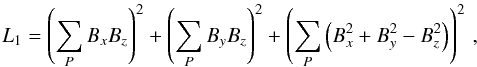 (11)and the square of the
total magnetic torque, as approximated by Eqs. (8)–(10), by
(11)and the square of the
total magnetic torque, as approximated by Eqs. (8)–(10), by 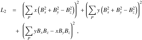 (12)where
the summation is over the points P of a photospheric grid (in the
numbering of the different subfunctionals we follow Wiegelmann et al. 2006b).
(12)where
the summation is over the points P of a photospheric grid (in the
numbering of the different subfunctionals we follow Wiegelmann et al. 2006b).
Wiegelmann et al. (2006b) used a
Laplacian-smoothing method (first method in Sect. 2.1.2) in order to reduce the amount of small-scale irregularities in the
magnetogram. The corresponding smoothing functional is calculated as ![Mathematical equation: \begin{equation} L_4^{(\mathrm{TW})} = \sum_P\left[\left(\Delta_{xy} B_x\right)^2 + \left(\Delta_{xy} B_y\right)^2 + \left(\Delta_{xy} B_z\right)^2\right] \,.\label{eq:L4TW} \end{equation}](/articles/aa/full_html/2011/02/aa15453-10/aa15453-10-eq38.png) (13)A further subfunctional
implemented in ppTW measures the difference between the preprocessed
magnetogram and the original, observed one,
(13)A further subfunctional
implemented in ppTW measures the difference between the preprocessed
magnetogram and the original, observed one, ![Mathematical equation: \begin{equation} \label{L3TW} L_3 = \sum_P \left[\left(B_x - B_x^{(\mathrm{obs})} \right)^2 + \left(B_y - B_y^{(\mathrm{obs})} \right)^2 + \left(B_z - B_z^{(\mathrm{obs})} \right)^2\right], \end{equation}](/articles/aa/full_html/2011/02/aa15453-10/aa15453-10-eq39.png) (14)where
B(obs) corresponds to the observed field
values.
(14)where
B(obs) corresponds to the observed field
values.
The complete minimization functional is then given as the sum  (15)where
 are
yet undetermined weighting factors. For minimizing this functional, ppTW
employs a fast and simple Newton-Raphson scheme (Press et al. 1989).
are
yet undetermined weighting factors. For minimizing this functional, ppTW
employs a fast and simple Newton-Raphson scheme (Press et al. 1989).
As an extension of the functional given by Eq. (15), Wiegelmann et al. (2008) implemented another “L5” term, which allows to incorporate direct chromospheric observations, e.g. Hα images, into the preprocessing scheme. This can improve the approximation of the chromospheric field, in particular the transverse components, from photospheric measurements by preprocessing. The ppTW preprocessing scheme has currently been implemented and tested in spherical geometry by Tadesse et al. (2009).
2.3. Pattern-preserving preprocessing (ppMF)
In ppMF, the total magnetic force and the total magnetic torque are
calculated in the same way as in ppTW, namely using Eqs. (11) and (12). Additionally, the two quantities are made dimensionless by
normalizing L1 to ![Mathematical equation: \begin{equation} \label{NL1} N_{L_1} = \left[ \sum_P \left(\vec{B}^{(\mathrm{obs})}\right)^2 \right]^2 \end{equation}](/articles/aa/full_html/2011/02/aa15453-10/aa15453-10-eq45.png) (16)and
normalizing L2 to
(16)and
normalizing L2 to ![Mathematical equation: \begin{eqnarray} \label{NL2} N_{L_2} &=& \left[\sum_P \sqrt{x^2+y^2} \left(\vec{B}^{(\mathrm{obs})}\right)^2 \right]^2 \nonumber \\ &=&h^2\left[\sum_{k=1}^{N_x}\sum_{l=1}^{N_y}\sqrt{k^2+l^2} \left(\vec{B}^{(\mathrm{obs})}_{kl}\right)^2 \right]^2 \, , \end{eqnarray}](/articles/aa/full_html/2011/02/aa15453-10/aa15453-10-eq47.png) (17)with
Nx and
Ny denoting the numbers of grid points in
the x and y directions
(Nx Ny = N),
h the grid spacing (assumed to be equal in the x and
y directions) and
(17)with
Nx and
Ny denoting the numbers of grid points in
the x and y directions
(Nx Ny = N),
h the grid spacing (assumed to be equal in the x and
y directions) and  the elements of the magnetogram matrix. The normalized quantities
L1/NL1
and
L2/NL2
are independent of the units of length and magnetic field and both are typically ~1 for
a field that is neither force-free nor torque-free.
the elements of the magnetogram matrix. The normalized quantities
L1/NL1
and
L2/NL2
are independent of the units of length and magnetic field and both are typically ~1 for
a field that is neither force-free nor torque-free.
For the smoothing, ppMF uses a windowed-median technique (second method
in Sect. 2.1.2). In discretized form, the smoothing
functional is given as ![Mathematical equation: \begin{eqnarray} L_4^{(\mathrm{MF})} = \sum_{i=x,y,z} \sum_P & \Big\{ M_{n}\Big[B_i(x-n \,\, h,y-n \,\, h),\dots \nonumber \\ &\dots,B_i(x+n \,\, h,y+n \,\, h)\Big] - B_i(x,y) \Big\}^2 , \label{eq:L4MF} \end{eqnarray}](/articles/aa/full_html/2011/02/aa15453-10/aa15453-10-eq56.png) (18)where
n is a positive integer number and
Mn the median of a rectangular window
with (2n + 1) (2n + 1) grid points centered about
the point (x,y). The values at the boundary of the magnetogram, where the
method cannot be applied, are left unchanged; these values are expected to be small. Also,
in the practical extrapolations an artificial margin where the field vanishes is in
general added to the magnetogram.
(18)where
n is a positive integer number and
Mn the median of a rectangular window
with (2n + 1) (2n + 1) grid points centered about
the point (x,y). The values at the boundary of the magnetogram, where the
method cannot be applied, are left unchanged; these values are expected to be small. Also,
in the practical extrapolations an artificial margin where the field vanishes is in
general added to the magnetogram.
 is
normalized to
is
normalized to ![Mathematical equation: \begin{eqnarray} \label{NL4} N_{L_4^{(\mathrm{MF})}} &=& \sum_{i=x,y,z} \sum_P \Big\{ M_{n}\Big[B_i^{(\mathrm{obs})}(x-n h,y-n h),\dots\nonumber \\ &\quad \dots &, B_i^{(\mathrm{obs})}(x+n h,y+n h)\Big] + B_i^{(\mathrm{obs})}(x,y) \Big\}^2, \end{eqnarray}](/articles/aa/full_html/2011/02/aa15453-10/aa15453-10-eq62.png) (19)so
that the normalized quantity
(19)so
that the normalized quantity  is ~1 for a field of maximum roughness.
The total functional minimized in ppMF is then 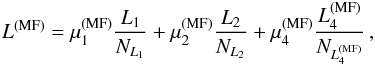 (20)with weighting factors
 ,
,
 , and
, and
 , and
for the minimization the method of simulated annealing is used (see, e.g., Press et al. 1989).
, and
for the minimization the method of simulated annealing is used (see, e.g., Press et al. 1989).
Most important, differently from ppTW, ppMF does not use the subfunctional L3, which provides a global measure of the difference between the modified and original photospheric fields. Instead, domain borders that must not be overstepped are prescribed locally at each grid point of the vector magnetogram, different for the line-of-sight and transverse field components. In this way, modifications induced by the ppMF algorithm into the measured field can be consistently limited to an estimation of the measurement errors. In the present study (Sect. 3 below) we work with overall domain borders of 120 G for the normal field and 250 G for the transverse field, but the method may be refined by applying domain borders that vary from point to point.
3. Application of the two preprocessing routines to AR 10 953
In this section, the two preprocessing routines described in Sect. 2, ppTW and ppMF, are applied to a vector magnetogram of AR 10 953, and the changes in the magnetogram due to the preprocessing are examined. After that, the preprocessed magnetograms, as well as the original one, are each extrapolated with two different methods, namely the magnetofrictional relaxation method of Valori et al. (2007) and the optimization method of Wiegelmann (2004), and the resulting fields are analyzed.
AR 10 953 has recently been studied using vector magnetograms by Okamoto et al. (2008), Su et al. (2009), and DeRosa et al. (2009). In particular, the main aim of the study by DeRosa et al. was to judge the quality of different extrapolation methods. Here, the attention is focused on the implications of using different preprocessing methods.
3.1. NOAA AR 10 953 and data used
NOAA AR 10 953 was a moderately flare-active region with a basically bipolar magnetic structure. The vector magnetogram employed here is identical to the one used in the study of DeRosa et al. (2009). It was derived from the Stokes profiles of the two magnetically sensitive Fe I lines at 6301.5 Å and 6302.5 Å measured by the Spectro-Polarimeter (SP) instrument of the Solar Optical Telescope (SOT; Tsuneta et al. 2008) onboard the Hinode satellite (Kosugi et al. 2007). The corresponding scan of the active region began at 22:30 UT on 2007 April 30 and took about 30 min. The angular resolution in the East-West and North-South directions was 0.32′′. The 180° ambiguity in the transverse field was removed by means of the AZAM utility (Lites et al. 1995; Metcalf et al. 2006). More details on the preparation of the vector magnetogram may be found in Schrijver et al. (2008) and DeRosa et al. (2009), and references given in these papers.
The area of the Hinode/SOT-SP scan covers the central part of AR 10 953, which was dominated by a leading spot of negative polarity. The active region was flare-quiet above the C1.0 level until about two days after the scan. Images from the Hinode X-Ray Telescope (XRT; Golub et al. 2007; Kano et al. 2008) taken around the time of the scan show bright loops that probably make visible bundles of coronal magnetic field lines, see Fig. 1a.
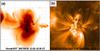 |
Fig. 1 Two coaligned images of AR 10 953 (with the same 10 degree gridlines drawn on both images for reference). a) Time-averaged and logarithmically scaled Hinode/XRT soft X-ray image; and b) STEREO-A/SECCHI-EUVI 171 Å image. |
Similar bundles of field lines are apparently seen in images from the extreme ultraviolet imagers (EUVI), which are parts of the Sun Earth Connection Coronal and Heliospheric Investigation (SECCHI) telescope packages (Howard et al. 2008) onboard the two Solar Terrestrial Relations Observatory (STEREO) spacecraft, see Fig. 1b.
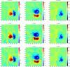 |
Fig. 2 Original and preprocessed vector magnetograms of AR 10 953. From left to right: Bx, By, and Bz. From top to bottom: Unpreprocessed, ppTW, and ppMF. The magnetic field is measured in G and the length unit is pixel (580 km). |
A significant part of the area of the vector magnetogram seems to be magnetically connected to regions outside this area. This is, for instance, also indicated by three-dimensional trajectories of loops as stereoscopically determined (Aschwanden et al. 2008) from STEREO/SECCHI-EUVI images (not shown here, see Fig. 1 in DeRosa et al. 2009).
In the study of DeRosa et al. (2009), the vector magnetogram was therefore embedded in a larger line-of-sight magnetogram with a lower spatial resolution, observed by the Michelson Doppler Imager (MDI) instrument (Scherrer et al. 1995) onboard the Solar and Heliospheric Observatory (SOHO) spacecraft. The total magnetogram used comprises, in a tangential plane to the photosphere, 320 × 320 pixel2, with 1 pixel = 580 km, so that altogether an area of 185.6 Mm × 185.6 Mm is covered, whereas the measured full magnetic vector is available for a subarea of 100 Mm × 115 Mm. The photospheric 320 × 320 pixel2 region in turn is part of an encompassing 512 × 512 pixel2 region for which a line-of-sight magnetogram was available from the SOHO/SDI measurements, and from this 512 × 512 pixel2 line-of sight magnetogram the potential field in a 512 × 512 × 512 pixel3 cube above the photosphere was calculated using a Green’s function method described in Metcalf et al. (2008) (with the normal field component set equal to zero at the side and top faces of the cube). In the study of DeRosa et al. (2009), the solution domain for the nonlinear force-free fields was then a cuboid with a height of 256 pixels above the 320 × 320 pixel2 magnetogram, with the boundary conditions at the side and top faces, for the methods that need such conditions, given by the potential field calculation for the encompassing 512 × 512 × 512 pixel3 cube, and assuming the photospheric field outside the measured vector magnetogram to be vertical, i.e., setting the horizontal field components to zero there.
Here, the preprocessing algorithms are applied to the enlarged, 320 × 320 pixel2 vector magnetogram. The subsequent analysis of the effects of the preprocessing on the photospheric field is only in part done for this enlarged magnetogram and otherwise restricted to the smaller photospheric region where the magnetic vector was measured.
3.2. Effects of the preprocessing routines on the vector magnetogram
In this subsection, the preprocessed vector magnetograms are analysed with respect to the differences they show compared to the observed magnetogram and to each other. Namely, we try to assess the smoothness of the magnetograms and how well they satisfy the conditions of force-freeness and torque-freeness. Furthermore, the function α(r) defined by Eq. (1), whose values in the level of the photosphere can be calculated from the magnetogram, is considered. This function contains much information on the topology of the magnetic field lines. In particular, the field lines lie in the surfaces α = const. and, thus, α must have equal values at any two photospheric points that are connected by a field line above the photosphere. Finally, the deviations from the original magnetogram produced by the two preprocessing methods are compared.
The minimization functionals, given by Eqs. (15) and (20), depend on the
weighting factors  and
and
 ,
respectively, which are free parameters (actually only their ratios count, so that for
each of the procedures one of the factors can be set equal to unity). The optimal choice
of the weighting factors poses a special problem of the preprocessing. As mentioned in
Sect. 2.1.2, minimizing the total magnetic force
and the total magnetic torque on the one hand and the noise level on the other hand are
competing objectives. If, for instance, the weight of smoothing in the minimization
functional is set to zero, the subfunctionals measuring the forces and torques are
generally found to be minimized very fast to very small values. If smoothing is included,
however, the reduction of the forces and torques is impeded. On the other hand, a strong
weighting of the forces and torques inhibits the smoothing (cf. consideration of this
problem in Fuhrmann et al. 2007).
,
respectively, which are free parameters (actually only their ratios count, so that for
each of the procedures one of the factors can be set equal to unity). The optimal choice
of the weighting factors poses a special problem of the preprocessing. As mentioned in
Sect. 2.1.2, minimizing the total magnetic force
and the total magnetic torque on the one hand and the noise level on the other hand are
competing objectives. If, for instance, the weight of smoothing in the minimization
functional is set to zero, the subfunctionals measuring the forces and torques are
generally found to be minimized very fast to very small values. If smoothing is included,
however, the reduction of the forces and torques is impeded. On the other hand, a strong
weighting of the forces and torques inhibits the smoothing (cf. consideration of this
problem in Fuhrmann et al. 2007).
For the results presented in the following, the weighting factors are chosen such that
the competing minimization objectives appear properly balanced. The weighting factors for
ppTW are chosen as  ,
,
 ,
,
 , and those for
ppMF as
, and those for
ppMF as  . ppTW uses
a normalization of the magnetic field to the mean value of
. ppTW uses
a normalization of the magnetic field to the mean value of
 over the magnetogram and of lengths to the edge length of the magnetogram; so the
subfunctionals of L(TW) and their weighting factors are
dimensionless but, unlike the corresponding quantities in ppMF, not
independent of the chosen units of magnetic field and length (thus the parameters cannot
be compared directly). Furthermore, ppMF is carried out with a window
size of n = 1 for the smoothing and with domain borders of 120 G for
the normal field component and of 250 G for the transverse field components during the
minimization.
over the magnetogram and of lengths to the edge length of the magnetogram; so the
subfunctionals of L(TW) and their weighting factors are
dimensionless but, unlike the corresponding quantities in ppMF, not
independent of the chosen units of magnetic field and length (thus the parameters cannot
be compared directly). Furthermore, ppMF is carried out with a window
size of n = 1 for the smoothing and with domain borders of 120 G for
the normal field component and of 250 G for the transverse field components during the
minimization.
Figure 2 shows outcomes of preprocessing the measured vector magnetogram by the two methods. Obviously, ppTW leads to a markedly smoother vector magnetogram than ppMF. Small-scale irregularities are largely removed by ppTW. The Laplacian smoothing used by this method resembles a diffusion process. Correspondingly, originally separated maxima or minima may be fused, as is seen for the By component in Fig. 3,
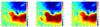 |
Fig. 3 By in a magnified cutout of the vector magnetogram of AR10 953. From left to right: Unpreprocessed, ppTW, and ppMF. The magnetic field is measured in G and the length unit is pixel (580 km). |
where a magnification of the central part of the magnetogram region is shown. By
contrast, though also smoothing the magnetogram, ppMF manages to stay
close to the observed structures. The reason for the different smoothing levels seems to
be rooted in the different smoothing schemes. The subfunctional
 ,
defined by Eq. (18), decreases very fast
during the preprocessing, without changing the magnetogram very much. Experiments for
ppMF with a Laplacian smoothing led to much smoother magnetograms, but
the decrease rate of the smoothing subfunctional,
,
defined by Eq. (18), decreases very fast
during the preprocessing, without changing the magnetogram very much. Experiments for
ppMF with a Laplacian smoothing led to much smoother magnetograms, but
the decrease rate of the smoothing subfunctional,  , was
smaller than that of the correponding subfunctional,
, when
applying the windowed-median smoothing.
, was
smaller than that of the correponding subfunctional,
, when
applying the windowed-median smoothing.
A quantitative comparison of the two preprocessing routines is given in Table 1.
The values of the total magnetic force and and the total magnetic torque shown there were calculated according to Eqs. (11) and (12) and subsequently normalized to the quantities given by Eqs. (16) and (17), respectively.
ppTW was able to decrease the total force and the total torque by two orders of magnitude. The measured total force after application of ppMF is even decreased by four orders of magnitude compared to the original total force, and the measured total torque after application of ppMF is roughly by a factor of two smaller than that after application of ppTW.
We argue that the reason for the differences in the capabilities to reduce the total magnetic force and the total magnetic torque lies in the scheme of the simulated annealing used for the minimization in ppMF, compared to the Newton-Raphson scheme employed by ppTW. While ppTW is forced to stop at the nearest local minimum it can find, ppMF is able to leave this minimum and may find another one. In Fig. 4, which shows the evolutions of the total functional L(MF) and of the sum of the normalized total force and the normalized total torque in the course of the minimization in ppMF, one can see that after roughly 1000 iterations a local minimum is found, but then this minimum is left to find a deeper one after about 2000 iterations. The values of force and torque in the first minimum are approximately the ones of ppTW. So it seems possible that ppTW was forced to stay at this minimum. An alternative possibility is that ppTW was able to find the global minimum, but that for the parameters chosen, for instance as a result of stronger smoothing, the above minimum is not the deepest one. Furthermore, the pathways of the minimization in the two algorithms will in general be different.
While for the enlarged, 320 × 320 pixel2 magnetogram, to which the
preprocessing is applied, the net flux per unit area pixel2,
 (21)nearly vanishes
(unpreprocessed: 2 × 10⁻⁷, ppTW:
3 × 10⁻⁷, ppMF: 4 × 10⁻⁷), the vector magnetogram
is not flux balanced to the same degree, see third row in Table 1. ppTW preserves the measured net flux through the
vector magnetogram area, while ppMF increases it slightly. For the
enlarged, 320 × 320 pixel2 field of view, both preprocessing routines leave the
flux balanced. So ppMF moderately redistributes the magnetic flux between
the area of the vector magnetogram and its surroundings.
(21)nearly vanishes
(unpreprocessed: 2 × 10⁻⁷, ppTW:
3 × 10⁻⁷, ppMF: 4 × 10⁻⁷), the vector magnetogram
is not flux balanced to the same degree, see third row in Table 1. ppTW preserves the measured net flux through the
vector magnetogram area, while ppMF increases it slightly. For the
enlarged, 320 × 320 pixel2 field of view, both preprocessing routines leave the
flux balanced. So ppMF moderately redistributes the magnetic flux between
the area of the vector magnetogram and its surroundings.
The fourth and fifth rows of Table 1, and
Fig. 5 show how the preprocessing routines change
the function  (22)Since this
quantity depends on all three vector components, and is sensitive to noise due to the
differentiations needed to calculate it, it is expected to be particularly strongly
affected by the preprocessing. The maximum absolute value of α is
significantly decreased by both procedures (by about 50% by ppTW and by
about 35% by ppMF, see fourth row in Table 1). The mean value of |α| over the vector
magnetogram area, on the other hand, is only weakly changed by both procedures (fifth row
in Table 1). The unpreprocessed α
function shown in Fig. 5 (left) is highly complex and
predominantly negative. ppTW yields a much smoother α
than does ppMF (Fig. 5, middle and
right), confirming the above observation that ppTW tends to remove
small-scale structures much more than ppMF.
(22)Since this
quantity depends on all three vector components, and is sensitive to noise due to the
differentiations needed to calculate it, it is expected to be particularly strongly
affected by the preprocessing. The maximum absolute value of α is
significantly decreased by both procedures (by about 50% by ppTW and by
about 35% by ppMF, see fourth row in Table 1). The mean value of |α| over the vector
magnetogram area, on the other hand, is only weakly changed by both procedures (fifth row
in Table 1). The unpreprocessed α
function shown in Fig. 5 (left) is highly complex and
predominantly negative. ppTW yields a much smoother α
than does ppMF (Fig. 5, middle and
right), confirming the above observation that ppTW tends to remove
small-scale structures much more than ppMF.
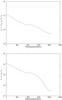 |
Fig. 4 Evolution of the total functional L(MF) as given by
Eq. (20) (top)
and of the sum |
Finally, Table 2 shows the absolute values of the differences between the preprocessed and the observed magnetograms, see also Fig. 6. ppTW leads to great changes in strong field areas, but leaves weak field areas mostly unchanged. ppMF, on the other hand, changes the whole magnetogram, but not as strongly as ppTW. The average changes of Bx, By, and Bz over the vector magnetogram are nearly identical for ppTW and ppMF. The differences between the two methods may result from the fact that in ppTW the deviation from the original magnetogram is controlled globally via the subfunctional L3, while ppMF uses a local control at each grid point.
3.3. Effects of the preprocessing on the results of extrapolations
The observed and the two preprocessed maps of the photospheric magnetic field vector are now used as input data for extrapolations using the optimization method of Wiegelmann (2004) and the magnetofrictional relaxation method of Valori et al. (2007).
The side and top boundaries are treated differently by the two extrapolation methods. The method of Wiegelmann (2004) prescribes the magnetic vector as given by an initial potential field. Our extrapolations with this method are done, as the extrapolations in DeRosa et al. (2009) were done, for a cuboid above the enlarged vector magnetogram, and with the boundary condions at the side and top boundaries given by the values of the potential field calculated for the encompassing 512 × 512 × 512 pixel3 cube. Contradictions between strong currents in the region above the vector magnetogram and the assumption of a potential magnetic field at the side boundaries can be mitigated by placing the side boundaries far away from the vector magnetogram area.
The method of Valori et al. (2007), as used here, applies a special kind of open boundary conditions at the side and top boundaries, where the normal field component is determined from inner field values such as to ensure the solenoidal property of B, and the transverse field is obtained from a fourth-order polynomial extrapolation of interior field values to the boundary; this precedure works with a buffer layer of three grid points at the boundaries. These special boundary conditions allow extrapolations without assuming a potential field at the side and top boundaries. Accordingly, our extrapolations using the method of Valori et al. (2007) start from the smaller photospheric area of the vector magnetogram. That is to say, the solution domain for these extrapolations is a cuboid with a height of 256 pixels above the measured vector magnetogram. The necessity of modelling the transverse photospheric field outside the vector magnetogram area is avoided. Such modelling normally produces unphysical current concentrations at and above the boundary of the vector magnetogram. Indeed, using the Valori et al. method with an embedding in the larger line-of-sight magnetogram (DeRosa et al. 2009) leads to worse extrapolation results.
The potential field calculated for the encompassing 512 × 512 × 512 pixel3 cube provides the intial field for both types of nonlinear force-free field computations. The analysis of the extrapolation results is always restricted to a cuboid above the area of the measured vector magnetogram, still slightly reduced by the Valori et al. buffer layer.
For measuring the degree of force-freeness of the extrapolated fields, we use the metric
(cf. Wheatland et al. 2000; Schrijver et al. 2006; Valori et al.
2007; DeRosa et al. 2009)  (23)where
the summation is over the grid points in the considered three-dimensional domain
V. This is a current-weighted average of the sine of the angle
θ between the magnetic field B and the
current density J, with
CWsin = 0 for an exactly force-free
magnetic field.
(23)where
the summation is over the grid points in the considered three-dimensional domain
V. This is a current-weighted average of the sine of the angle
θ between the magnetic field B and the
current density J, with
CWsin = 0 for an exactly force-free
magnetic field.
Another point of interest is how well the codes fulfill the solenoidal condition, and how
this is affected by the preprocessing. Here we use the metric
 (24)with M
being the number of grid points in V.
(24)with M
being the number of grid points in V.
Similarly, the relative magnetic energy in the volume, defined as
 (25)can
be revealing. Bpotential is the potential field
in V whose normal component
Bn on the boundary ∂V is
identical to that of B. For a given distribution of
Bn on ∂V,
Bpotential minimizes the magnetic energy
content of V, and ε > 1 for any
non-current-free magnetic field B. It has been observed,
however, that nonlinear force-free extrapolations from observed magnetograms can produce
fields with ε < 1. It has also been noted that
this pathological behavior can be corrected by preprocessing the magnetograms (Metcalf et al. 2007).
(25)can
be revealing. Bpotential is the potential field
in V whose normal component
Bn on the boundary ∂V is
identical to that of B. For a given distribution of
Bn on ∂V,
Bpotential minimizes the magnetic energy
content of V, and ε > 1 for any
non-current-free magnetic field B. It has been observed,
however, that nonlinear force-free extrapolations from observed magnetograms can produce
fields with ε < 1. It has also been noted that
this pathological behavior can be corrected by preprocessing the magnetograms (Metcalf et al. 2007).
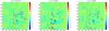 |
Fig. 5 Contours of the function α(x,y,z = 0). From left to right: Unpreprocessed, ppTW, and ppMF. The length unit is pixel (580 km) and α is measured in pixel-1. |
Absolute values of the differences between the preprocessed and observed fields.
In Table 3, the above metrics are given for the results of extrapolations using either the magnetofrictional relaxation method or the optimization method and starting from the observed magnetogram or a magnetogram that was preprocessed by ppTW or ppMF. It is seen in the table that for both extrapolation methods, only ppMF improves (i.e., makes smaller) the CWsin values of the calculated fields. On the other hand, their ⟨ |∇ B |/| B| ⟩ values are improved (i.e., brought closer to zero) for both extrapolation methods by both ppTW and ppMF. Similarly, the relative magnetic energy, ε, which is at unphysical values below 1 for the fields obtained by the extrapolations starting from the observed magnetogram, is raised to values larger than 1 for both extrapolation methods by both ppTW and ppMF. Additionally, we examined the average and maximum values of the Lorentz force in the extrapolation volume. ppMF leaves these values practically unchanged, while ppTW moderately increases them. This is largely in agreement with the results for the CWsin value, which stronger weights areas with a high current density.
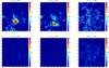 |
Fig. 6 Absolute values of the differences between the preprocessed and observed magnetograms for ppTW (top row) and ppMF (bottom row). From left to right: Differences for Bx, By, and Bz. The magnetic field is measured in G and the length unit is pixel (580 km). |
Figure 7,
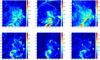 |
Fig. 7 Absolute value of current density, |∇ × B|, integrated vertically over a 12 pixel thick bottom layer, in G. Top row: Extrapolation with magnetofrictional method. Bottom row: Extrapolation with optimization method. From left to right: Unpreprocessed, ppTW, and ppMF. The length unit is pixel (580 km). |
finally, compares current densities for the six extrapolation/preprocessing cases in the form of |∇ × B| integrated vertically over a 12 pixel thick bottom region. For both extrapolations starting from the unpreprocessed vector magnetogram, the obtained current densities show very complex patterns.
In the case of the magnetofrictional extrapolation method (see Fig. 7, top row), the current density obtained when applying ppMF appears to be very similar to that for the case with no preprocessing. This means that ppMF here leads to a solution close to that obtained without preprocessing, but with a physical magnetic energy content and in better agreement with the force-free and solenoidal conditions (cf. Table 3). The field calculated by magnetofrictional extrapolation after applying ppTW, on the other hand, seems to be a much smoother and less structured version of the one calculated without preprocessing, at the same time being more physical in having an energy content in excess of the potential field value and in better fulfilling the solenoidal condition.
For the extrapolations using the optimization method (see Fig. 7, bottom row), the two preprocessing algorithms seem to have broadly similar effects on the current density. If one compares the cases with no preprocessing and with ppTW applied, one can again see that ppTW smoothes the current density strongly. In the case of preprocessing with ppMF the smoothing effect is also observable, though to a lesser degree. This may have to do with the fact that, independently of the kind of preprocessing applied, the current density distributions obtained by extrapolations with the optimization method show weaker contrasts than those obtained by magnetofrictional extrapolations. Comparing the figures in Table 3 from the point of view of the solutions’ consistency, we can see that the magnetofrictional extrapolations are closer to force-free (by a factor of three in CWsin), while the optimization method led to more solenoidal reconstructions. The optimization method is relatively little affected by the energy in the small scales of the unpreprocessed magnetogram, while the magnetofrictional method attained higher free energies with preprocessed magnetograms. (We do not extend further these observations since the comparison of different extrapolation techniques is not our subject here.)
4. Conclusions
We have compared and discussed the two so far existing methods for the preprocessing of solar vector magnetograms, namely, those of Wiegelmann et al. (2006b, ppTW and Fuhrmann et al. (2007, ppMF. These methods make the magnetograms more suitable for nonlinear force-free extrapolations into three-dimensional magnetic fields in the chromosphere and corona. Both methods follow the same strategy, namely, to minimize a functional L of the photospheric field values such as to simultaneously make small the total magnetic force and the total magnetic torque on the volume considered and the amount of small-scale noise in the photospheric boundary data.
The two methods differ in their ways of minimizing the functional L. While ppTW employs a Newton-Raphson scheme, ppMF uses the method of simulated annealing. Furthermore, the task of reducing the small-scale noise, or smoothing, is solved differently. ppTW applies a minimization of the absolute value of ΔB(x,y,z = 0), which corresponds to algebraically averaging the photospheric field, while in ppMF the smoothing is reached by a windowed-median averaging. Finally, the degree of deviation of the modified fields from the original photospheric field during the minimization is controlled in different ways by the two methods. In ppTW a special subfunctional that measures the deviation is included as an additional minimization target in L. This method of control is integral in character. ppMF, on the other hand, uses a local control at each grid point in the form of an interval within which the field values have to stay.
The two preprocessing methods were applied to a vector magnetogram of the recently observed active region NOAA AR 10 953, which had already been the target in a comparative study of different extrapolation methods for nonlinear force-free magnetic fields reported in DeRosa et al. (2009). Both preprocessing methods managed to significantly decrease the magnetic forces and magnetic torques that act through the magnetogram area and that can cause incompatibilities with the assumption of force-freeness in the solution domain. The force and torque decrease was stronger for ppMF than for ppTW.
Both methods also reduced the amount of small-scale irregularities in the observed photospheric field, where ppTW led to a markedly smoother magnetogram than ppMF, in accordance with the aim of ppTW to mimic the expansion of the solar magnetic field between photosphere and chromosphere. The average deviations of the preprocessed magnetograms from the observed magnetogram are nearly identical for ppTW and ppMF, where ppTW led to greater changes in strong-field areas, leaving weak-field areas mostly unchanged, while ppMF weakly changed the whole magnetogram, thereby better preserving patterns present in the original magnetogram. Similarly, for the function α(x,y,z = 0) ppTW yielded a much smoother distribution than ppMF.
The original magnetogram and the two preprocessed magnetograms were used as input data for nonlinear force-free field extrapolations by means of two different methods, namely the magnetofrictional relaxation method of Valori et al. (2007) and the optimization method of Wiegelmann (2004). Both ppTW and ppMF corrected a pathological property of the fields calculated by the extrapolations from the observed magnetogram, namely they raised the magnetic energy content of the extrapolated fields from values below to values above that for the potential field with the same normal component on the boundary. Also, the fields calculated from the preprocessed magnetograms fulfill the solenoidal condition for B better than those calculated without preprocessing. Finally, some effects of the preprocessing, as those on the current density in a bottom layer, seemed to be influenced by the the specifics of the employed extrapolation method.
Acknowledgments
Hinode is a Japanese mission developed and launched by ISAS/JAXA, with NAOJ as domestic partner and NASA and STFC (UK) as international partners. It is operated by these agencies in co-operation with ESA and NSC (Norway). M. Fuhrmann was supported by DFG grant SE 662/11-1 and T. Wiegelmann by DLR grant 50 OC 0501.
References
- Alissandrakis, C. E. 1981, A&A, 100, 197 [NASA ADS] [Google Scholar]
- Altschuler, M. D., & Newkirk, Jr., G. 1969, Sol. Phys., 9, 131 [Google Scholar]
- Aly, J. J. 1984, ApJ, 238, 349 [NASA ADS] [CrossRef] [Google Scholar]
- Aly, J. J. 1989, Sol. Phys., 120, 19 [NASA ADS] [CrossRef] [Google Scholar]
- Aly, J. J., & Seehafer, N. 1993, Sol. Phys., 144, 243 [NASA ADS] [CrossRef] [Google Scholar]
- Amari, T., Aly, J. J., Luciani, J. F., Boulmezaoud, T. Z., & Mikic, Z. 1997, Sol. Phys., 174, 129 [NASA ADS] [CrossRef] [Google Scholar]
- Amari, T., Boulmezaoud, T. Z., & Mikic, Z. 1999, A&A, 350, 1051 [NASA ADS] [Google Scholar]
- Amari, T., Boulmezaoud, T. Z., & Aly, J. J. 2006, A&A, 446, 691 [NASA ADS] [CrossRef] [EDP Sciences] [Google Scholar]
- Aschwanden, M. J., Wülser, J., Nitta, N. V., & Lemen, J. R. 2008, ApJ, 679, 827 [NASA ADS] [CrossRef] [Google Scholar]
- Bineau, M. 1972, Comm. Pure Appl. Math., 25, 77 [CrossRef] [Google Scholar]
- Boulmezaoud, T. Z., & Amari, T. 2000, Z. angew. Math. Phys., 51, 942 [CrossRef] [Google Scholar]
- Chiu, Y. T., & Hilton, H. H. 1977, ApJ, 212, 873 [NASA ADS] [CrossRef] [Google Scholar]
- Cuperman, S., Ofman, L., & Semel, M. 1990, A&A, 230, 193 [NASA ADS] [Google Scholar]
- Démoulin, P., Cuperman, S., & Semel, M. 1992, A&A, 263, 351 [NASA ADS] [Google Scholar]
- DeRosa, M. L., Schrijver, C. J., Barnes, G., et al. 2009, ApJ, 696, 1780 [Google Scholar]
- Fuhrmann, M., Seehafer, N., & Valori, G. 2007, A&A, 476, 349 [NASA ADS] [CrossRef] [EDP Sciences] [Google Scholar]
- Gary, G. A. 1989, ApJSS, 69, 323 [NASA ADS] [CrossRef] [EDP Sciences] [Google Scholar]
- Gary, G. A. 2001, Sol. Phys., 203, 71 [NASA ADS] [CrossRef] [Google Scholar]
- Golub, L., DeLuca, E., Austin, G., et al. 2007, Sol. Phys., 243, 63 [NASA ADS] [CrossRef] [Google Scholar]
- Grad, H., & Rubin, H. 1958, in Proc. 2nd Int. Conf. Peaceful Uses of Atomic Energy, 31 (Geneva: United Nations), 190 [Google Scholar]
- He, H., & Wang, H. 2006, MNRAS, 369, 207 [NASA ADS] [CrossRef] [Google Scholar]
- Howard, R. A., Moses, J. D., Vourlidas, A., et al. 2008, Space Sci. Rev., 136, 67 [NASA ADS] [CrossRef] [Google Scholar]
- Jing, J., Tan, C., Yuan, Y., et al. 2010, ApJ, 713, 440 [NASA ADS] [CrossRef] [Google Scholar]
- Kaiser, R., Neudert, M., & von Wahl, W. 2000, Commun. Math. Phys., 211, 111 [NASA ADS] [CrossRef] [Google Scholar]
- Kano, R., Sakao, T., Hara, H., et al. 2008, Sol. Phys., 249, 263 [NASA ADS] [CrossRef] [Google Scholar]
- Kosugi, T., Matsuzaki, K., Sakao, T., et al. 2007, Sol. Phys., 243, 3 [NASA ADS] [CrossRef] [Google Scholar]
- Lites, B. W., Low, B. C., Martínez Pillet, V., et al. 1995, ApJ, 446, 877 [NASA ADS] [CrossRef] [Google Scholar]
- Low, B. C. 1985, in Measurements of Solar Vector Magnetic Fields, ed. M. J. Hagyard, NASA Conf. Publ., 2374, 49 [Google Scholar]
- Low, B. C., & Lou, Y. Q. 1990, ApJ, 352, 343 [NASA ADS] [CrossRef] [Google Scholar]
- McClymont, A. N., Jiao, L., & Mikić, Z. 1997, Sol. Phys., 174, 191 [NASA ADS] [CrossRef] [Google Scholar]
- Metcalf, T. R., Leka, K. D., Barnes, G., et al. 2006, Sol. Phys., 237, 267 [Google Scholar]
- Metcalf, T. R., DeRosa, M. L., Schrijver, C. J., et al. 2007, Proc. 210th Meeting American Astrononomical Society, Honolulu, Hawaii, 27–31 May, BAAS, 39, 091.02 [Google Scholar]
- Metcalf, T. R., DeRosa, M. L., Schrijver, C. J., et al. 2008, Sol. Phys., 247, 269 [Google Scholar]
- Mikic, Z., & McClymont, A. N. 1994, in Solar Active Region Evolution: Comparing Models with Observations, ed. K. S. Balasubramaniam, & G. W. Simon (San Francisco: ASP), ASP Conf. Ser., 68, 225 [Google Scholar]
- Molodenskii, M. M. 1969, Sov. Astron. AJ, 12, 585 [Google Scholar]
- Nakagawa, Y., & Raadu, M. A. 1972, Sol. Phys., 25, 127 [NASA ADS] [CrossRef] [Google Scholar]
- Okamoto, T. J., Tsuneta, S., Lites, B. W., et al. 2008, ApJ, 673, L215 [NASA ADS] [CrossRef] [Google Scholar]
- Press, W. H., Flannery, B. P., Teukolsky, S. A., & Vetterling, W. T. 1989, Numerical Recipes. The Art of Scientific Computing (Cambridge, UK: Cambridge University Press) [Google Scholar]
- Roumeliotis, G. 1996, ApJ, 473, 1095 [NASA ADS] [CrossRef] [Google Scholar]
- Sakurai, T. 1981, Sol. Phys., 69, 343 [NASA ADS] [CrossRef] [Google Scholar]
- Sakurai, T. 1989, Space Sci. Rev., 51, 11 [NASA ADS] [Google Scholar]
- Schatten, K. H., Wilcox, J. M., & Ness, N. F. 1969, Sol. Phys., 6, 442 [Google Scholar]
- Scherrer, P. H., Bogart, R. S., Bush, R. I., et al. 1995, Sol. Phys., 162, 129 [Google Scholar]
- Schmidt, H. U. 1964, in AAS/NASA Symp. Physics of Solar Flares, ed. W. N. Hess, NASA Sp. Publ. No. SP-50 (Washington, D.C.: NASA), 107 [Google Scholar]
- Schrijver, C. J., DeRosa, M. L., Metcalf, T. R., et al. 2006, Sol. Phys., 235, 161 [Google Scholar]
- Schrijver, C. J., DeRosa, M. L., Metcalf, T., et al. 2008, ApJ, 675, 1637 [Google Scholar]
- Seehafer, N. 1978, Sol. Phys., 58, 215 [NASA ADS] [CrossRef] [Google Scholar]
- Seehafer, N. 1982, Sol. Phys., 81, 69 [NASA ADS] [CrossRef] [Google Scholar]
- Seehafer, N., & Staude, J. 1983, Phys. Solariterr., 22, 5 [Google Scholar]
- Semel, M. 1988, A&A, 198, 293 [NASA ADS] [Google Scholar]
- Song, M. T., Fang, C., Tang, Y. H., Wu, S. T., & Zhang, Y. A. 2006, ApJ, 649, 1084 [NASA ADS] [CrossRef] [Google Scholar]
- Su, Y., van Ballegooijen, A., Lites, B. W., et al. 2009, ApJ, 691, 105 [NASA ADS] [CrossRef] [Google Scholar]
- Tadesse, T., Wiegelmann, T., & Inhester, B. 2009, A&A, 508, 421 [NASA ADS] [CrossRef] [EDP Sciences] [Google Scholar]
- Teuber, D., Tandberg-Hanssen, E., & Hagyard, M. J. 1977, Sol. Phys., 53, 97 [NASA ADS] [CrossRef] [Google Scholar]
- Titov, V. S., & Démoulin, P. 1999, A&A, 351, 707 [NASA ADS] [Google Scholar]
- Tsuneta, S., Ichimoto, K., Katsukawa, Y., et al. 2008, Sol. Phys., 249, 167 [NASA ADS] [CrossRef] [Google Scholar]
- Valori, G., Kliem, B., & Keppens, R. 2005, A&A, 433, 335 [NASA ADS] [CrossRef] [EDP Sciences] [Google Scholar]
- Valori, G., Kliem, B., & Fuhrmann, M. 2007, Sol. Phys., 245, 263 [NASA ADS] [CrossRef] [Google Scholar]
- Valori, G., Kliem, B., Török, T., & Titov, V. S. 2010, A&A, 519, A44 [NASA ADS] [CrossRef] [EDP Sciences] [Google Scholar]
- Wheatland, M. S. 2004, Sol. Phys., 222, 247 [NASA ADS] [CrossRef] [Google Scholar]
- Wheatland, M. S. 2006, Sol. Phys., 238, 29 [NASA ADS] [CrossRef] [Google Scholar]
- Wheatland, M. S., Sturrock, P. A., & Roumeliotis, G. 2000, ApJ, 540, 1150 [Google Scholar]
- Wiegelmann, T. 2004, Sol. Phys., 219, 87 [NASA ADS] [CrossRef] [Google Scholar]
- Wiegelmann, T. 2007, Sol. Phys., 240, 227 [NASA ADS] [CrossRef] [Google Scholar]
- Wiegelmann, T. 2008, J. Geophys. Res., 113, A03S02 [Google Scholar]
- Wiegelmann, T., Inhester, B., Kliem, B., Valori, G., & Neukirch, T. 2006a, A&A, 453, 737 [NASA ADS] [CrossRef] [EDP Sciences] [Google Scholar]
- Wiegelmann, T., Inhester, B., & Sakurai, T. 2006b, Sol. Phys., 233, 215 [NASA ADS] [CrossRef] [Google Scholar]
- Wiegelmann, T., Thalmann, J. K., Schrijver, C. J., De Rosa, M. L., & Metcalf, T. R. 2008, Sol. Phys., 247, 249 [NASA ADS] [CrossRef] [Google Scholar]
- Wu, S. T., Chang, H. M., & Hagyard, M. J. 1985, in NASA Conf. Publ., 2374, Measurements of Solar Vector Magnetic Fields, ed. M. J. Hagyard, 17 [Google Scholar]
- Wu, S. T., Sun, M. T., Chang, H. M., Hagyard, M. J., & Gary, G. A. 1990, ApJ, 362, 698 [NASA ADS] [CrossRef] [Google Scholar]
- Yan, Y. 2003, Space Sci. Rev., 107, 119 [NASA ADS] [CrossRef] [Google Scholar]
- Yan, Y., & Li, Z. 2006, ApJ, 638, 1162 [NASA ADS] [CrossRef] [Google Scholar]
- Yan, Y., & Sakurai, T. 1997, Sol. Phys., 174, 65 [NASA ADS] [CrossRef] [Google Scholar]
- Yan, Y., & Sakurai, T. 2000, Sol. Phys., 195, 89 [NASA ADS] [CrossRef] [Google Scholar]
- Yang, W. H., Sturrock, P. A., & Antiochos, S. K. 1986, ApJ, 309, 383 [NASA ADS] [CrossRef] [Google Scholar]
All Tables
All Figures
|
Fig. 1 Two coaligned images of AR 10 953 (with the same 10 degree gridlines drawn on both images for reference). a) Time-averaged and logarithmically scaled Hinode/XRT soft X-ray image; and b) STEREO-A/SECCHI-EUVI 171 Å image. |
| In the text | |
|
Fig. 2 Original and preprocessed vector magnetograms of AR 10 953. From left to right: Bx, By, and Bz. From top to bottom: Unpreprocessed, ppTW, and ppMF. The magnetic field is measured in G and the length unit is pixel (580 km). |
| In the text | |
|
Fig. 3 By in a magnified cutout of the vector magnetogram of AR10 953. From left to right: Unpreprocessed, ppTW, and ppMF. The magnetic field is measured in G and the length unit is pixel (580 km). |
| In the text | |
|
Fig. 4 Evolution of the total functional L(MF) as given by
Eq. (20) (top)
and of the sum |
| In the text | |
|
Fig. 5 Contours of the function α(x,y,z = 0). From left to right: Unpreprocessed, ppTW, and ppMF. The length unit is pixel (580 km) and α is measured in pixel-1. |
| In the text | |
|
Fig. 6 Absolute values of the differences between the preprocessed and observed magnetograms for ppTW (top row) and ppMF (bottom row). From left to right: Differences for Bx, By, and Bz. The magnetic field is measured in G and the length unit is pixel (580 km). |
| In the text | |
|
Fig. 7 Absolute value of current density, |∇ × B|, integrated vertically over a 12 pixel thick bottom layer, in G. Top row: Extrapolation with magnetofrictional method. Bottom row: Extrapolation with optimization method. From left to right: Unpreprocessed, ppTW, and ppMF. The length unit is pixel (580 km). |
| In the text | |
Current usage metrics show cumulative count of Article Views (full-text article views including HTML views, PDF and ePub downloads, according to the available data) and Abstracts Views on Vision4Press platform.
Data correspond to usage on the plateform after 2015. The current usage metrics is available 48-96 hours after online publication and is updated daily on week days.
Initial download of the metrics may take a while.