© ESO, 2011

1. Introduction

At the present time, the general belief is that supermassive black holes (SMBHs) located at the centre of galaxies have been formed by the growth of primordial “seeds” either by matter accretion or coalescences during merger episodes. This picture is consistent with how the present black hole (BH) mass density compares quite well with the mass density derived from the bolometric luminosity function of quasars, under the assumption that the accretion process itself is the source of the radiated energy (Soltan 1982; Small & Blandford 1992; Hopkins et al. 2007). The accreted matter is essentially baryonic in origin with an eventual contribution from the exotic dark component not exceeding 10% of the total accreted matter (Peirani & de Freitas Pacheco 2008).

Nevertheless, the formation of massive BHs by the direct collapse of central regions of proto-galaxies is an alternative possibility considered by different authors. Shapiro (2004) considered the core collapse of relativistic star clusters formed in starbursts, which may have occurred in the early evolution of galaxies. The collapse of a collisionless system, once it has experienced a phase of strong oscillations followed by violent relaxation, may undergo a slow gravothermal instability, if the phase-space incompressibility condition is violated (Levin et al. 2008), leading eventually to the formation of a BH. Despite not including the star formation process and its associated feedback, Wise et al. (2009) find from hydrodynamical simulations of  ~10⁸ M_⊙ proto-galaxies, that massive central objects with masses around 10⁵ M_⊙ could form inside regions of one parsec radius. The most favourable physical conditions for the gas in these proto-halos to form those massive central objects are when the virial temperature is about 15 000 K and the circular velocity around 20 km s^-1 (Reagan & Haehnelt 2009).

If the aforementioned investigations open the possibility of directly forming massive BH via the gravitational collapse, other studies lead to the formation of intermediate mass BH, which could be the required seeds. Black holes in the mass range (10³−10⁴ M_⊙) could be formed by the collapse of primordial gas clouds (Haehnelt & Rees 1993; Eisenstein & Loeb 1995; Koushiappas et al. 2004). Another appealing possibility, which is considered in the present investigation, is the formation of BH seeds with masses in the range 10²−10⁴ M_⊙, resulting from the evolution of primordial massive stars (Bromm et al. 1999; Abel et al. 2000; Heger et al. 2003; Yoshida et al. 2006). These stars would have been formed at z ~ 15−20 in the high-density peaks of the primordial fluctuation spectrum (Gao et al. 2007), and their high masses would be the consequence of very inefficient gas cooling at zero metallicity. Besides forming BH seeds, these massive stars could also have contributed to the reionization of the universe.

Different investigations based on cosmological simulations have been performed in these past years, aiming to understand the growth process of seeds, the consequences of the feedback resulting from the accretion process itself on the environment, and the observed correlations between the black hole mass with properties of the host galaxy (DiMatteo et al. 2003; Pelupessy et al. 2007; Springel et al. 2005; Filloux et al. 2010). In all these simulations, the physical description of the accretion process requires a substantial simplification, since it occurs on unresolved spatial scales. If the BH is at rest with respect to the gas, the inflow is probably spherical, or almost adiabatic, and the accretion rate is estimated by the Hoyle-Lyttleton-Bondi (HLB) formula (Hoyle & Lyttleton 1939; Bondi & Hoyle 1944), whose rate depends on parameters such as the gas density and the sound velocity evaluated far away from the BH, on scales supposed to be resolved by simulations. The assumption that BHs could be at rest and that the accretion process is spherically symmetric is probably unrealistic but frequently used in cosmological simulations due to its simplicity. However, the radiation emitted during the inflow, in particular near the BH horizon, affects the surrounding gas, considerably reducing the accretion rate and rendering the growth of seeds by such a mechanism inefficient (Milosavljevic et al. 2009). The situation is rather different if the BH is moving with respect to the gas. After passing the BH, a conically shaped shock is produced in the flow, where the gas loses the momentum component perpendicular to the shock front. After compression in the shock, gas particles within a certain impact parameter will fall into the black hole. Particles having angular momentum exceeding 2r_gc, with r_g the gravitational radius, will form a disk, and only after viscous stresses have transported away the excess of angular momentum will the gas cross the BH horizon. Clearly, all these processes are not adequately described in any of the aforementioned simulations and one may wonder whether the accretion or the resulting luminosity is estimated satisfactorily when the Hoyle-Lyttleton-Bondi approach is adopted.

Numerical simulations indicate that, after the merger of two galaxies, a considerable amount of gas is settled into the central region of the resulting object. The gas loses angular momentum on a timescale comparable to the dynamical timescale, forming a circumnuclear self-gravitating disk (Mihos & Hernquist 1996; Barnes 2002), which have masses in the range 10⁶−10⁹ M_⊙ and dimensions of about 100−500 pc. Such a disk will probably be able to feed the central BH, increasing its mass. In fact, this scenario was considered by Filloux et al. (2010) in their simulations. These authors adopted an accretion rate derived from a steady disk model, in which the angular momentum transport is provided by turbulent viscosity. Since in reality the disk is expected not to be steady, they assumed that during a time step the properties of the disk do not change appreciably, but they are updated continuously at each new time step. Despite this simple description of the accretion process, they were able to reproduce the main properties of BHs and their host galaxies quite satisfactory. More recently, Power et al. (2011) have introduced a new method of modelling the physics of an accreting disk around a BH, which has some common points with the approach by Filloux et al. (2010). Based on a series of numerical experiments, they have shown that the disk accretion mode is more physically consistent than the simple use of the HLB formula and more efficient at feeding the seed, in agreement with the conclusions by Filloux et al. (2010). In these last two approaches, the accretion disk is represented in simulations by a “single” (or two in rare cases) SPH particle and the adopted prescription for the accretion rate defines the mass fraction transferred to the central BH. In the real world, the structure of the disk changes continuously for different reasons: mass is transferred either to the central BH or to the outskirts of the disk, stars form by consuming part of gas available to feed the BH, and infall of matter is a source of fresh gas replenishing the disk.

The understanding of the aforementioned aspects require close inspection of the accretion process to improve the modellization adopted in cosmological simulations. In the present paper we report results of the numerical solution of the hydrodynamic equations describing the evolution of a circumnuclear disk around a black hole, in an attempt to answer some specific questions that could be useful for improving the modelling of such a process in cosmological simulations. Moreover, SLOAN quasars associated to very massive BHs (Fan et al. 2001; Willot et al. 2003) have already been observed at redshifts z ~ 6, when the universe was only 0.96 Gyr old. These observations imply that the growth process of seeds should occur on shorter timescales, in regions where the accretion mechanism must be very efficient. The present investigation mainly focuses on the following questions: 1) what is the fraction of the disk mass accreted by the central BH? 2) Does such a fraction depend on the initial mass either of the BH seed or the disk? 3) What are the typical accretion timescales and how do they depend on the disk parameters? This paper is organized as follows. In Sect. 2 the accretion disk model is discussed and the main equations are introduced. In Sect. 3 the numerical methods are presented. In Sect. 4 the main results are given; finally, in Sect. 5 the conclusions are summarized.

2. The accretion disk model

In this work, we will study the evolution of nuclear disks formed possibly after a merger event or by gas infall, having masses in the range 10⁷−10⁸ M_⊙ and with typical dimensions of the order of 50 pc. These disks are initially self-gravitating and, as the central BH grows, it dominates the dynamics of the inner regions while the outer parts are still dominated by the disk self gravitation. As we shall see later, the external disk is comprised of neutral gas having temperatures of about 100–2000 K, conditions favourable to forming stars. However, in the present work, the gas conversion into stars through the disk will not be considered, although a new version of our code, presently under development, will offer such a possibility.

2.1. Angular momentum transport

A major problem in the current understanding of accretion disks is the absence of a physical theory able to describe the viscosity of the gas in the presence of either turbulent flows or a magnetic field. The angular momentum transport in accretion disks is generally described by the formalism introduced almost forty years ago by Shakura & Sunyaev (1973), in which the viscosity due to the subsonic turbulence is parametrized by the relation $\mathit{\eta }\mathrm{=}\mathit{\alpha H}{\mathit{c}}_{\mathrm{s}}\mathit{,}$(1)where α ≤ 1 is a dimensionless coefficient, H the vertical scale of the disk supposed to be of the same order as the typical (isotropic) turbulence scale ℓ_t, and c_s the sound velocity. Accretion disk models based on the “α-viscosity” approach are able to successfully explain the observed properties of dwarf-novae and X-ray binaries, but disks based on such a formulation are thermally unstable as demonstrated long ago by Piran (1978).

The possibility that turbulence could be generated by local gravitational instability in geometrically thin disks was considered by Paczynski (1978). Duschl & Britsch (2006) revisited this idea by analysing the gravitational instability of self-gravitating disks, concluding that such an instability could be able to develop turbulence in the flow and, consequently, to generate viscosity without requiring the contribution of magneto-hydrodynamic turbulence. Recent simulations of the gas inflow in the central regions of galaxies, induced by the gravitational potential either of the stellar nucleus or the SMBH, reveal the appearance of highly supersonic turbulence, with velocities clsoe to the virial value (Regan & Haehenelt 2009; Levine et al. 2008; Wise et al. 2008). Amazingly, no fragmentation is observed in such a gas despite being isothermal and gravitationally unstable. In fact, Begelman & Shlosman (2009) argue that an efficient angular momentum transfer suppresses fragmentation, favouring the gas inflow. In contrast, if the angular momentum transfer is inefficient, the turbulence decays and triggers global instabilities, which in turn regenerates a turbulent flow. Moreover, according to their analysis, fragmentation is suppressed whenever the gas temperature remains below the virial value. As we shall see later, during the early evolutionary phases of the disk, the accretion rate is quite important. Consequently, the heat generated by dissipation of turbulence increases the radiation pressure, which inflates the inner regions, thereby producing a “slim” disk. We would expect that a flow self-regulated by this mechanism could be stable against fragmentation. If the flow is self-regulated, it must be characterized by a critical Reynolds number ℛ, determined by the viscosity below which the flow becomes unstable. De Freitas Pacheco & Steiner (1976) suggested that instead of the “α” parametrization, the effective (turbulent) viscosity η could be expressed in terms of such a critical Reynolds number by $\mathit{\eta }\mathrm{=}\frac{\mathrm{2}\mathit{\pi r}{\mathit{V}}_{\mathit{\phi }}}{\mathrm{ℛ}}\mathit{,}$(2)where r is the radial distance to the centre of the disk (or to the central BH) and V_φ = Ωr is the azimuthal velocity of the gas. It is worth mentioning that this formulation, which is adopted here, is essentially the “β-viscosity” model discussed by Duschl et al. (1998; see also Richard & Zahn 1999). An additional aspect justifying adoption of this formulation is that accretion disks modeled by such a viscosity prescription are thermally stable according to the analysis by Piran (1978). However, in the present work the disk stability was not investigated and we cannot exclude the possibility that fragmentation occurs. This aspect will be examined in a future paper.

It can be verified easily that the Mach number associated to the mean turbulent motions is ${\mathit{M}}_{\mathrm{t}}\mathrm{\simeq }{\mathit{V}}_{\mathit{\phi }}\mathit{/}\mathrm{\left(}{\mathit{c}}_{\mathrm{s}}\sqrt{\mathrm{ℛ}}\mathrm{\right)}$ in such a formulation. This implies that turbulence is slightly supersonic in most regions of the disk, but it can be supersonic in the inner regions, depending on the critical Reynolds number.

2.2. The dynamical equations

The hydrodynamic equations are written in cylindrical coordinates (r,φ,z) and, in order to simplify the solution of the Poisson equation, variables are integrated along the z-axis but the scale of height is calculated in a consistent way as seen below. The equation of the radial motion, neglecting gas pressure gradients, is $\frac{\mathit{\partial }{\mathit{V}}_{\mathit{r}}}{\mathit{\partial t}}\mathrm{+}{\mathit{V}}_{\mathit{r}}\frac{\mathit{\partial }{\mathit{V}}_{\mathit{r}}}{\mathit{\partial r}}\mathrm{-}\frac{{\mathit{V}}_{\mathit{\phi }}^{\mathrm{2}}}{\mathit{r}}\mathrm{-}\frac{\mathit{\partial \psi }}{\mathit{\partial r}}\mathrm{=}\mathrm{0}\mathit{,}$(3)where V_r is the radial velocity, V_φ the azimuthal velocity, and ψ the gravitational potential, including the contribution of the central BH and of the disk itself. The central BH is probably rotating, but in the present investigation we discard this possibility and use the approximate potential of Paczyński-Wiita (Paczyński & Wiita 1980) to model the gravitational field of the BH. The contribution of the disk itself is obtained from the expression for the internal potential of an ellipsoid in which we have performed the limit z → 0. Under these conditions the total gravitational force is $\frac{\mathit{\partial \psi }}{\mathit{\partial r}}\mathrm{=}\mathrm{-}\frac{\mathit{G}{\mathit{M}}_{\mathrm{BH}}\mathrm{\left(}\mathit{t}\mathrm{\right)}}{\mathrm{(}\mathit{r}\mathrm{-}{\mathit{r}}_{\mathrm{g}}{\mathrm{)}}^{\mathrm{2}}}\mathrm{-}\frac{\mathit{G}}{\mathit{r}}{\mathrm{\int }}_{\mathrm{0}}^{\mathit{r}}\frac{\mathrm{\Sigma }\mathrm{\left(}\mathit{a,t}\mathrm{\right)}\mathit{a}\mathrm{d}\mathit{a}}{\sqrt{{\mathit{r}}^{\mathrm{2}}\mathrm{-}{\mathit{a}}^{\mathrm{2}}}}\mathit{,}$(4)where r_g = 2GM_BH/c² is the gravitational (or the event horizon) radius and Σ the columnar mass density defined by $\mathrm{\Sigma }\mathrm{\left(}\mathit{r,t}\mathrm{\right)}\mathrm{=}{\mathrm{\int }}_{\mathrm{-}\mathrm{\infty }}^{\mathrm{\infty }}\mathit{\rho }\mathrm{\left(}\mathit{r,z,t}\mathrm{\right)}\mathrm{d}\mathit{z}\mathit{.}$(5)The mass of the BH varies according to the equation $\frac{\mathrm{d}{\mathit{M}}_{\mathrm{BH}}\mathrm{\left(}\mathit{t}\mathrm{\right)}}{\mathrm{d}\mathit{t}}\mathrm{=}\mathrm{2}\mathit{\pi }{\mathit{r}}_{\mathrm{lso}}\mathrm{\left(}\mathit{t}\mathrm{\right)}\mathrm{\Sigma }\mathrm{\left(}{\mathit{r}}_{\mathrm{lso}}\mathit{,t}\mathrm{\right)}{\mathit{V}}_{\mathit{r}}\mathrm{\left(}{\mathit{r}}_{\mathrm{lso}}\mathit{,t}\mathrm{\right)}\mathit{,}$(6)where the quantities on the right side are evaluated at the radius of the last stable circular orbit r_lso. As the BH grows, the radius of the horizon and of the last stable circular orbit increase proportionally to the BH mass.

The continuity equation is given by $\frac{\mathit{\partial }\mathrm{\Sigma }}{\mathit{\partial t}}\mathrm{+}\frac{\mathrm{1}}{\mathit{r}}\frac{\mathit{\partial }\mathrm{\left(}\mathit{r}\mathrm{\Sigma }{\mathit{V}}_{\mathit{r}}\mathrm{\right)}}{\mathit{\partial r}}\mathrm{=}\mathrm{0}\mathit{,}$(7)and the equation for the azimuthal motion, including the viscous forces responsible for the angular momentum transport is $\frac{\mathit{\partial }{\mathit{V}}_{\mathit{\phi }}}{\mathit{\partial t}}\mathrm{+}{\mathit{V}}_{\mathit{r}}\frac{\mathit{\partial }{\mathit{V}}_{\mathit{\phi }}}{\mathit{\partial r}}\mathrm{+}\frac{{\mathit{V}}_{\mathit{r}}{\mathit{V}}_{\mathit{\phi }}}{\mathit{r}}\mathrm{+}\frac{\mathrm{1}}{\mathit{r}\mathrm{\Sigma }}\frac{\mathit{\partial }\mathrm{\left(}\mathit{r}{\mathit{T}}_{\mathit{r\phi }}\mathrm{\right)}}{\mathit{\partial r}}\mathrm{=}\mathrm{0}\mathit{,}$(8)where the considered component of the stress tensor (integrated along the z-axis) is ${\mathit{T}}_{\mathit{r\phi }}\mathrm{=}\mathit{\eta }\mathrm{\Sigma }\mathit{r}\frac{\mathit{\partial }\mathrm{\Omega }}{\mathit{\partial r}}\mathrm{·}$(9)Using Eq. (2), the equation above can be recast as ${\mathit{T}}_{\mathit{r\phi }}\mathrm{=}\left(\frac{\mathrm{2}\mathit{\pi }}{\mathrm{ℛ}}\right)\mathrm{\Sigma }{\mathit{r}}^{\mathrm{3}}\mathrm{\Omega }\frac{\mathit{\partial }\mathrm{\Omega }}{\mathit{\partial r}}\mathrm{·}$(10)

2.3. The scale of height

Assuming that the disk is in hydrostatic equilibrium along the z-axis, we can write $\frac{\mathrm{d}\mathrm{(}{\mathit{P}}_{\mathrm{g}}\mathrm{+}{\mathit{P}}_{\mathrm{t}}\mathrm{+}{\mathit{P}}_{\mathrm{r}}\mathrm{)}}{\mathrm{d}\mathit{z}}\mathrm{=}\mathrm{-}\mathit{\rho }{\mathit{g}}_{\mathit{z}}\mathit{,}$(11)where ${\mathit{P}}_{\mathrm{g}}\mathrm{=}\mathit{\rho }{\mathit{c}}_{\mathrm{s}}^{\mathrm{2}}$, ${\mathit{P}}_{\mathrm{t}}\mathrm{=}\mathit{\rho }\mathrm{⟨}{\mathit{v}}_{\mathrm{t}}^{\mathrm{2}}\mathrm{⟩}$, and P_r = aT⁴/3 are the gas the turbulent and the radiation pressure, respectively. The vertical component of the gravitational acceleration makes two contributions: one from the disk self-gravity and another from the tidal force due to the central black hole. Thus, ${\mathit{g}}_{\mathit{z}}\mathrm{=}\mathrm{2}\mathit{\pi G}\mathrm{\Sigma }\frac{\mathit{z}}{\mathit{H}}\mathrm{+}\frac{\mathit{G}{\mathit{M}}_{\mathrm{BH}}}{{\mathit{r}}^{\mathrm{3}}}\mathit{z}\mathit{.}$(12)Defining an effective scale of height by the relation H = ρ/(| dρ/dz|) and using the equations above, one obtains, after some algebra, $\mathit{H}\mathrm{=}\mathrm{-}\frac{{\mathit{c}}_{\mathrm{s}}}{\mathit{Q̅}{\mathrm{\Omega }}_{\mathrm{K}}}\left[\mathrm{(}\mathrm{1}\mathrm{-}\mathit{\beta }\mathrm{)}\mathrm{-}\sqrt{\mathrm{(}\mathrm{1}\mathrm{-}\mathit{\beta }{\mathrm{)}}^{\mathrm{2}}\mathrm{+}\mathit{Q̅}\mathrm{2}\mathrm{(}\mathrm{1}\mathrm{+}{\mathit{\epsilon }}^{\mathrm{2}}\mathrm{)}}\right]\mathit{,}$(13)where ${\mathit{\epsilon }}^{\mathrm{2}}\mathrm{=}\mathrm{⟨}{\mathit{v}}_{\mathrm{t}}^{\mathrm{2}}\mathrm{⟩}\mathit{/}{\mathit{c}}_{\mathrm{s}}^{\mathrm{2}}$, and we have introduced ${\mathrm{\Omega }}_{\mathrm{K}}^{\mathrm{2}}\mathrm{=}\frac{\mathit{G}{\mathit{M}}_{\mathrm{BH}}}{{\mathit{r}}^{\mathrm{3}}}\mathit{,}$(14)and $\mathit{Q̅}\mathrm{=}\frac{{\mathrm{\Omega }}_{\mathrm{K}}{\mathit{c}}_{\mathrm{s}}}{\mathit{\pi G}\mathrm{\Sigma }}\mathrm{·}$(15)The parameter β, defined as $\mathit{\beta }\mathrm{=}\frac{\mathit{a}{\mathit{T}}^{\mathrm{4}}}{\mathrm{3}\mathit{\pi G}{\mathrm{\Sigma }}^{\mathrm{2}}}\mathit{,}$(16)measures the ratio between the radiation pressure and the disk self-gravity. Some limiting cases can be derived from Eq. (13). When the radiation force is insignificant (β ≪ 1) and self-gravity dominates (), one obtains $\mathit{H}\mathrm{\simeq }\frac{{\mathit{c}}_{\mathrm{s}}^{\mathrm{2}}\mathrm{(}\mathrm{1}\mathrm{+}{\mathit{\epsilon }}^{\mathrm{2}}\mathrm{)}}{\mathrm{2}\mathit{\pi G}\mathrm{\Sigma }}\mathit{,}$(17)whereas when , namely, the vertical acceleration is dominated by tidal forces, we have $\mathit{H}\mathrm{\simeq }\frac{{\mathit{c}}_{\mathrm{s}}\sqrt{\mathrm{(}\mathrm{1}\mathrm{+}{\mathit{\epsilon }}^{\mathrm{2}}\mathrm{)}}}{{\mathrm{\Omega }}_{\mathrm{K}}}\mathrm{·}$(18)It is worth mentioning that when the disk becomes optically thin, the contribution by the radiation pressure is negligible and, in this case, the scale of height is computed from Eq. (13) with the condition β = 0.

2.4. The temperature of the disk

We assume that all energy is generated locally by viscous dissipation and radiated essentially along the z-axis, although a small fraction could be advected inwards. Under these conditions, the local energy balance is given by ${\mathit{Q}}_{\mathrm{dis}}\mathrm{=}{\mathit{Q}}_{\mathrm{rad}}\mathrm{+}{\mathit{Q}}_{\mathrm{adv}}\mathit{.}$(19)The energy rate per unit of area dissipated by viscous forces is ${\mathit{Q}}_{\mathrm{dis}}\mathrm{=}\frac{\mathrm{2}\mathit{\pi }}{\mathrm{ℛ}}\mathrm{\Sigma }{\mathrm{\Omega }}^{\mathrm{3}}{\mathit{r}}^{\mathrm{2}}{\left(\frac{\mathrm{d}\lg \mathrm{\Omega }}{\mathrm{d}\lg \mathit{r}}\right)}^{\mathrm{2}}\mathit{,}$(20)while the advected energy flux is (Abramowicz et al. 1986) ${\mathit{Q}}_{\mathrm{adv}}\mathrm{=}\mathit{f}\mathrm{\left(}\mathit{r}\mathrm{\right)}{\left(\frac{\mathit{H}}{\mathit{r}}\right)}^{\mathrm{2}}{\mathit{Q}}_{\mathrm{dis}}\mathit{,}$(21)where f(r) depends on the angular momentum distribution throughout the disk, but in general, it is close to the unity (Abramowicz et al. 1995), except near the star-disk transition layer, where it could attain very high values. In our case, since the central object is a black hole, such a layer does not exist and the f(r) factor depends on the difference between the angular momentum at the considered position and at the last stable orbit. Here we simply assume that f(r) = 1 everywhere in the disk.

In the regions where the disk is partially or completely ionized, the opacity is due to the Thomson scattering, bound-free, and free-free transitions. In this case, when using the solution of the transfer equation within the Eddington approximation derived by de Freitas Pacheco et al. (1977), the local emergent flux is ${\mathrm{\Phi }}_{\mathit{\nu }}\mathrm{\left(}{\mathit{T}}_{\mathrm{e}}\mathrm{\right(}\mathit{r}\mathrm{\left)}\mathrm{\right)}\mathrm{\simeq }\frac{\mathrm{2}\mathit{\pi }{\mathit{B}}_{\mathit{\nu }}\mathrm{\left(}{\mathit{T}}_{\mathrm{e}}\mathrm{\right)}}{\left[\mathrm{1}\mathrm{+}\frac{\sqrt{\mathrm{3}}}{\mathrm{2}{\mathit{\lambda }}_{\mathit{\nu }}}\coth {\mathit{t}}_{\mathrm{0}\mathit{,\nu }}\right]}\mathit{,}$(22)where ${\mathit{t}}_{\mathrm{0}\mathit{,\nu }}\mathrm{=}\sqrt{\mathrm{3}{\mathit{\tau }}_{\mathrm{f}}{}^{\mathrm{(}}\mathit{\tau }_{\mathrm{f}}\mathrm{+}{\mathit{\tau }}_{\mathrm{s}}{}^{\mathrm{)}}}$ is the effective optical depth, with τ_f and τ_s the absorption and scattering optical depths, respectively. The other parameter is defined by the relation ${\mathit{\lambda }}_{\mathit{\nu }}^{\mathrm{2}}\mathrm{=}{\mathit{\tau }}_{\mathrm{f}}\mathit{/}\mathrm{(}{\mathit{\tau }}_{\mathrm{f}}\mathrm{+}{\mathit{\tau }}_{\mathrm{s}}\mathrm{)}$ and T_e is the effective temperature. Thus, ${\mathit{Q}}_{\mathrm{rad}}\mathrm{=}\mathrm{2}{\mathrm{\int }}_{\mathrm{0}}^{\mathrm{\infty }}{\mathrm{\Phi }}_{\mathit{\nu }}\mathrm{\left(}{\mathit{T}}_{\mathrm{e}}\mathrm{\right(}\mathit{r}\mathrm{\left)}\mathrm{\right)}\mathrm{d}\mathit{\nu ,}$(23)where the factor 2 takes into account both disk surfaces.

Another factor in the evaluation of the disk temperature is photon trapping. At very high optical depths, the photon diffusion timescale along the z-axis t_d = 3(H/c)t₀ can be larger than the accretion timescale t_ac = r/V_r. Here t₀ is the frequency averaged effective optical depth as defined above. When this occurs, photons are not able to reach the surface, because they are inwards and swallowed by the central BH. In this case, besides the advection correction, the dissipated energy should be reduced by an extra factor equal to the ratio t_ac/t_d.

The local effective temperature is derived from the numerical solution of these equations. In the outer regions, the disk is neutral and optically thin. In this case, the temperature was estimated simply from the balance between the heating and the cooling rates. The cooling is essentially due to molecular hydrogen in the case of a disk constituted essentially by primordial gas. When trace elements are present, an additional cooling mechanism should be considered, which stems from the excitation of fine-structure levels of C⁺, Si⁺, O⁰, and Fe⁺. The chemical reactions leading to the formation of the H₂ molecule requires a residual electron density, which we assume is provided by the ionizing radiation background. Under these conditions, we adopted the cooling functions for molecular hydrogen given by Galli & Palla (1998) and those for atomic infrared lines by de Freitas Pacheco (1969).

3. The numerical method

In order to numerically solve the hydrodynamic equations describing the structure and the evolution of the disk, we modified the public code FARGO (Masset 2000), originally developed for studies of the interaction between planets and circumstellar disks. In fact, the structure of this code is quite similar to ZEUS (Stone & Norman 1992). The code is based on an Eulerian formalism, using a finite difference method of second-order according to the Van Leer upwind algorithm on a staggered-mesh (Van Leer 1977), which means that scalar quantities such as surface density and scale of height, are defined at the centre of the cell, whereas vector quantities such as velocity and fluxes in general,are defined at the interface between cells. In our particular case, the grid was implemented on a logarithmic scale, since the radial scale may vary between nine and eleven orders of magnitude to cover all the extension of the disk from the last stable orbit until the external radius. Such a logarithmic grid was covered by 1024 ring sectors.

This timestep is controlled by the Courant-Friedrich-Levy (CFL) condition, which states that the information cannot sweep a distance greater than the size of a cell (R_i − R_i − 1) over one time-step. This condition introduces five constraints, corresponding to five timestep limits δt₁, δt₂, δt₃, δt₄, and δt₅. The first one is defined by $\mathit{\delta }{\mathit{t}}_{\mathrm{1}}\mathrm{=}\begin{array}{}\min \end{array}\mathrm{\left(}\mathit{\delta r,r\delta \phi }\mathrm{\right)}\mathit{/}{\mathit{c}}_{\mathrm{s}}\mathit{,}$(24)where δr and rδφ correspond to the radial and azimuthal mesh sizes. This condition implies that no wave propagating with velocity c_s should cross the cell in one timestep. The following two conditions constrain the motion of a test particle that should not travel a distance greater than δr in the radial direction and rδφ in the azimuthal direction. These conditions are expressed as $\mathit{\delta }{\mathit{t}}_{\mathrm{2}}\mathrm{=}\mathit{\delta r}\mathit{/}{\mathit{V}}_{\mathit{r}}\mathit{,}$(25)and $\mathit{\delta }{\mathit{t}}_{\mathrm{3}}\mathrm{=}\mathit{r\delta \phi }\mathit{/}{\mathit{V}}_{\mathit{\phi }}\mathit{.}$(26)The fourth condition is related to the artificial viscosity, introduced to avoid large discontinuities due to the eventual presence of shocks (Richtmyer & Morton 1957), and is given by $\mathit{\delta }{\mathit{t}}_{\mathrm{4}}\mathrm{=}\begin{array}{}\min \end{array}\left(\frac{\mathit{\delta r}}{\mathrm{4}{\mathit{C}}_{\mathit{v}}^{\mathrm{2}}\mathit{\delta }{\mathit{V}}_{\mathit{r}}}\mathit{,}\frac{\mathit{r\delta \phi }}{\mathrm{4}{\mathit{C}}_{\mathrm{v}}^{\mathrm{2}}\mathit{\delta }{\mathit{V}}_{\mathit{\phi }}}\right)\mathit{,}$(27)where δV_r ≡ ∂_rV_rδr and δV_φ ≡ ∂_φV_φδφ. For axial symmetry this last term is zero, and C_v is the Von Neumann-Richtmyer viscosity constant, usually taken in the range (1, 2). Here, we have assumed C_v = 1.41 in all runs. The last condition assures that two neighbouring rings are not disconnected after a timestep, and it can be expressed as $\mathit{\delta }{\mathit{t}}_{\mathrm{5}}\mathrm{=}\frac{\mathrm{2}\mathit{\pi }}{\left[\mathrm{\Omega }\mathrm{\left(}\mathit{r}\mathrm{\right)}\mathrm{-}\mathrm{\Omega }\mathrm{(}\mathit{r}\mathrm{+}\mathit{\delta r}\mathrm{)}\right]}\mathrm{·}$(28)Finally, the hydrodynamic time-step is computed from the relation $\mathrm{\Delta }\mathit{t}\mathrm{=}{\mathit{C}}_{\mathrm{CFL}}\mathrm{\times }\begin{array}{}\min \end{array}\left[\frac{\mathrm{1}}{\sqrt{\mathit{\delta }{\mathit{t}}_{\mathrm{1}}^{-2}\mathrm{+}\mathit{\delta }{\mathit{t}}_{\mathrm{2}}^{-2}\mathrm{+}\mathit{\delta }{\mathit{t}}_{\mathrm{3}}^{-2}\mathrm{+}\mathit{\delta }{\mathit{t}}_{\mathrm{4}}^{-2}}}\mathit{,\delta }{\mathit{t}}_{\mathrm{5}}\right]\mathit{,}$(29)where C_CFL is the so-called CFL number, usually taken in the range (0, 1) and assumed here to be equal 0.5 in all runs.

To understand the different steps of the algorithm, we recall that the hydrodynamic equations can be written in a general form, i.e., ${\mathit{\partial }}_{\mathit{t}}\mathit{X}\mathrm{+}{\mathit{V}}_{\mathit{i}}{\mathit{\partial }}_{\mathit{i}}\mathit{X}\mathrm{=}\mathit{S,}$(30)where X is a generic variable (density, mass flux or velocity) and S a generic source term. Our algorithm proceeds in the following way. After evaluating of the gravitational potential, the velocity field is updated in each cell, using the source terms and a first-order integrator such as X(t + dt) = X(t) + Sdt. Then, the considered variable is advected from each cell to its neighbour with a second-order upwind interpolation. The quantities Σ, ΣV_r, and rΣV_φ are updated by taking their associated fluxes into account.

The boundary conditions are simple equations that assign values to the dependent variables in the ghost zones (inner and outer rings of the grid) corresponding to values in the adjacent ring. The fundamental rule applied in the ghost zones is that matter is not allowed to enter the grid zone. Only outflows are permitted. Thus, in the inner ghost zone (ring zero), the density is that of the neighbouring ring (ring one). The radial velocity of the ring one is set equal to that of ring 2, if the latter is negative (outflow) and otherwise equal to zero. A symmetric algorithm is used for the outer ghost zone.

For the initial configuration, we assume that the columnar density has a profile given by $\mathrm{\Sigma }\mathrm{(}\mathit{r,t}\mathrm{=}\mathrm{0}\mathrm{)}\mathrm{=}{\mathrm{\Sigma }}_{\mathrm{0}}\frac{{\mathit{r}}_{\mathrm{0}}}{\mathit{r}}\mathit{,}$(31)corresponding to an initial total disk mass M_d = 2πΣ₀r₀R_d, where R_d is the external radius of the disk. Supposing that the disk is initially in equilibrium, the considered density distribution implies that the initial profile of the azimuthal velocity is ${\mathit{V}}_{\mathit{\phi }}^{\mathrm{2}}\mathrm{=}\frac{\mathit{G}{\mathit{M}}_{\mathrm{BH}}\mathrm{\left(}\mathrm{0}\mathrm{\right)}}{\mathrm{(}\mathit{r}\mathrm{-}{\mathit{r}}_{\mathrm{g}}\mathrm{)}}\mathrm{+}\frac{\mathit{\pi }}{\mathrm{2}}\mathit{G}{\mathrm{\Sigma }}_{\mathrm{0}}{\mathit{r}}_{\mathrm{0}}\mathit{,}$(32)while the initial profile of the radial velocity is simply V_r(r,t = 0) = 0.

We have adopted the parsec as the unit of length, the initial BH mass as the unit of mass, and the unit of time is $\sqrt{\frac{{\mathit{r}}_{\mathrm{0}}^{\mathrm{3}}}{\mathit{G}{\mathit{M}}_{\mathrm{BH}}\mathrm{\left(}\mathrm{0}\mathrm{\right)}}}\mathrm{=}\mathrm{1.494}\mathrm{\times }{\mathrm{10}}^{\mathrm{6}}{\left(\frac{{\mathit{r}}_{\mathrm{0}}}{\mathrm{1} \mathrm{pc}}\right)}^{\mathrm{3}\mathit{/}\mathrm{2}}{\left(\frac{\mathrm{100} {\mathit{M}}_{\mathrm{\odot }}}{{\mathit{M}}_{\mathrm{BH}}\mathrm{\left(}\mathrm{0}\mathrm{\right)}}\right)}^{\mathrm{1}\mathit{/}\mathrm{2}} \mathrm{yr}\mathit{.}$(33)Therefore, with these units, velocities are given in 0.6545(M_BH(0))^1/2(1 pc/r₀)^1/2 km s^-1.

If the external radius of the disk is fixed at 50 pc, models are characterized by three parameters: the masses of the seed and of the disk, as well as the critical Reynolds number. Table 1 gives the parameters of the different models investigated. The first column identifies the model, the second indicates the disk mass, the third gives the seed mass, and the fourth gives the critical Reynolds number.

All computations were performed at the Centre of Numerical Computation at the Observatoire de la Côte d’Azur (SIGAMM).

4. Results

4.1. The growth of seeds

Analysis of the numerical solutions obtained for the considered models indicate that after  ~1.2 Gyr, the disks have conserved only  ~1–2% of their original masses. This result depends weakly on the initial mass either of the disk or of the seed and is valid for critical Reynolds numbers in the range 500–1500. About 52–54% of the disk mass is accreted by the central BH, whereas approximately 45% is “lost” as a consequence of the expansion of the outer regions, due to the redistribution of angular momentum throughout the disk. These values are probably upper limits since the star formation process, not included in the present approach, may consume a substantial fraction of the gas.

Fig. 1 Evolution of the black hole masses. Labels indicate the considered models, whose parameters are given in Table 1.

Figure 1 shows the evolution of the central black hole mass for models 1, 2, 4, and 6, since model 3 behaves like model 2 and model 5 like model 1. A close inspection of these curves permits evaluation of the parameter t₅₀, which measures the timescale required for the seed to accrete 50% of the initial disk mass. Table 2 gives for each model the mass fraction accreted by the central BH after 1.2 Gyr (Col. 2), the parameter t₅₀ in Myr (Col. 3). The mass fraction of the disk beyond the initial radius (50 pc) or the mass “lost” from expansion is also given in Table 2 (Col. 4), along with the parameter t₄₀ (Col. 5), which measures the timescale necessary for the disk to lose 40% of its initial mass because of the redistribution of angular momentum. For model 6, which has a seed of 100 M_⊙ and a critical Reynolds number equal to 1500, the timescale t₅₀ is longer than 1.2 Gyr, the time interval in which the evolution of the disks was followed; consequently, by that time the BH is still growing but at a very slow rate.

Models 1 and 6 differ only in the adopted critical Reynolds number. Since the viscous timescale t_vis = r²/η ~ ℛ/Ω is related to the accretion timescale, one should expect that t₅₀ for model 6 would be about three times higher than for model 1, what is verified from the numbers given in Table 2. The timescale t₄₀ for model 6 is also larger than for model 1 by a similar factor. models 4 and 5 also differ with respect to the critical Reynolds number as models 1 and 6. However, the comparison between models 4 and 5 indicates that the ratio between the values of t₅₀ for these models is slightly higher than the value expected simply from the ratio between the critical Reynolds number defining each model. The reason is that these models have seed masses that are considerably higher than in models 1 and 6. A higher seed mass dominates the dynamics of the inner part of the disk earlier, increasing the accretion rate and reducing t₅₀. Thus, the rapidity at which the central BH accretes 50% of the disk mass depends not only in the critical Reynolds number (certainly the main parameter controlling the accretion process) but also on the initial seed mass. models 1 and 2 have the same seed mass and critical Reynolds number, but the disk of the latter is ten times more massive than in model 1. The more massive the disk, the higher the mass density, which leads to a higher accretion rate. These effects can be seen in Fig. 2, in which the evolution of the accretion rate for the different models is shown. For all models, the accretion rate decreases slightly in the early evolutionary phase, as the inner parts of the disk are consumed, except for model 4, in which a small increase is observed up to t = 8 × 10⁵ yr, followed by a slowly reduction of the accretion rate. At the end of this phase, the accretion rate decreases abruptly, and the growth of the BH ceases as does its activity.

Fig. 2 Accretion rate evolution for models 1, 2, 4, and 6.

4.2. The luminosity evolution

During the early active phase, the BH can be identified as an AGN or a quasar. Such a phase, whose timescale is given approximately by t₅₀, lasts for 130–540 Myr according to our models, excepting for case 6, which has a longer duration owing the lower accretion rate. These timescales are consistent with estimates of the duration of the activity based on the statistics of QSOs and AGNs. For instance, Marconi et al. (2004) estimate that the activity phase associated to SMBH with masses around 4 × 10⁸ M_⊙ is about 450 Myr, while the timescale activity related to more massive BHs (~10⁹ M_⊙) is considerably shorter, i.e.,  ~150 Myr, in agreement with our expectations.

Figure 3 shows the evolution of the bolometric luminosity for some of our disk models, which follows the same trend in the accretion rate history, as expected. Maximum bolometric luminosities are in the interval 4 × 10⁴⁶−8 × 10⁴⁴ erg/s, well within the observed range. A a more massive disk (~4−5 × 10⁹ M_⊙) would produce still higher luminosities. The conversion efficiency of gravitational energy into radiation derived for our models from the ratio ε = L/Ṁc² indicates that such a quantity does not remain constant during the disk evolution. In the beginning, it is close to the maximum allowed value (ε ~ 1/12), and then it decreases steadily to values of the order of 10^-3 after 1.2 Gyr.

In the early evolutionary phases (t < 100 Myr), the disk luminosity exceeds the Eddington value. This question has already been extensively discussed in the literature, since one may wonder if such a limit should be applied to accretion disks (see, for instance, Heinzeller & Duschl 2007, for a recent discussion on this subject). In fact, the Eddington limit expresses the maximum radiative flux able to cross the outer layers of a star without destroying its hydrostatic equilibrium. In general, the gas is supposed to be completely ionized, and only the scattering of photons by free electrons is taken into account in the interaction between radiation and matter. Under these conditions, the Eddington luminosity depends only on the mass of the star.

In the case of an accretion disk, the geometry is rather different, and the condition for having equilibrium along the z-axis is local. In the region close to the last stable circular orbit, tidal forces due to the central black hole and pressure gradients along the z-axis of the disk balance each other, thereby maintaining the hydrostatic equilibrium. If radiation pressure is not supposed to surpass gravity, then the following local condition should be satisfied: ${\mathit{Q}}_{\mathrm{rad}}\mathrm{\left(}\mathit{r}\mathrm{\right)}\mathit{<}\frac{\mathit{cG}{\mathit{M}}_{\mathrm{BH}}}{\mathrm{2}{\mathit{r}}^{\mathrm{2}}}\frac{\mathrm{\Sigma }}{{\mathit{t}}_{\mathrm{ef}}}\left(\frac{\mathit{H}}{\mathit{r}}\right)\mathrm{·}$(34)The radiative flux is fixed by Eq. (19) and, as the disk is inflated by the radiation pressure, the energy fraction advected inwards increases, permitting higher accretion rates without raising the radiative flux. This “cooling” effect is amplified by the photon-trapping mechanism, as already pointed out by Begelman (1978) and Ohsuga et al. (2002), and this contributes to maintaining the hydrostatic equilibrium along the vertical axis.

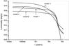Fig. 3 The bolometric luminosity evolution for models 1, 3, 4, and 6.

4.3. Physical properties of the disk

As mentioned previously, the radiation pressure inflates the inner region, producing a slim disk. This effect is illustrated in Fig. 4, in which the profile of the aspect ratio H/r for model 4 is shown for three different evolutionary stages. At 9.29 Myr after the beginning of the accretion process, the radiation pressure is responsible for the increase in the scale of height inside a region r < 5 × 10¹² cm. At this moment, the effective temperature at the inner radius attains a value of about 1.8 × 10⁶ K. After 436.5 Myr, the radiation pressure still affects the inner region, since the effective temperature is still  ~10⁶ K. Near the end of the evolution after 1.23 Gyr, when all the disk mass has practically been consumed, effects of the radiation pressure are no longer seen, and the scale of height increases with the distance as expected. The same behaviour is seen for all models having a critical Reynolds number equal to 500. For models with higher values of ℛ (models 5 and 6), this does not happen. Higher Reynolds numbers decrease the radial velocity, increasing the local mass density and decreasing the parameter β. Thus, besides the tidal field of the BH, the disk self-gravitation also contributes to maintaining the hydrostatic equilibrium in the inner region, avoiding a strong inflation in such a zone, as in other models with lower values of ℛ.

Fig. 4 The profile of the aspect ratio H/r for model 4 in three different evolutionary stages: 9.29 Myr, 436.5 Myr, and 1.235 Gyr.

The effective optical depth controls the energy evacuation by radiation along the vertical axis and the local effective temperature. In general, the effective optical depth increases with the distance, reflecting a decreasing gas temperature. A maximum is reached, and then the optical thickness decreases quite rapidly owing to the decrease in the columnar mass density and the gas recombination. This typical behaviour is shown in Fig. 5 for model 4. We can see that, as the disk evolves, it becomes more optically thin in the inner region thanks to a decreasing columnar mass density, which is a consequence of the accretion process. Each curve ends at the distance at which the disk becomes completely neutral. In this model, the ionized region increases from a radius of  ~8 × 10¹⁵ cm up to  ~2 × 10¹⁷ cm in the time interval 9.3–436 Myr and then decreases to  ~6 × 10¹⁶ cm at the end of our calculations, i.e., 1.24 Gyr.

Fig. 5 Effective optical depth profiles for model 4 in three different evolutionary stages: 9.29 Myr, 436.5 Myr, and 1.235 Gyr.

The highest effective temperatures reached in the inner region of different models after  ~9.3 Myr range from 8 to 15 millions K, obtained for models 1 and 6. These two models only differ in the critical value of the Reynolds number and, as explained above, the former has a geometrical thick inner zone while the latter has a thin inner zone. Consequently, the advection cooling is stronger in model 1 than in model 6 and, in spite of having a higher viscous dissipation, its central effective temperature is lower than in model 6. The other models after  ~9.3 Myr have central effective temperatures of about 2 million K, except for model 5, which is our “coolest” disk, since its effective temperature at that moment is only  ~400   000 K. Models 5 and 6 differ only by the initial BH seed mass and have a geometrical thin inner scale of height, as already mentioned, but nevertheless their central effective temperatures differ by a factor of four. The main reason for such a difference is found in their mass profiles. The viscous dissipation is proportional to the columnar mass density (see Eq. (20)) and, at t ~ 9.3 Myr, Σ in model 6 is about two orders of magnitude higher than in model 5, since the higher seed mass of model 5 consumes the gas in the inner parts of the disk faster than in model 6.

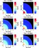Fig. 6 Effective temperature maps for models 5 (left panel) and model 6 (right panel) in three different evolutionary stages: 9.29 Myr, 436.5 Myr, and 1.235 Gyr.

Effective temperature maps for models 5 and 6 are shown in Fig. 6, showing the higher values at the inner disk reached in model 6 for the reason already mentioned. However, the temperatures in the neutral zone are quite similar in both models: T ~ 100 K after 9.29 Myr, T ~ 500 K after 436.5 Myr, and T ~ 670 K after 1.235 Gyr. The temperature in the neutral zones of disk models with primordial chemical composition results from the balance between viscous dissipation and radiation by molecular hydrogen excited by collisions with H atoms.

The evolution of the columnar mass density profile depends on the inward and outward mass fluxes. The former is controlled mainly by the critical Reynolds number and by the mass of the seed, while the latter depends mainly on the redistribution of the angular momentum throughout the disk. In other words, the columnar mass density decreases in the inner regions as the seed grows, and in the outer regions, the columnar mass density decreases because the disk expands. Consequently, at the end of its evolution, the remaining mass of the disk is concentrated in a “torus-like” structure rotating around the central BH . This behaviour is shown in Fig. 7, where the evolution of the columnar mass density profile for model 3 is presented. After  ~1.2 Gyr, the “torus-like” structure having a diameter of the order of 2 pc is clearly seen. The gas temperature in this region is about 2000 K, and it rotates with a Keplerian velocity of about 2640 km s^-1, controlled by the central BH mass. It worth mentioning that in NGC 1068 the central BH is surrounded by a torus-like structure with a diameter of 3.4 pc, detected by the dust infrared emission (Jaffe et al. 2004). The torus-like structure is an important element of the so-called “unified model” of AGNs and quasars, since it determines the visibility (or not) of the “broad line region” according to the direction of the line of sight. It is remarkable that our model is able to offer a natural explanation for the formation of such a “torus-like” structure as a simple consequence of the disk evolution.

Fig. 7 The evolution of the columnar mass density profile. Time in the different snapshots corresponds to the same order as in previous figures. Notice the torus-like structure in the last panel, at the end of the disk evolution.

5. Conclusions

The present work report the results of numerical solutions of the hydrodynamical equations describing non-stationary accretion disks. These simulations aim to investigate the fraction of the disk mass transferred to the central BH and to obtain the timescales of such a process. Turbulence generated by gravitational instability is supposed to be the source of viscosity responsible for the angular momentum transport throughout the disk. The flow, self-regulated by such a mechanism, is characterized by a critical Reynolds number with values in the range 500–1500. The other parameters affecting the accretion process are the initial masses of the seed and of the disk itself.

Observations of bright quasars at z ~ 6 associated to SMBH with masses  ≃10⁹ M_⊙ imply that their growth by accretion processes must occur on timescales below 900 Myr. The present investigation suggests that our models are able to feed seeds with masses in the range 100−1500 M_⊙ on the required timescale. Our numerical simulations indicate that seeds capture about a half of the original disk mass, if the gas consumption by star formation is neglected. This conclusion weakly depend on the adopted model parameters such as the initial masses of the BH and of the disk or the critical Reynolds number. However, the growth timescale, the accretion rate and the resulting disk luminosity do depend on the adopted value of those parameters. Thus, to obtain a quasar at z ~ 6 radiating with a power of  ~4 × 10⁴⁷ erg/s, a disk of a few 10⁹ M_⊙ is necessary, and the accretion process should begin around z ~ 8. However, it should be emphasized that the star formation process is likely to be very efficient in such massive disks, which may reduce the amount of gas available to feed the black hole considerably. Shlosman & Begelman (1989) conclude from their investigation that even a low efficiency in the gas conversion process into stars would deplete the disk on a relatively short time-scale.

Although the formation of several circumnuclear disks during the history of a galaxy cannot be excluded, it is likely that the growth of seeds is a consequence of a unique episode. In this case, one should expect that SMBHs grow faster than their host halos. Observations suggest that the growth of BHs is linked to the evolution of galaxies but not necessarily linked to the growth of their halos. Such an “anti-hierarchical” growth is suggested by the co-moving number density of low X-ray luminosity AGNs peak at z ≤ 1, while that of high X-ray luminosity AGNs peaks at z ~ 2 (Ueda et al. 2003; Hasinger et al. 2005). Since one should expect that the X-ray luminosity is directly related to the accretion rate, hence, to the BH growth, these observations suggest an early assembly of the more massive objects. Such an interpretation is consistent with our simulations, since models with higher seed masses have higher accretion rates and higher luminosities. Our computations also show that the conversion efficiency of gravitational energy into radiation, measured by the ratio L/Ṁc², does not remain constant during the evolution of the disk, varying within the range 10^-1−10^-3.

Detection of polarization in the broad emission lines of NGC 1068 has provided a major argument in favour of the unified AGN model (Antonucci 1993). According to this unified scenario, AGNs have a central core often displaying jets, a inner broad line region (BLR), a narrow line region (NLR), and a circumnuclear torus composed of dust and gas. Observation or not of the BLR depends on the inclination angle of the line of sight with respect to the plane of the torus. Recent observations (Jaffe et al. 2004) indicate that the torus is quite compact (few parsecs sized) and probably has a “clumpy” structure. Its origin is still under debate (see, for instance, Elitzur & Shlosman 2006), but such a structure appears quite naturally in our models as a consequence of the disk evolution. The torus-like structure results from the matter consumption in the inner regions by the central BH and matter “lost” in the outer regions as a consequence of the disk expansion by transfer of angular momentum. In the transition zone, where the radial velocity passes from negative to positive values, the disk material remains stagnant and forms the structure. The dimensions of the resulting torus for model 3, are quite compatible with the parsec-sized torus observed in NGC 1068 (Jaffe et al. 2004). Moreover, the Toomre’s parameter in the torus satisfies the condition Q ≤ 1, indicating that the gas is gravitationally unstable, which could be an explanation for its clumpy structure, supporting our formation scenario.

Our simulations indicate that a substantial fraction of the disk remains neutral with the gas temperature in the interval 100–2000 K most of the time. This late evolution of the outer regions of accretion disk could be related, for instance, to the molecular “ring” of 2 pc radius observed around Sgr A ^∗  (Gusten et al. 1987). Moreover, the physical conditions prevailing in the outskirts of the disk are favourable to star formation and could be an explanation for the presence of massive early-type stars in two rotating thin disks around the BH situated in our own galaxy (Genzel et al. 2003; Paumard et al. 2006). These stars have an estimated age of 6–8 Myr, and both the total mass in the form of stars and gas in these disks are about 2 × 10⁴ M_⊙. It is interesting to notice that, according to our simulations, a disk of initial mass of about 6 × 10⁶ M_⊙ is necessary in order to produce a SMBH of mass of about 3 × 10⁶ M_⊙, like the one located in the Milky Way’s centre. At the end of its evolution, it would remain a mass of a few 10⁴ M_⊙, consistent with observations. This scenario will be investigated in more detail in a future paper that report simulations, including the possibility of gas conversion into stars.

Acknowledgments

M.M.A. acknowledges the Comisión Nacional de Investigación Científica y Tecnológica (CONICYT) de Chile for the fellowship that permitted his stay at the Observatoire de la Côte d’Azur.

References

All Tables

All Figures

	Fig. 1 Evolution of the black hole masses. Labels indicate the considered models, whose parameters are given in Table 1.
In the text

	Fig. 2 Accretion rate evolution for models 1, 2, 4, and 6.
In the text

	Fig. 3 The bolometric luminosity evolution for models 1, 3, 4, and 6.
In the text

	Fig. 4 The profile of the aspect ratio H/r for model 4 in three different evolutionary stages: 9.29 Myr, 436.5 Myr, and 1.235 Gyr.
In the text

	Fig. 5 Effective optical depth profiles for model 4 in three different evolutionary stages: 9.29 Myr, 436.5 Myr, and 1.235 Gyr.
In the text

	Fig. 6 Effective temperature maps for models 5 (left panel) and model 6 (right panel) in three different evolutionary stages: 9.29 Myr, 436.5 Myr, and 1.235 Gyr.
In the text

	Fig. 7 The evolution of the columnar mass density profile. Time in the different snapshots corresponds to the same order as in previous figures. Notice the torus-like structure in the last panel, at the end of the disk evolution.
In the text

References

- Abel, T., Bryan, G. L., & Norman, M. L. 2000, ApJ, 540, 39 [NASA ADS] [CrossRef] [Google Scholar]
- Abramowicz, M. A., Lasota, J.-P., & Xu, C. 1986, in Quasars, ed. G. Swarup, & V. K. Kapahi (Dordrecht: Reidel), IAU Symp., 119, 371 [Google Scholar]
- Abramowicz, M. A., Chen, X., Kato, S., Lasota, J.-P., & Regev, O. 1995, ApJ, 438, L37 [NASA ADS] [CrossRef] [Google Scholar]
- Antonucci, R. R. J. 1993, ARA&A, 31, 473 [Google Scholar]
- Barnes, J. E. 2002, MNRAS, 333, 481 [NASA ADS] [CrossRef] [Google Scholar]
- Begelman, M. C. 1978, MNRAS, 184, 53 [NASA ADS] [CrossRef] [Google Scholar]
- Begelman, M. C., & Shlosman, I. 2009, ApJ, 702, L5 [NASA ADS] [CrossRef] [Google Scholar]
- Bondi, H., & Hoyle, F. 1944, MNRAS, 104, 273 [NASA ADS] [CrossRef] [Google Scholar]
- Bromm, V., Coppi, P. S., & Larson, R. B. 1999, ApJ, 527, L5 [NASA ADS] [CrossRef] [PubMed] [Google Scholar]
- de Freitas Pacheco, J. A. 1969, A&A, 3, 368 [NASA ADS] [Google Scholar]
- de Freitas Pacheco, J. A., & Steiner, J. E. 1976, Ap&SS, 39, 487 [Google Scholar]
- de Freitas Pacheco, J. A., Steiner, J. E., & Damineli Neto, A. 1977, A&A, 55, 111 [NASA ADS] [Google Scholar]
- DiMatteo, T., Croft, R. A. C., Springel, V., & Hernquist, L. 2003, ApJ, 593, 56 [NASA ADS] [CrossRef] [Google Scholar]
- Duschel, W. J., & Britsch, M. 2006, ApJ, 653, L92 [Google Scholar]
- Duschel, W. J., Strittmatter, P. A., & Biermann, P. L. 1998, BAAS, 30, 917 [NASA ADS] [Google Scholar]
- Eisenstein, D. J., & Loeb, A. 1995, ApJ, 443, 11 [NASA ADS] [CrossRef] [Google Scholar]
- Elitzur, M., & Shlosman, I. 2006, ApJ, 648, L101 [NASA ADS] [CrossRef] [Google Scholar]
- Fan, X., et al. 2001, AJ, 122, 2833 [NASA ADS] [CrossRef] [Google Scholar]
- Filloux, C., Durier, F., de Freitas Pacheco, J. A., & Silk, J. 2010, Int. J. Mod. Phys., 19, 1233 [Google Scholar]
- Galli, D., & Palla, F. 1998, A&A, 335, 403 [NASA ADS] [Google Scholar]
- Gao, L., Yoshida, N., Abel, T., et al. 2007, MNRAS, 378, 449 [NASA ADS] [CrossRef] [Google Scholar]
- Genzel, R., Schodel, R., Ott, T., et al. 2003, ApJ, 594, 813 [NASA ADS] [Google Scholar]
- Gusten, R., Genzel, R., Wright, M. C. H., et al. 1987, ApJ, 318, 124 [NASA ADS] [CrossRef] [Google Scholar]
- Haehnelt, M. G., & Rees, M. J. 1993, MNRAS, 263, 168 [NASA ADS] [CrossRef] [Google Scholar]
- Hasinger, G., Miyaji, T., & Schmidt, M. 2005, A&A, 441, 417 [NASA ADS] [CrossRef] [EDP Sciences] [Google Scholar]
- Heger, A., Fryer, C. L., Woosley, S. E., Langer, N., & Hartmann, D. H. 2003, ApJ, 591, 288 [NASA ADS] [CrossRef] [Google Scholar]
- Heinzeller, D., & Duschl, W. J. 2007, MNRAS, 374, 1146 [NASA ADS] [CrossRef] [Google Scholar]
- Hopkins, P. F., Richards, G. T., & Hernquist, L. 2007, ApJ, 654, 731 [NASA ADS] [CrossRef] [Google Scholar]
- Hoyle, F., & Lyttleton, R. A. 1939, Proc. Cambridge Phil. Soc., 35, 405 [NASA ADS] [CrossRef] [Google Scholar]
- Jaffe, W., et al. 2004, Nature, 429, 47 [NASA ADS] [CrossRef] [PubMed] [Google Scholar]
- Koushiappas, S. M., Bullock, J. S., & Dekel, A. 2004, MNRAS, 354, 292 [NASA ADS] [CrossRef] [Google Scholar]
- Levine, R., Gnedin, N. Y., Hamilton, A. J. S., & Kravtsov, A. V. 2008, ApJ, 678, 154 [NASA ADS] [CrossRef] [Google Scholar]
- Levin, Y., Pakter, R., & Rizzato, F. B. 2008, Phys. Rev. E, 78, 021130 [NASA ADS] [CrossRef] [Google Scholar]
- Masset, F. 2000, A&AS, 141, 165 [NASA ADS] [CrossRef] [EDP Sciences] [Google Scholar]
- Marconi, A., Risaliti, G., Gilli, R., et al. 2004, MNRAS, 351, 169 [NASA ADS] [CrossRef] [Google Scholar]
- Mihos, C., & Hernquist, L. 1996, ApJ, 464, 641 [NASA ADS] [CrossRef] [Google Scholar]
- Milosavljevic, M., Bromm, V., Couch, S. M., & Oh, S. P. 2009, ApJ, 698, 766 [NASA ADS] [CrossRef] [Google Scholar]
- Oshuga, K., Mineshige, S., Mori, M., & Umemura, M. 2002, ApJ, 574, 315 [NASA ADS] [CrossRef] [Google Scholar]
- Paczynski, B. 1978, Act. Astr., 28, 91 [Google Scholar]
- Paczyński, B., & Wiita, P. J. 1980, A&A, 88, 23 [NASA ADS] [Google Scholar]
- Paumard, T., Genzel, R., Martins, F., et al. 2006, J. Phys. Conf. Ser., 54, 199 [NASA ADS] [CrossRef] [Google Scholar]
- Peirani, S., & de Freitas Pacheco, J. A. 2008, Phys. Rev. D, 77, 064023 [NASA ADS] [CrossRef] [Google Scholar]
- Pelupessy, F. I., DiMatteo, T., & Ciardi, B. 2007, ApJ, 665, 107 [NASA ADS] [CrossRef] [Google Scholar]
- Power, C., Nayakshin, S., & King, A. 2011, MNRAS, in press [arXiv:1003.0605] [Google Scholar]
- Regan, J. A., & Haehnelt, M. G. 2009, MNRAS, 396, 343 [NASA ADS] [CrossRef] [Google Scholar]
- Richard, D., & Zahn, J.-P. 1999, A&A, 347, 734 [NASA ADS] [Google Scholar]
- Richtmyer, R. D., & Morton, R. W., 1957, Difference Methods for Initial Value Problems, 2nd edition (New York: Wiley Interscience) [Google Scholar]
- Shakura, N. I., & Sunyaev, R. A. 1973, A&A, 24, 337 [NASA ADS] [Google Scholar]
- Shapiro, S. L. 2004, ApJ, 613, 1213 [NASA ADS] [CrossRef] [Google Scholar]
- Shlosman, I., & Begelman, M. C. 1989, ApJ, 341, 685 [NASA ADS] [CrossRef] [Google Scholar]
- Small, T. A., & Blandford, R. D. 1992, MNRAS, 259, 725 [NASA ADS] [Google Scholar]
- Soltan, A. 1982, MNRAS, 200, 115 [NASA ADS] [CrossRef] [Google Scholar]
- Springel, V., DiMatteo, T., & Hernquist, L. 2005, MNRAS, 361, 776 [NASA ADS] [CrossRef] [Google Scholar]
- Stone, J. M., & Norman, M. L. 1992, ApJS, 80, 753 [Google Scholar]
- Piran, T. 1978, ApJ, 221, 652 [NASA ADS] [CrossRef] [Google Scholar]
- Yoshida, N., Omukai, K., Hernquist, L., & Abel, T. 2006, ApJ, 652, 6 [NASA ADS] [CrossRef] [Google Scholar]
- Van Leer, B. 1977, Comput. Phys., 23, 276 [NASA ADS] [CrossRef] [Google Scholar]
- Ueda, Y., Akiyama, M., Ohta, K., & Miyaji, T. 2003, ApJ, 598, 886 [NASA ADS] [CrossRef] [Google Scholar]
- Willot, C. J., McLure, R. J., & Jarvis, M. J. 2003, ApJ, 587, L15 [NASA ADS] [CrossRef] [Google Scholar]
- Wise, J. H., Turk, M. J., & Abel, T. 2008, ApJ, 682, 745 [NASA ADS] [CrossRef] [Google Scholar]