| Issue |
A&A
Volume 526, February 2011
|
|
|---|---|---|
| Article Number | A13 | |
| Number of page(s) | 6 | |
| Section | Cosmology (including clusters of galaxies) | |
| DOI | https://doi.org/10.1051/0004-6361/200913649 | |
| Published online | 14 December 2010 | |
Black holes and galactic density cusps
From black hole to bulge
1
Instituto de Física Teórica UAM/CSIC, Facultad de Ciencias, C-XI,
Universidad Autónoma de Madrid Cantoblanco,
28049
Madrid,
Spain
e-mail: This email address is being protected from spambots. You need JavaScript enabled to view it.
2
Queen’s University, Kingston, Ontario, Canada
e-mail: This email address is being protected from spambots. You need JavaScript enabled to view it.
3
Faculty of Science, University of Ontario Institute of Technology,
Oshawa, L1H 7K4
Ontario,
Canada
e-mail: This email address is being protected from spambots. You need JavaScript enabled to view it.
Received:
11
November
2009
Accepted:
26
October
2010
Abstract
Aims. In this paper we continue our study of density cusps that may contain central black holes.
Methods. Our previous thus attempts to use distribution functions with a memory of self-similar relaxation apply mainly in restricted regions of the global system. We are forced to consider related distribution functions that are steady but not self-similar.
Results. One remarkably simple distribution function that has a filled loss cone describes a bulge that transits from a near black hole domain to an outer “zero flux” regime where ρ ∝ r−7/4. The transition passes from an initial inverse square profile through a region having a 1/r density profile. The structure is likely to be developed at an early stage in the growth of a galaxy. A central black hole is shown to grow exponentially in this background with an e-folding time of a few million years.
Conclusions. We derive our results from first principles, using only the angular momentum integral in spherical symmetry. The initial relaxation probably requires bar instabilities and clump-clump interactions.
Key words: cosmology: theory / dark matter / galaxies: halos / galaxies: nuclei / black hole physics / gravitation
© ESO, 2010
1. Introduction
We discussed the relation between the formation of black holes (hereafter BH) and of galactic bulges, or of bulges with a central mass in the previous papers of this series of papers (Le Delliou et al., referred to here as Papers I, II, and references hereafter).
Previous research (Kormendy & Richstone 1995; Magorrian et al. 1998) and more recently (Ferrase & Merritt 2000; Gebhardt et al. 2000) has established a strong correlation between the BH mass and the surrounding stellar bulge mass (or velocity dispersion), which we take as an indication of coeval growth. Such growth may occur as BH “seeds” accrete gas or disrupted stars in a dissipative fashion during the AGN (active galactic nuclei) phase, but there is as yet no generally accepted scenario. Moreover, the necessity for a seed and observations of early very supermassive BHs (e.g. Kurk et al. 2007), together with changes in the normalization of the BH mass-bulge mass proportionality (e.g. Maiolino et al. 2007); suggest an alternate growth mechanism. In fact some authors (Peirani & de Freitas Pacheo 2008) have studied the possible size of the dark matter component in BH masses and deduce that between 1% and 10% of the black hole mass could be due to dark matter.
We explored coeval growth in the case of spherically symmetric radial and non-radial infall (Papers I, II), using distribution functions with a self-similar memory. However although we obtained reasonable descriptions in sections, we did not find a distribution function (hereafter DF) that could be fit to Black Hole halo and bulge continuously. Moreover the problem of the black hole feeding was left unresolved. This requires an anisotropic DF with a filled loss cone of the nature of the Bahcall & Wolf solution (Bahcall & Wolf 1976).
Here we repair these omissions for a special case of non self-similar infall. We use the same technique of inferring reasonable distribution functions for collisionless matter from the time dependent collisionless Boltzmann (CBE) and Poisson set, while insisting on a central point mass. The temporal evolution allows for relaxation of collisionless matter in addition to possible “clump-clump” (two clump) interactions.
We use, in this paper as in the previous (I, II), the Carter-Henriksen (Carter & Henriksen 1991) procedure. In this way we obtain a quasi-self-similar system of coordinates (Henriksen 2006a,b) that enables expression of the CBE-Poisson set with explicit reference to a previous transient self-similar dynamical relaxation. Thus we can remain “close” to self-similarity just as the simulations appear to do.
We begin the next section with a summary of this approach in spherical symmetry that is common to all papers in this series, including the useful results found earlier (Papers I, II). Subsequently we recall the limiting case with a high binding energy cut off in the DF. This is to remind us that such a cut-off, existing for any reason, produces a flat cusp. Finally we give the key result of this paper as a non-self-similar DF (of a type found previously (Evans & An 2006) but not used in this connection) that describes the transition zone. This zone extends from a central mass through a shallow region (to be compared with observations of the milky way) into a Bahcall & Wolf feeding region. Ultimately it enters an inverse square law region.
2. Dynamical equations and radial results
Following the formulation of Henriksen (2006b) we
transform to infall variables the collisionless Boltzmann and Poisson equations for a
spherically symmetric anisotropic system in the “Fujiwara” form (e.g. Fujiwara 1983) namely
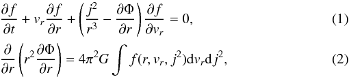 where
f is the phase-space mass density, Φ is the “mean” field gravitational
potential, j2 is the square of the specific angular momentum and
other notation is more or less standard.
where
f is the phase-space mass density, Φ is the “mean” field gravitational
potential, j2 is the square of the specific angular momentum and
other notation is more or less standard.
The transformation to infall variables has the form (e.g. Henriksen 2006b)
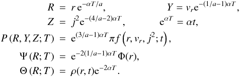 (3)The
passage to the self-similar limit requires taking
∂T = 0 when acting on the transformed
variables. Thus the self-similar limit is a stationary system in these variables, which is a
state that we refer to as “self-similar virialisation” (Henriksen & Widrow 1999; Le Delliou
2001). The virial ratio 2K/ |W| is a
constant in this state (although greater than one; K is kinetic energy and
W is potential), but the system is not steady in physical variables as
infall continues.
(3)The
passage to the self-similar limit requires taking
∂T = 0 when acting on the transformed
variables. Thus the self-similar limit is a stationary system in these variables, which is a
state that we refer to as “self-similar virialisation” (Henriksen & Widrow 1999; Le Delliou
2001). The virial ratio 2K/ |W| is a
constant in this state (although greater than one; K is kinetic energy and
W is potential), but the system is not steady in physical variables as
infall continues.
The single quantity a is the constant that determines the dynamical similarity, called the self-similar index. It is composed of two separate reciprocal scalings, α in time and δ in space, in the form a ≡ α/δ. As it varies it contains all dominant physical constants of mass, length and time dimensions, since the mass scaling μ has been reduced to 3δ − 2α in order to maintain Newton’s constant G invariant (e.g. Henriksen 2006b).
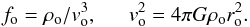
We assume that time, radius, velocity and density are measured in fiducial units
ro/vo,ro,
vo and ρo respectively. The unit
of the DF is fo and that of the potential is
 . We remove constants
from the transformed equations by taking
. We remove constants
from the transformed equations by taking
 (4)These
transformations convert Eqs. (1), (2) to the respective forms
(4)These
transformations convert Eqs. (1), (2) to the respective forms
 (5)and
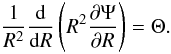 (6)This integro-differential
system is closed by
(6)This integro-differential
system is closed by
 (7)This completes the
formalism that we will use to obtain our results.
(7)This completes the
formalism that we will use to obtain our results.
For easy reference in this paper, we summarize the general forms of the self-similar DFs that we discussed previously.
In Paper I we discussed the emergence in purely radial infall of the rigorously steady DFs
from Henriksen & Widrow (hereafter HWDF, Henriksen & Widrow 1995)
 (8)and the time-dependent DF
from Fridmann and Polyachenko (hereafter FPDF, Fridmann
& Polyachenko 1984)
(8)and the time-dependent DF
from Fridmann and Polyachenko (hereafter FPDF, Fridmann
& Polyachenko 1984)
 (9)Introducing anisotropies
in Paper II, we found the general self-similar solution to Eq. (5) to be
(9)Introducing anisotropies
in Paper II, we found the general self-similar solution to Eq. (5) to be  (10)where
  This
yields the physical form of the general steady state with self-similar memory to be
This
yields the physical form of the general steady state with self-similar memory to be
 (13)where
 . Taking first
 to
be constant, and then taking it to be proportional to
κ − q. this yields respectively
to
be constant, and then taking it to be proportional to
κ − q. this yields respectively
 where
we have defined w = (3 − a)/(4−2a).
These limits were found to apply to inner and outer extremes of the relaxed region of a
simulated “bulge” (i.e. no black hole was included in the simulations).
where
we have defined w = (3 − a)/(4−2a).
These limits were found to apply to inner and outer extremes of the relaxed region of a
simulated “bulge” (i.e. no black hole was included in the simulations).
The DF (13) can be put in a form that seems
to generalize the FPDF (Eq. (9)). We choose
 to obtain
  (16)The density and potential
laws are more general than those of the FPDF, being respectively
ρ ∝ r−2a and
Φ ∝ r2(1−a).
(16)The density and potential
laws are more general than those of the FPDF, being respectively
ρ ∝ r−2a and
Φ ∝ r2(1−a).
None of these DFs can be said to apply to every region of the simulated halos.
3. High binding energy cut-off
We recall in this section an extreme case that limits the flattening of the cusp near a
black hole. There is evidence (Le Delliou 2001; MacMillan et al. 2006) for a cut-off in the number of
particles with high binding energy, even without a central point mass. The presence of a
central black hole of mass M• is likely to accentuate this trend
by accretion. We may imitate such a cut-off in order to study limiting behaviour near the
black hole, by using the isothermal DF (see e.g. Papers I and II) at negative energies and
temperatures in the form  (17)Here
 . We
suppose that the constant β > 0 and corresponds to some reciprocal
cut-off energy. A straight-forward calculation of the density implied by such a DF yields
(note that we integrate only over negative energies rather than over all velocities)
. We
suppose that the constant β > 0 and corresponds to some reciprocal
cut-off energy. A straight-forward calculation of the density implied by such a DF yields
(note that we integrate only over negative energies rather than over all velocities)
 (18)where
M(a,b,z) is the Kummer function. We expect this to hold
where |Φ| ≈ GM•/r is
large, and in this limit the Kummer function varies as −3/(2z).
Consequently the density cusp becomes as flat as
(18)where
M(a,b,z) is the Kummer function. We expect this to hold
where |Φ| ≈ GM•/r is
large, and in this limit the Kummer function varies as −3/(2z).
Consequently the density cusp becomes as flat as  . This was
already noticed in Nakano & Makino (1999) and
in Merritt & Szell (2006), where in both
cases it is due to scouring by merging black holes. In any case, as was recognized in Nakano & Makino (1999), only the cut-off is
required.
. This was
already noticed in Nakano & Makino (1999) and
in Merritt & Szell (2006), where in both
cases it is due to scouring by merging black holes. In any case, as was recognized in Nakano & Makino (1999), only the cut-off is
required.
A cut-off in the number of particles per unit energy
dM/dE is to be expected on general grounds. The density
of states (Binney & Tremaine 1987) for an
isotropic DF in a region dominated by a point mass potential is
 , from
which the differential energy distribution
dM/dE = g(E)f(E)
may be calculated. Thus even a constant f(E) (for which
ρ ∝ |Φ| 3/2 and therefore goes like
r-1.5 near a point mass) will show a cutoff in the mass
distribution as the density of states decreases in the expanding phase space. However the
evidence suggests that f(E) is also declining with
increasing |E| in the most tightly bound central regions.
, from
which the differential energy distribution
dM/dE = g(E)f(E)
may be calculated. Thus even a constant f(E) (for which
ρ ∝ |Φ| 3/2 and therefore goes like
r-1.5 near a point mass) will show a cutoff in the mass
distribution as the density of states decreases in the expanding phase space. However the
evidence suggests that f(E) is also declining with
increasing |E| in the most tightly bound central regions.
Assuming the DF (14) and a = 0.5), we predict the mass distribution function dM/dE ∝ |E|-5. Thus a cut-off in the isotropic DF can be associated with the r−2a = r-1 density profile. The mechanism for the high binding energy cut-off is not immediately evident, but it must be part of the dynamical relaxation. High negative energy particles must be preferentially excited to less negative energies, which does not seem to occur in strict shell code simulations (Henriksen & Widrow 1999). However it may occur due to the presence of sub-structure such as clumps or bar formation by the radial orbit instability (MacMillan et al. 2006). In any case it may not require black hole “scouring”, although this process does have the maximum effect (Merritt & Szell 2006; Nakano & Makino 1999).
4. Global solution with black hole and a Bahcall/Wolf outer cusp
We consider an exact collisionless cusp that has an embedded central mass. It is necessarily not self-similar. We have seen that we expect a DF that is primarily dependent on angular momentum in the outer regions of a bulge (e.g. (15) before the maximum in angular momentum). We can not follow analytically the development of this region in time, as this is the province of numerical work. We can however hope to find analytic descriptions of ultimate states.
There is one steady solution that is not self-similar but which is closely related to the
Evans and An (Evans & An 2006) solution with
anisotropy parameter β = 0.5. This is an exact solution to Eq. (5) with
∂T ≠ 0 (compare Eqs. (10), (15)) in the form (recall that
w ≡ (3 − a)/(4−2a))
 that
is, written entirely in transformed coordinates,
that
is, written entirely in transformed coordinates,
 (19)This solution is
always steady but not always self-similar because of the T dependence. This
equation is seen to satisfy Eq. (5) by direct
substitution when the dependence on T is included. The steady form (10) that we found in the previous paper of this
series is distinguished from the general steady class by being a possible limit of
self-similar evolution. The same problem has been addressed with arbitrary steady and
isotropic distribution functions in an interesting paper by Baes et al. (2005).
(19)This solution is
always steady but not always self-similar because of the T dependence. This
equation is seen to satisfy Eq. (5) by direct
substitution when the dependence on T is included. The steady form (10) that we found in the previous paper of this
series is distinguished from the general steady class by being a possible limit of
self-similar evolution. The same problem has been addressed with arbitrary steady and
isotropic distribution functions in an interesting paper by Baes et al. (2005).
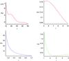 |
Fig. 1 We show the various density regimes of the zeroflux cusp with an embedded black hole.
The constants in Eq. (24) have been
chosen for numerical convenience and positive definiteness to be:
|Φ| ∞ = 3, C1 = 5 and
C2 = −2/(πK′).
Here K′ ≡ K/(8π) = 10 so that
C2 ≡ −M• = −1/5π.
In addition the plot is of |

A convenient choice is to take
 , where
ν is any suitable real number. Then the DF is simply
, where
ν is any suitable real number. Then the DF is simply
 (20)The density
associated with such a distribution is (E < 0,
ν − w > −1)
(20)The density
associated with such a distribution is (E < 0,
ν − w > −1)  (21)This may now be substituted
into the Poisson equation to give an equation for |Φ| and hence the density in a
self-consistent bulge.
(21)This may now be substituted
into the Poisson equation to give an equation for |Φ| and hence the density in a
self-consistent bulge.
There is a power law solution ∝ rh provided
that h > −1. In terms of w and
ν, h is
 (22)and the logarithmic
density slope is h − 2. Most of the density power laws
(h − 2) of interest arise for values of
ν − w near −1.
(22)and the logarithmic
density slope is h − 2. Most of the density power laws
(h − 2) of interest arise for values of
ν − w near −1.
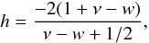
For example ν − w = −0.9 yields h − 2 = −1.5, while ν − w = −5/6 yields h − 2 = −1.0. The limiting case with ν − w = −1 (which has a logarithmic singularity at zero angular momentum) gives as expected h − 2 = −2. Setting ν = 0 returns us to the self-similar bulge (15) and indeed h − 2 = −2a in this case.
It is clear however that there is a special case when
ν − w + 1/2 = 0, for which the DF is
 .
This value treated separately yields
.
This value treated separately yields  (23)The Poisson equation is
therefore linear and it is readily solved to find
(23)The Poisson equation is
therefore linear and it is readily solved to find 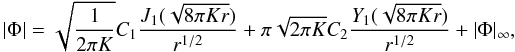 (24)where
J1 and Y1 are first order Bessel
functions of the first and second kinds respectively. The density is given by Eq. (23).
(24)where
J1 and Y1 are first order Bessel
functions of the first and second kinds respectively. The density is given by Eq. (23).
The constants in Eq. (24) must be such as to maintain |Φ| and ρ positive despite the oscillations in the Bessel functions. This may impose a limited range in radius, which is in any case required to ensure a finite mass. In general the Bessel functions will be out of phase by π/2 and it is not possibile to keep their sum positive everywhere. However it is possible to keep the whole expression positive by choosing an appropriate set of constants as we have done in our example. Because the term containing the Bessel functions is declining as r−7/4, once a critical transition region is traversed successfully by a choice of constants the positivity is assured henceforward. It is really only the difference of the potential moduli that is physical and this difference is free to oscillate as indicated. It is interesting nevertheless that |Φ|∞ is necessarily non-zero, as this suggests that the solution must be embedded in distant matter.
As z → 0 one has
J1(z) ≈ z/2 while
Y1(z) ≈ −2/(πz). Hence
the potential contains a central point mass in this limit if
C2 = −M•. The term in
J1 tends to a constant and is presumably associated with the
bulge mass itself. Consequently by Eq. (23)
the density cusp near the central black hole has the profile ![Mathematical equation: \begin{equation} \rho=2\pi K\left[\frac{C_{1}+|\Phi|_{\infty}}{r}+\frac{GM_{\bullet}}{r^{2}}\right]\cdot\label{eq:CuspR1} \end{equation}](/articles/aa/full_html/2011/02/aa13649-09/aa13649-09-eq113.png) (25)The constant
C1 gives the difference in the modulus of the bulge potential,
coming from infinity to a radius where J1 is well approximated
by the small argument limit (it depends on K). This happens before the
small argument limit applies to Y1. We see in general from this
solution that the near black hole cusp can start with a (−1) logarithmic density slope and
steepen to (−2) near the black hole. This appears to encompass the observations.
(25)The constant
C1 gives the difference in the modulus of the bulge potential,
coming from infinity to a radius where J1 is well approximated
by the small argument limit (it depends on K). This happens before the
small argument limit applies to Y1. We see in general from this
solution that the near black hole cusp can start with a (−1) logarithmic density slope and
steepen to (−2) near the black hole. This appears to encompass the observations.
A remarkable behaviour of this solution occurs at large r (actually large
 ),
where
),
where
 and
and
 . This shows that the
mean density tends to the r−7/4 density profile that is
characteristic of the Bahcall & Wolf (Bahcall
& Wolf 1976) zero flux solution. According to the small r
limits, we find it here outside a flatter region r-1 that gives
way ultimately to an inner r-2 region. Outside of the
Bahcall/Wolf r−7/4 region one would return to a
r-1 profile (recalling that the potential there, i.e. at
“infinity” is not zero). This appears to connect a black hole through intermediate cusps to
the inner NFW profile. Our figures are illustrative however and the constants of our formula
would have to be chosen for the best fit consistent with positivity in any particular case.
. This shows that the
mean density tends to the r−7/4 density profile that is
characteristic of the Bahcall & Wolf (Bahcall
& Wolf 1976) zero flux solution. According to the small r
limits, we find it here outside a flatter region r-1 that gives
way ultimately to an inner r-2 region. Outside of the
Bahcall/Wolf r−7/4 region one would return to a
r-1 profile (recalling that the potential there, i.e. at
“infinity” is not zero). This appears to connect a black hole through intermediate cusps to
the inner NFW profile. Our figures are illustrative however and the constants of our formula
would have to be chosen for the best fit consistent with positivity in any particular case.
Figure 1 indicates these various regimes when the
constants are chosen such that the bulge mass is about fifteen (actually
5π, we represent the bulge mass by
 ) times that of the
central black hole. Starting from upper left the curves move inwards in a clockwise
direction to show the outer r−7/4 oscillating region, then
the r-1 region, a transition region, and finally the
r-2 region. The curves are connected in a continuous fashion.
) times that of the
central black hole. Starting from upper left the curves move inwards in a clockwise
direction to show the outer r−7/4 oscillating region, then
the r-1 region, a transition region, and finally the
r-2 region. The curves are connected in a continuous fashion.
The final Fig. 2 expands the outer oscillating Bahcall-Wolf region.
Because of the slow decline in the density with radius, it is evident that the outer radial limit to this solution is finite. Exactly where it applies will depend on special numerical cases, but it seems in any case that it must be inside the radius where the density has an inverse square profile, essentially the scale radius of the dark matter simulations.
The physical behaviour all stems from a DF that has the simple form K/ |j| . It appears to describe a zero flux equilibrium condition in the mean, together with a stably filled loss cone (Tremaine 2005). The density oscillations may indicate that collective behaviour is necessary. It is an isolated example of the class of distribution functions studied by Evans & An (2006).
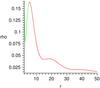 |
Fig. 2 This figure shows the oscillations in the outer zero flux regime. |
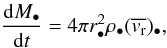 (26)where
r• = 6GM•/c2.
The required mean radial velocity is found to be
(26)where
r• = 6GM•/c2.
The required mean radial velocity is found to be  which is the same for the inward or outward going particles in a steady state. We calculate
 from the expression
 (27)which becomes explicitly on
transforming to an energy variable through
dE = vrdvr
(27)which becomes explicitly on
transforming to an energy variable through
dE = vrdvr (28)This is conveniently
written as
(28)This is conveniently
written as  (29)which yields finally the
quoted result. In effect we have by ignoring
dE = −vrdvr
calculated only the outward mean velocity which we take to be equal to the inward mean
velocity of particles reaching the black hole. We eliminate K in terms of
the bulge quantities using Eq. (23) so that
2πK = rbρb/|Φ| b.
By setting |Φ|• = c2/6, the calculation yields
finally (restoring units)
(29)which yields finally the
quoted result. In effect we have by ignoring
dE = −vrdvr
calculated only the outward mean velocity which we take to be equal to the inward mean
velocity of particles reaching the black hole. We eliminate K in terms of
the bulge quantities using Eq. (23) so that
2πK = rbρb/|Φ| b.
By setting |Φ|• = c2/6, the calculation yields
finally (restoring units)  (30)As an illustration we take
ρb to be the mean density of
109 M⊙ in one kiloparsec (i.e.
rb) and set
(30)As an illustration we take
ρb to be the mean density of
109 M⊙ in one kiloparsec (i.e.
rb) and set  , the circular velocity at
rb. We take this to be 200 km s-1 and obtain
finally
, the circular velocity at
rb. We take this to be 200 km s-1 and obtain
finally  (31)Given the e-folding
time on the right of this last equation, we can increase the mass of the black hole one
hundred fold in three to four million years. On this basis one can expect the presence of
massive black holes very early in the history of the Universe. This has to happen however
before the bulge has become isotropic, presumably in the rapid growth phase of the dark
matter halo. Some seed mass is nevertheless required, which may be primordial.
(31)Given the e-folding
time on the right of this last equation, we can increase the mass of the black hole one
hundred fold in three to four million years. On this basis one can expect the presence of
massive black holes very early in the history of the Universe. This has to happen however
before the bulge has become isotropic, presumably in the rapid growth phase of the dark
matter halo. Some seed mass is nevertheless required, which may be primordial.
Such a multi-power law behaviour does not give the simple linear correlation between bulge mass and black hole mass that we suggested in Papers I and II. However since the black hole is incorporated into the global solution at all times, we do expect such a correlation from the integration of Eq. (23) integrated over r. If most of the inner part of the outer r−7/4 law can be considered to have fallen into the black hole, then M•/Mb ≈ (r•/rb)5/4.
5. Conclusions
We have sought in this series of Papers (I, II, and the present paper) to find distribution functions that describe both dark matter bulges and a central black hole or at least a central mass concentration. In most cases we succeed only in describing the dark matter bulges, but there are some notable exceptions.
In the discussion of cusps and bulges based on purely radial orbits (Paper I), we were able to distinguish the Distribution function of Fridmann & Polyachenko (9) from that of Henriksen & Widrow (8). The FPDF was found to describe accurately the purely radial simulations of isolated collisionless halos carried out in MacMillan (2006). These simulations retained the initial cosmological conditions although non-radial forces were switched off. The final state is close to self-similar virialisation rather than steady virialisation, since the infall continues.
This correspondence between the theory and the simulations gives us some confidence in the DF’s found by remaining “close” to self-similarity. This is especially so since predictions describing the simulation results in Paper II were based on a = 0.72, which was deduced elsewhere in the context of adiabatic self-similarity (Henriksen 2007).
The FPDF can contain consistently a central mass concentration that is unlikely to be a true black hole, at least in the early stages. It may represent a central mass concentration or bulge initially. Subsequently with the rise of dissipation and instabilities, there may be a slower phase of radial accretion towards the centre. It is possible that this cycle could repeat several times in a process we have referred to as “interrupted accretion”. Under this process the r-2 density law would apply almost everywhere. The radial velocity dispersion is proportional to the potential. Thus it decreases as r-1 near the central mass, and subsequently decreases logarithmically with r.
The HWDF (8) is restricted to a strictly steady and self-similar bulge, but it has the merit of allowing a family of densities and potentials (velocity dispersion) according to the self-similar prescription. A central mass is allowed only in the Keplerian limit wherein a = 3/2. This gives a massless bulge with ρ ∝ r-3. This is naturally iterated to give an inner flattening but continued iteration is effectively in powers of lnr, which should therefore yield weak corrections. The iteration can only apply away from r = 0, so that the central mass is a “renormalized” extended mass.
The HWDF was shown in Paper I to give a density that is linear in the potential, and hence a self-consistent bulge is found from the Poisson equation. The density profile is never flatter than r-2.5 near the central mass and tends to r-3 in the near Keplerian limit of dominant central mass. This restricts the applicability to a region outside the central bulge. It does not seem to be relevant to a near black hole domain.
The inclusion of angular momentum led to more realistic situations. We re-derived in Paper II the steady self-similar DFs from first principles in Eq. (13). We showed that these can be used to describe the simulated collisionless halos calculated in MacMillan (2006), if we use the value of a ≈ 0.72 identified in Henriksen (2007) and take two limits. In one (14) the DF is isotropic and describes approximately the central region of the bulge. The other limit (15) describes the outer region. This encourages us regarding the relevance of this family. Unfortunately the potential of a central mass can not be included exactly in these distribution functions.
As always a = 1 must be treated separately and we give a derivation from first principles in this series. In Paper I we show that this case corresponds to a radially growing system with the FPDF. The anisotropic solution is discussed in Paper II The results are new. It implies the density profile ρ ∝ r-2 always.
Generally we find that we can not describe elegantly anisotropic bulges containing black holes with self-similar DFs, as one might expect. The self-similarity is restricted to the surrounding bulge, and this is progressively perturbed near the black hole. We re-emphasized in the current paper in a non self-similar context that a sharp cut-off of any kind (whether due to black hole binary scouring or not) can yield a density profile as flat as −1/2.
Our most successful description of a black hole embedded in an anisotropic bulge is given in this paper by the DF πf = K/(j2)1/2. This simplest member of the family discovered by Evans & An (ibid) yields a bulge containing a central point mass. The density profile near this mass is given by Eq. (25) as r-1 with an inner r-2 peak. Farther out there is an r−7/4 domain in the mean that imitates the Bahcall & Wolf (ibid) cusp, which in turn ultimately becomes the NFW r-1 profile.
The reasons for this behaviour appear to be very different from those of Bahcall and Wolf, since there are no two body collisions in this treatment. By assuming a steady filled loss cone of this simple form, we have selected a zero flux behaviour on the outer boundary as an average behaviour independently of the detailed mechanism that acts to establish this (∂f/∂E = 0). In that sense it is a useful description of the black hole cusp region. The oscillations may indicate the necessity of collective behaviour for maintaining a filled loss cone.
We observe finally that this DF does not require a very strong concentration of low angular momentum particles. In the outer region where Φ ≈ const., we find dN/dj2 ≈ const. so that the particles are mostly at high angular momentum, as one might expect.
Black hole growth is astrophysically rapid in this distribution as seems to be required observationally. Careful study of the density regimes may permit bulge mass and black hole mass to be distinguished and correlated, assuming this distribution is realized.
Acknowledgments
R.N.H. acknowledges the support of an operating grant from the canadian Natural Sciences and Research Council. The work of MLeD is supported by CSIC (Spain) under the contract JAEDoc072, with partial support
from CICYT project FPA2006-05807, at the IFT, Universidad Autonoma de Madrid, Spain.
References
- Baes, M., Dejonge, H., & Buyle, P. 2005, A&A, 432, 411 [NASA ADS] [CrossRef] [EDP Sciences] [Google Scholar]
- Bahcall, J., & Wolf, R. A. 1976, ApJ, 209, 214 [NASA ADS] [CrossRef] [Google Scholar]
- Binney, J., & Tremaine S. 1987, Galactic Dynamics (Princeton, New Jersey: Princeton University Press) [Google Scholar]
- Carter, B., & Henriksen, R. N. 1991, J. Math. Phys., 32, 2580 [NASA ADS] [CrossRef] [Google Scholar]
- Evans, N. W., & An, J. H. 2006, Phys. Rev. D, 73, 023524 [NASA ADS] [CrossRef] [Google Scholar]
- Ferrarese, L., & Merritt, D. 2000, ApJ, 539, L9 [NASA ADS] [CrossRef] [Google Scholar]
- Fridman, A. M., & Polyachenko, V. L. 1984, Physics of Gravitating Systems (New York: Springer) [Google Scholar]
- Fujiwara, T. 1983, PASJ, 35, 547 [NASA ADS] [Google Scholar]
- Gebhardt, K., Bender, R., Bower, G., et al. 2000, ApJ, 539, L13 [NASA ADS] [CrossRef] [Google Scholar]
- Henriksen, R. N. 2006a, MNRAS, 366, 697 [NASA ADS] [CrossRef] [Google Scholar]
- Henriksen, R. N. 2006b, ApJ, 653, 894 [NASA ADS] [CrossRef] [Google Scholar]
- Henriksen, R. N. 2007, ApJ, 671, 1147 [NASA ADS] [CrossRef] [Google Scholar]
- Henriksen, R. N., & Widrow, L. M. 1995, MNRAS, 276, 679 [NASA ADS] [CrossRef] [Google Scholar]
- Henriksen, R. N., & Widrow, L. M. 1999, MNRAS, 302, 321 [NASA ADS] [CrossRef] [Google Scholar]
- Kurk, J. D., Walter, F., Fan, X., et al. 2007, ApJ, 669, 32 [NASA ADS] [CrossRef] [Google Scholar]
- Kormendy, J., & Richstone, D. 1995, ARA&A, 33, 581 [NASA ADS] [CrossRef] [Google Scholar]
- Le Delliou, M., Henriksen, R. N., & MacMillan, J. D. 2010a, MNRAS, submitted [arXiv:0911.2232] (I) [Google Scholar]
- Le Delliou, M., Henriksen, R. N., & MacMillan, J. D. 2010b, A&A, 522, A28 (II) [NASA ADS] [CrossRef] [EDP Sciences] [Google Scholar]
- Le Delliou, M. 2001, Ph.D. Thesis, Queen’s University, Kingston, Canada [Google Scholar]
- MacMillan, J. 2006, Ph.D. Thesis, Queen’s University at Kingston, ONK7L 3N6, Canada [Google Scholar]
- MacMillan, J. D., Widrow, L. M., & Henriksen, R. N. 2006, ApJ, 653, 43 [NASA ADS] [CrossRef] [Google Scholar]
- Magorrian, J., Tremaine, S., Richstone, D., et al. 1998, AJ, 115, 2285 [NASA ADS] [CrossRef] [Google Scholar]
- Maiolino, R., Neri, R., Beelen, A., et al. 2007, A&A, 472, L33 [NASA ADS] [CrossRef] [EDP Sciences] [Google Scholar]
- Merritt, D., & Szell, A. 2006, ApJ, 648, 890 [NASA ADS] [CrossRef] [Google Scholar]
- Mutka, P. 2009, Proceeding of Invisible Universe, Palais de l’UNESCO, Paris, ed. J.-M. Alimi [Google Scholar]
- Peirani, S., & de Freitas Pacheo, J. A. 2008, Phys. Rev. D, 77, 064023 [NASA ADS] [CrossRef] [Google Scholar]
- Nakano, T., & Makino, M. 1999, ApJ, 525, L77 [NASA ADS] [CrossRef] [PubMed] [Google Scholar]
- Navarro, J. F., Frenk, C. S., & White, S. D. M. 1996, ApJ, 462, 5 (NFW) [Google Scholar]
- Tremaine, S. 2005, ApJ, 625, 143 [NASA ADS] [CrossRef] [Google Scholar]
All Figures
|
Fig. 1 We show the various density regimes of the zeroflux cusp with an embedded black hole.
The constants in Eq. (24) have been
chosen for numerical convenience and positive definiteness to be:
|Φ| ∞ = 3, C1 = 5 and
C2 = −2/(πK′).
Here K′ ≡ K/(8π) = 10 so that
C2 ≡ −M• = −1/5π.
In addition the plot is of |
| In the text | |
|
Fig. 2 This figure shows the oscillations in the outer zero flux regime. |
| In the text | |
Current usage metrics show cumulative count of Article Views (full-text article views including HTML views, PDF and ePub downloads, according to the available data) and Abstracts Views on Vision4Press platform.
Data correspond to usage on the plateform after 2015. The current usage metrics is available 48-96 hours after online publication and is updated daily on week days.
Initial download of the metrics may take a while.