| Issue |
A&A
Volume 525, January 2011
|
|
|---|---|---|
| Article Number | A4 | |
| Number of page(s) | 9 | |
| Section | The Sun | |
| DOI | https://doi.org/10.1051/0004-6361/201015525 | |
| Published online | 26 November 2010 | |
Resonantly damped oscillations of two coronal loops
School of Mathematics and Statistics, University of Sheffield,
Hicks Building, Hounsfied Road,
Sheffield,
S3 7RH,
UK
e-mail: This email address is being protected from spambots. You need JavaScript enabled to view it.
Received:
4
August
2010
Accepted:
27
September
2010
Abstract
Transverse oscillations of coronal magnetic loops are routinely observed during the space missions. Since the first observation these oscillations were interpreted in terms of kink oscillations of magnetic tubes. Sometimes collective oscillations of two or more coronal loops are observed. This makes the development of theory of collective oscillations of a few parallel magnetic tubes desirable. Another reason for the development of this theory is that there are evidences that at least some coronal loops are not monolithic but consist of many thin magnetic threads. In this paper the linear theory of resonant damping of kink oscillations of two parallel magnetic tubes is developed. Two small parameters, the ratio of the distance between the tubes to the tube length and the ratio of thickness of regions with varying density to the tube radius, are used to obtain the asymptotic expression for the decrement. This expression is calculated explicitly in a particular case of two identical tubes. The dependence of damping time on the separation distance between the tubes and on the density contrast is investigated. In particular, we obtained that the interaction between the tubes reduces the efficiency of resonant absorption.
Key words: magnetohydrodynamics (MHD) / waves / plasmas
© ESO, 2010
1. Introduction
The first observations of coronal loop transverse oscillations were made by the transition region and coronal explorer (TRACE) space station on 14 July 1998. The results of these observations were reported by 3 and 7. The oscillations were interpreted as fast kink modes of a cylindrical magnetic flux tube. These and later observations also revealed that the loop oscillations are heavily damped (e.g. Aschwanden et al. 2002; Ofman & Aschwanden 2002; Schrijver et al. 2002). The mechanism responsible for this rapid damping has been the subject of much speculation since the initial observations. A number of different mechanisms have been suggested. At present it seems that the most reliable mechanism able to explain all the observational properties of damping is resonant absorption (Ruderman & Roberts 2002; Goossens et al. 2002; Andries et al. 2005; Dymova & Ruderman 2006; Goossens et al. 2006). Recently 6 showed that the damping of kink oscillations can be also due to quick cooling of oscillating coronal loops.
It is often observed that the excitation and damping of coronal loop oscillations occurs in groups of coronal loops rather than in one isolated loop (e.g. Verwichte et al. 2004). Moreover it has also been suggested that the coronal magnetic loops are in fact collections of very thin magnetic ropes bundled together (e.g. Martens et al. 2002; Schmelz et al. 2003, 2005; Aschwanden 2005; Aschwanden & Nightingale 2005). It is therefore important to understand how the interaction of these neighbouring loops affects the oscillations and damping of coronal loops. To our knowledge 1 were the first who investigated the influence of internal structuring of coronal loops on the properties of damped kink oscillations using Cartesian geometry. Resonantly damped oscillations of a system of two coronal loops, once again in Cartesian geometry, were studied by 2.
It is well known that the properties of sausage waves in magnetic slabs and tubes are very similar, while the properties of kink wave are quite different. Hence it is desirable to study the collective kink-like oscillations of systems of coronal loops modeling individual loops as magnetic flux tubes. A natural starting point to approach this problem is studying the collective oscillations of just two coronal loops modelled by two parallel magnetic tubes. This problem was first addressed in the numerical study by Luna et al. 4. These authors studied the collective kink oscillations of two identical parallel magnetic tubes. They found that there are four modes of oscillations of this system. Two of them are polarized in the direction connecting the loop axes, and two others in the orthogonal direction. In each of the two pairs of modes one corresponds to the tube oscillating in phase, and the other in anti-phase.
Van Doorsselaere et al. 13 studied the same problem analytically. They relaxed the restriction imposed by Luna et al. 4 that the tubes are identical and considered the system with different radii of the tubes and different plasma densities inside the tubes. Van Doorsselaere et al. 13 found that the kink oscillations of the tube system are degenerate, i.e., similar to the kink oscillations of a single tube with the circular cross-section, there are no preferable direction of kink oscillation polarization. They also found that there are only two eigenfrequencies of kink oscillations. All these results are different from those obtained by Luna et al. 4. Van Doorsselaere et al. 13 attributed this difference to the fact that they used the long wavelength approximation. As a result two modes with lower frequencies found by Luna et al. 4 merged in one degenerate mode, and the same occurred with the two modes with the higher frequencies. Since the modes from each pair are polarized in the mutually orthogonal directions, the degenerate modes created by merging of two modes can have arbitrary polarization.
Later the study of collective coronal loop oscillations has been extended in different directions. 5; 2010) studied oscillations of multi-stranded coronal loops and systems of many interacting coronal loops using the T-matrix theory. 9 investigated the effect of density variation along the loop in the two-loop system. The problem of damping of kink oscillations of multi-loop systems has been also addressed. 8; 2009) studied the damped oscillations of a system of four identical parallel magnetic tubes. 11 considered the damping due to resonant absorption of a multi-stranded coronal loop.
The aim of this paper is to study the resonant damping of kink oscillations of a system of two parallel magnetic tubes. In the next section we describe the equilibrium state and write down the governing equations and boundary conditions. In Sect. 3 we study the damped oscillations of the two-tube system. In particular, we derive the expression for the decrement. In Sect. 4 we study the dependence of the decrement on the equilibrium quantities. Section 5 contains the summary of the results obtained in the paper and our conclusions.
2. Problem formulation
We model two coronal loops as two straight parallel magnetic cylinders of length L and radii RL and RR. In Cartesian coordinates x,y,z the loop axes are parallel to the z-axis. The equilibrium magnetic field is everywhere homogeneous and in the z-direction. Its magnitude is B. The xy-plane cuts the loops in two equal pats. The magnetic field lines are frozen in the dense photospheric plasma at z = ±L/2.
In what follows we use bi-cylindrical coordinates τ,σ,z. The relation between
Cartesian and bi-cylindrical coordinates is given by (e.g. Korn
& Korn 1961) 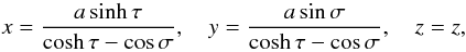 (1)where a is a
constant. Both τ and σ-coordinate lines are circles, all
τ-coordinate lines passing through the points
x = ±a on the x-axis. The equations of the
boundaries of the left and right tube are τ = −τL
and τ = τR respectively. The tube radii and the
distance between their axes, d, are expressed in terms of
τL and τR by
(1)where a is a
constant. Both τ and σ-coordinate lines are circles, all
τ-coordinate lines passing through the points
x = ±a on the x-axis. The equations of the
boundaries of the left and right tube are τ = −τL
and τ = τR respectively. The tube radii and the
distance between their axes, d, are expressed in terms of
τL and τR by  (2)The interior of each tube
consists of the core region and the annulus attached to the tube boundary. The internal boundary
of the left and right annulus are determined by
τ = −τL − ℓL and
τ = τR + ℓR
respectively. The sketch of the equilibrium is given in Fig. 1.
(2)The interior of each tube
consists of the core region and the annulus attached to the tube boundary. The internal boundary
of the left and right annulus are determined by
τ = −τL − ℓL and
τ = τR + ℓR
respectively. The sketch of the equilibrium is given in Fig. 1.
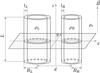 |
Fig. 1 Sketch of the equilibrium configuration. |
Outside the tubes the density is ρe. In the core of the left tube
and right tube it is ρL and ρR
respectively,
ρe < ρL,R.
In the left and right annulus it decreases from ρL to
ρe and from ρR to
ρe. Summarizing, we have 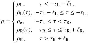 (3)were
 is monotonically decreasing and
  monotonically increasing function,
  ,
,
 ,
,
 ,
and
,
and  .
.
In what follows we use the approximation of cold plasma. The plasma motion is described by the
system of linearized viscous MHD equations, ![Mathematical equation: \begin{equation} \rho\frac{\partial^2\vec{\xi}}{\partial t^2} = \frac1{\mu_0}(\nabla\times\vec{b})\times\vec{B} + \frac\partial{\partial t}\big[\nabla(\tilde{\eta}\nabla\cdot\vec{\xi}) -\nabla\times(\tilde{\eta}\nabla\times\vec{\xi})\big], \label{eq:2.4} \end{equation}](/articles/aa/full_html/2011/01/aa15525-10/aa15525-10-eq36.png) (4)
(4) (5)Here
ξ is the plasma displacement, b
the magnetic field perturbation,
B = Bez
the equilibrium magnetic field, ez the
unit vector in the z-direction, μ0 the magnetic
permeability of free space, and
(5)Here
ξ is the plasma displacement, b
the magnetic field perturbation,
B = Bez
the equilibrium magnetic field, ez the
unit vector in the z-direction, μ0 the magnetic
permeability of free space, and  the dynamics
viscosity. In the solar corona the viscosity tensor is strongly anisotropic, so that, strictly
speaking, we have to use the full Braginskii’s expression for the viscosity tensor (Braginskii 1965). For typical coronal parameters the
coefficient of compressional viscosity in the Braginskii’s expression is by many orders of
magnitude larger than the coefficient of shear viscosity. However we take viscosity into account
only to remove the singularity at the Alfvén resonant position, so that the viscosity is only
important in a thin dissipative layer embracing the Alfvén magnetic resonant surface. In spite
of the fact that, in general, the compressional viscosity strongly dominates the shear
viscosity, it does not affect the plasma motion in the Alfvén dissipative layer (Ofman et al. 1994; Erdélyi
& Goossens 1995). Hence, when writing Eq. (4), we have taken only the shear viscosity into account, and
is the
coefficient of shear viscosity.
the dynamics
viscosity. In the solar corona the viscosity tensor is strongly anisotropic, so that, strictly
speaking, we have to use the full Braginskii’s expression for the viscosity tensor (Braginskii 1965). For typical coronal parameters the
coefficient of compressional viscosity in the Braginskii’s expression is by many orders of
magnitude larger than the coefficient of shear viscosity. However we take viscosity into account
only to remove the singularity at the Alfvén resonant position, so that the viscosity is only
important in a thin dissipative layer embracing the Alfvén magnetic resonant surface. In spite
of the fact that, in general, the compressional viscosity strongly dominates the shear
viscosity, it does not affect the plasma motion in the Alfvén dissipative layer (Ofman et al. 1994; Erdélyi
& Goossens 1995). Hence, when writing Eq. (4), we have taken only the shear viscosity into account, and
is the
coefficient of shear viscosity.
Equations (4) and (5) have to be supplemented by boundary conditions.
Since the magnetic field lines are frozen in a dense immovable photospheric plasma at
z = ±L/2, the plasma displacement in the
direction orthogonal to the z-direction,
ξ ⊥ , has to vanish at
z = ±L/2. Hence  (6)The system of Eqs. (4) and (5) and the boundary condition (6) will
be used in the next section to study the damping of kink oscillations.
(6)The system of Eqs. (4) and (5) and the boundary condition (6) will
be used in the next section to study the damping of kink oscillations.
3. Derivation of expression for oscillation decrement
The aim of this section is to derive the expression for oscillation decrement. To do this we solve the linearized MHD equations separately in the outer region, in the core regions of the magnetic tubes, and in the annuluses, and then match the solutions.
Let us transform the system of Eqs. (4)
and (5). First of all we rewrite these equations
as ![Mathematical equation: \begin{equation} \rho\frac{\partial^2\vec{\xi}}{\partial t^2} = -\nabla P + \frac B{\mu_0}\frac{\partial\vec{b}}{\partial z} + \frac\partial{\partial t}[\nabla(\tilde{\eta}\nabla\cdot\vec{\xi}) -\nabla\times(\tilde{\eta}\nabla\times\vec{\xi})], \label{eq:3.1} \end{equation}](/articles/aa/full_html/2011/01/aa15525-10/aa15525-10-eq46.png) (7)
(7) (8)where
P = b·B/μ0
is the perturbation of magnetic pressure. Viscosity can be neglected everywhere except the
dissipative layer where there are large gradients in the τ-direction. This, in
particular, implies that we can neglect the derivatives of
in comparison
with the derivatives of ξ. Hence, we can use the approximate
relation
(8)where
P = b·B/μ0
is the perturbation of magnetic pressure. Viscosity can be neglected everywhere except the
dissipative layer where there are large gradients in the τ-direction. This, in
particular, implies that we can neglect the derivatives of
in comparison
with the derivatives of ξ. Hence, we can use the approximate
relation  (9)Substituting this relation in
Eq. (4) we immediately obtain that
ξz = 0, i.e.
ξ = ξ ⊥ . Taking this
result into account, substituting Eq. (8)
in (7), and using Eq. (9) we transform Eq. (7) to
(9)Substituting this relation in
Eq. (4) we immediately obtain that
ξz = 0, i.e.
ξ = ξ ⊥ . Taking this
result into account, substituting Eq. (8)
in (7), and using Eq. (9) we transform Eq. (7) to  (10)where
 is the square of
the Alfvén speed. Taking the scalar product of Eq. (8) with B yields
is the square of
the Alfvén speed. Taking the scalar product of Eq. (8) with B yields  (11)Since the coefficients in
Eqs. (10) and (11) are independent of z, we can Fourier-analyze these
equations with respect to z. In what follows we consider only the fundamental
mode with respect to z. To satisfy the boundary conditions (6) we take ξ
proportional to cos(πz/L). Then it follows
from Eq. (11) that P is also
proportional to cos(πz/L). We are looking
for solutions in the form of dissipative eigenmodes. In accordance with this we take
ξ and P proportional to
exp(− ωt) with complex ω. As a result Eq. (10) reduces to
(11)Since the coefficients in
Eqs. (10) and (11) are independent of z, we can Fourier-analyze these
equations with respect to z. In what follows we consider only the fundamental
mode with respect to z. To satisfy the boundary conditions (6) we take ξ
proportional to cos(πz/L). Then it follows
from Eq. (11) that P is also
proportional to cos(πz/L). We are looking
for solutions in the form of dissipative eigenmodes. In accordance with this we take
ξ and P proportional to
exp(− ωt) with complex ω. As a result Eq. (10) reduces to 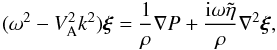 (12)where
k = π/L. Equation (11) remains the same.
(12)where
k = π/L. Equation (11) remains the same.
Let us now write Eqs. (10), and (11) in bi-cylindrical coordinates
τ,σ,z. In these coordinates
ξ = (ξτ,ξσ,0),
 (13)
(13)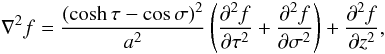 (14)
(14)![Mathematical equation: \begin{eqnarray} \nabla\cdot\vec{g} &=& \frac{(\cosh\tau - \cos\sigma)^2}a \bigg[\frac{\partial}{\partial\tau}\left(\frac{g_\tau} {\cosh\tau - \cos\sigma}\right) \nonumber\\ \label{eq:3.9}&& +\, \frac{\partial}{\partial\sigma} \left(\frac{g_\sigma}{\cosh\tau - \cos\sigma}\right)\bigg] + \frac{\partial g_z}{\partial z}, \end{eqnarray}](/articles/aa/full_html/2011/01/aa15525-10/aa15525-10-eq65.png) (15)
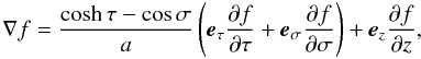
(15)![Mathematical equation: \begin{eqnarray} \nabla\times\vec{g} &=& \vec{e}_\tau\left(\frac{\cosh\tau - \cos\sigma}a \frac{\partial g_z}{\partial\sigma} - \frac{\partial g_\sigma}{\partial z}\right)\nonumber\\ &&- \,\vec{e}_\sigma\left(\frac{\cosh\tau - \cos\sigma}a \frac{\partial g_z}{\partial\tau} - \frac{\partial g_\tau}{\partial z}\right)\nonumber\\ &&+ \,\vec{e}_z\frac{(\cosh\tau - \cos\sigma)^2}a \bigg[\frac{\partial}{\partial\tau}\left(\frac{g_\sigma} {\cosh\tau - \cos\sigma}\right) \nonumber\\ \label{eq:3.10}&& -\, \frac{\partial}{\partial\sigma} \left(\frac{g_\tau}{\cosh\tau - \cos\sigma}\right)\bigg], \end{eqnarray}](/articles/aa/full_html/2011/01/aa15525-10/aa15525-10-eq66.png) (16)(see,
e.g., Korn & Korn 1961). Here f
and g are arbitrary scalar and vector-function respectively, and
eτ and
eσ are the unit vectors in the
τ and σ directions respectively. Using the identity
∇2ξ = ∇∇·ξ − ∇ × ∇ × ξ
and Eqs. (13), (15) and (16) we can easily
obtain the expression for ∇2ξ. Repeat that viscosity is
only important in a thin dissipative layer embracing the resonant magnetic surface. In this
layer there are large gradients only in the τ-direction. This observation
enables us to neglect all terms in the expression for
∇2ξ but the term proportional to the second derivative
of ξ with respect to τ. As a result we arrive at
the approximate expression
(16)(see,
e.g., Korn & Korn 1961). Here f
and g are arbitrary scalar and vector-function respectively, and
eτ and
eσ are the unit vectors in the
τ and σ directions respectively. Using the identity
∇2ξ = ∇∇·ξ − ∇ × ∇ × ξ
and Eqs. (13), (15) and (16) we can easily
obtain the expression for ∇2ξ. Repeat that viscosity is
only important in a thin dissipative layer embracing the resonant magnetic surface. In this
layer there are large gradients only in the τ-direction. This observation
enables us to neglect all terms in the expression for
∇2ξ but the term proportional to the second derivative
of ξ with respect to τ. As a result we arrive at
the approximate expression 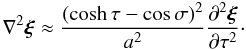 (17)In the
limit of very small viscosity the damping rate of oscillations due to resonant absorption is
independent of the particular value of (e.g. Goossens & Ruderman 1995). In particular, we can
assume any dependence of on
τ and σ under the only restriction that the characteristic
scale of variation of is much larger
than the thickness of the dissipative layer. To simplify the calculations as much as possible we
take
(17)In the
limit of very small viscosity the damping rate of oscillations due to resonant absorption is
independent of the particular value of (e.g. Goossens & Ruderman 1995). In particular, we can
assume any dependence of on
τ and σ under the only restriction that the characteristic
scale of variation of is much larger
than the thickness of the dissipative layer. To simplify the calculations as much as possible we
take  (18)where
ν is a constant. Now we can write the system of Eqs. (11) and (12) in components,
(18)where
ν is a constant. Now we can write the system of Eqs. (11) and (12) in components, ![Mathematical equation: \begin{eqnarray} P &=& -\frac1a\rho V_{\rm A}^2(\cosh\tau - \cos\sigma)^2 \nonumber\\ \label{eq:3.13}&&\times\, \bigg[\frac{\partial}{\partial\tau}\left(\frac{\vec{\xi}_\tau} {\cosh\tau - \cos\sigma}\right) + \frac{\partial}{\partial\sigma} \left(\frac{\vec{\xi}_\sigma}{\cosh\tau - \cos\sigma}\right)\bigg], \end{eqnarray}](/articles/aa/full_html/2011/01/aa15525-10/aa15525-10-eq76.png) (19)
(19) (20)
(20) (21)These
equations will be used in the next subsections to derive the expression for the decrement.
(21)These
equations will be used in the next subsections to derive the expression for the decrement.
3.1. Solution in the outer and core regions
In the outer and core regions we neglect viscosity. The density in these regions is constant.
Eliminating ξτ and
ξσ from Eqs. (19)–(21) with the terms
describing viscosity neglected we obtain the equation for P,  (22)In what follows we assume
that the tube length L is much larger than the characteristic size of the system in the
directions orthogonal to the tube axes. We can take this characteristic size equal to
d. Hence, we assume that
d/L = ϵ ≪ 1. Now we
easily obtain that, since
ω ~ kVA, the ratio of the last
term in Eq. (22) to the first and second term
is of the order of ϵ2. Neglecting this small term we obtain the
approximate equation for P,
(22)In what follows we assume
that the tube length L is much larger than the characteristic size of the system in the
directions orthogonal to the tube axes. We can take this characteristic size equal to
d. Hence, we assume that
d/L = ϵ ≪ 1. Now we
easily obtain that, since
ω ~ kVA, the ratio of the last
term in Eq. (22) to the first and second term
is of the order of ϵ2. Neglecting this small term we obtain the
approximate equation for P,  (23)It follows from Eq. (1) that
τ2 + σ2 → 0 far from the magnetic
tubes, i.e. when x2 + y2 → ∞. The
general solution to Eq. (23) can be looked for
in the form of Fourier expansion with respect to σ. However we are only
interested in the kink oscillations, so that we look for the solution to Eq. (23) in the form
(23)It follows from Eq. (1) that
τ2 + σ2 → 0 far from the magnetic
tubes, i.e. when x2 + y2 → ∞. The
general solution to Eq. (23) can be looked for
in the form of Fourier expansion with respect to σ. However we are only
interested in the kink oscillations, so that we look for the solution to Eq. (23) in the form  (24)where
σ0 is a constant and Φ(τ) a function to be
determined. The second term on the right-hand side of this expression is introduced to satisfy
the condition that P → 0 as
τ2 + σ2 → 0. When
τ → ±∞ we have x = ±a and
y → 0. This implies that the solution to Eq. (23) has to be bounded when τ → ±∞. Then we immediately
obtain that
(24)where
σ0 is a constant and Φ(τ) a function to be
determined. The second term on the right-hand side of this expression is introduced to satisfy
the condition that P → 0 as
τ2 + σ2 → 0. When
τ → ±∞ we have x = ±a and
y → 0. This implies that the solution to Eq. (23) has to be bounded when τ → ±∞. Then we immediately
obtain that  (25)where
C1, C2, CL
and CR are arbitrary constants. Now, using Eq. (20) with the last term neglected, we arrive at
(25)where
C1, C2, CL
and CR are arbitrary constants. Now, using Eq. (20) with the last term neglected, we arrive at
 (26)where
  (27)Since
P and ξ has to be continuous at the annulus
boundaries, Eq. (24) is also valid in the
annuluses. Then it follows from Eq. (20) that
Eq. (26) is also valid in the annuluses.
Finally, it follows from Eq. (20) that we can
write ξσ as
(27)Since
P and ξ has to be continuous at the annulus
boundaries, Eq. (24) is also valid in the
annuluses. Then it follows from Eq. (20) that
Eq. (26) is also valid in the annuluses.
Finally, it follows from Eq. (20) that we can
write ξσ as  (28)Substituting Eqs. (26) and (28) in Eq. (19) we obtain
 (29)It is easy to see that this
equation is inconsistent with Eq. (24). However
let us estimate the order of terms in Eq. (29).
It follows from Eq. (21) that
(29)It is easy to see that this
equation is inconsistent with Eq. (24). However
let us estimate the order of terms in Eq. (29).
It follows from Eq. (21) that
 .
Then it immediately follows that the ratio of the right-hand side of Eq. (29) to its left-hand side is of the order of
ϵ2, so that the right-hand side can be neglected in the long
wavelength approximation. As a result Eq. (29)
is simplified to
.
Then it immediately follows that the ratio of the right-hand side of Eq. (29) to its left-hand side is of the order of
ϵ2, so that the right-hand side can be neglected in the long
wavelength approximation. As a result Eq. (29)
is simplified to  (30)Obviously this equation does
not contradict to Eq. (24). This analysis
clearly shows that the expressions for P and ξ
given by Eqs. (24), (26) and (28) can be used only in the long wavelength approximation.
(30)Obviously this equation does
not contradict to Eq. (24). This analysis
clearly shows that the expressions for P and ξ
given by Eqs. (24), (26) and (28) can be used only in the long wavelength approximation.
3.2. Solution in the dissipative layer
When the tubes are homogeneous Van Doorsselaere et al. 13 has shown that, in the long wavelength approximation, there are two
eigenfrequencies of kink modes, ω− and
ω+,
ω− < ω+.
All systems of two parallel magnetic tubes can be separated in two classes: standard and
anomalous. In standard systems  (31)In anomalous systems
 (32)In
what follows assume that the annuluses are thin,
ℓL ≪ RL and
ℓR ≪ RR. In that case the main effect
due to the presence of the annuluses is the resonant damping of a kink mode, the real part of
the frequency only being slightly modified. Hence, the real part of eigenfrequency of a damped
dissipative eigenmode is approximately equal to either ω− or
ω+. The resonance conditions for the left and right tubes are
written as
(32)In
what follows assume that the annuluses are thin,
ℓL ≪ RL and
ℓR ≪ RR. In that case the main effect
due to the presence of the annuluses is the resonant damping of a kink mode, the real part of
the frequency only being slightly modified. Hence, the real part of eigenfrequency of a damped
dissipative eigenmode is approximately equal to either ω− or
ω+. The resonance conditions for the left and right tubes are
written as  (33)where
τ = τAL and
τ = τAR are the equations of the resonant
surfaces in the right and left annulus respectively, and ω is equal either
ω− or ω+. Then it follows from
Eq. (31) that, in a standard system, there is
the resonant surface both in the left and right annulus for both the slower
(ω = ω−) and faster
(ω = ω+) eigenmodes. On the other hand, it
follows from Eq. (32) that, in an anomalous
system, there is the resonant surface both in the left and right annulus only for the faster
eigenmode. For the slower eigenmode there is only one resonant surface. This surface is in the
denser tube, i.e. in the tube with the smaller Alfvén speed in the core region.
(33)where
τ = τAL and
τ = τAR are the equations of the resonant
surfaces in the right and left annulus respectively, and ω is equal either
ω− or ω+. Then it follows from
Eq. (31) that, in a standard system, there is
the resonant surface both in the left and right annulus for both the slower
(ω = ω−) and faster
(ω = ω+) eigenmodes. On the other hand, it
follows from Eq. (32) that, in an anomalous
system, there is the resonant surface both in the left and right annulus only for the faster
eigenmode. For the slower eigenmode there is only one resonant surface. This surface is in the
denser tube, i.e. in the tube with the smaller Alfvén speed in the core region.
Let us study the wave motion in the dissipative layer embracing a resonant surface. The analysis is the same for the dissipative layers in the left and right tubes, so that we will drop the subscripts “L” and “R” in what follows.
Substituting Eqs. (24), (26) and (28) in Eqs. (20) and (21) we obtain  (34)
(34) (35)In what
follows we will see that the ration of the decrement γ to the real part of the
eigenfrequency is of the order of ℓ/R ≪ 1.
This implies that we can use the approximation
(35)In what
follows we will see that the ration of the decrement γ to the real part of the
eigenfrequency is of the order of ℓ/R ≪ 1.
This implies that we can use the approximation  (36)where
either ω0 = ω− or
ω0 = ω+. We also can substitute
ω0 for ω in the coefficient at the second
derivative in Eqs. (34) and (35). The equation of the resonant magnetic surface
is τ = τA, where τA is
defined by
kVA(τA) = ω0.
The characteristic scale of variation of VA in the annulus is
ℓ, while the thickness of the dissipative layer is much smaller than
ℓ. This implies that, in the dissipative layer we can use the approximation
(36)where
either ω0 = ω− or
ω0 = ω+. We also can substitute
ω0 for ω in the coefficient at the second
derivative in Eqs. (34) and (35). The equation of the resonant magnetic surface
is τ = τA, where τA is
defined by
kVA(τA) = ω0.
The characteristic scale of variation of VA in the annulus is
ℓ, while the thickness of the dissipative layer is much smaller than
ℓ. This implies that, in the dissipative layer we can use the approximation
 (37)It is convenient to
introduce the new variable
(37)It is convenient to
introduce the new variable  (38)Note that
 , where
Re = ω0L2/ν
is the Reynolds number. For typical coronal conditions Re is so
large that δ ≪ 1.
, where
Re = ω0L2/ν
is the Reynolds number. For typical coronal conditions Re is so
large that δ ≪ 1.
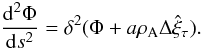
Using Eqs. (36)–(38) we rewrite Eqs. (30), (34) and (35) in the new variables as  (39)
(39) (40)
(40)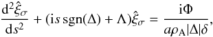 (41)where
Λ = 2ω0γ/δ |Δ|
and ρA is the density calculated at the resonant position, i.e.
(41)where
Λ = 2ω0γ/δ |Δ|
and ρA is the density calculated at the resonant position, i.e.
 .
Now we differentiate Eq. (40), subtract
Eq. (41) multiplied by δ from
the result, and use Eq. (39) to obtain
.
Now we differentiate Eq. (40), subtract
Eq. (41) multiplied by δ from
the result, and use Eq. (39) to obtain
 (42)Since δ ≪ 1
it follows from this equation that the variation of Φ in the dissipative layer is very small,
and we can take Φ ≈ const. = Φ(τA) in the dissipative layer. This
result is well known in the theory of resonant MHD waves in planar and cylindrical geometry
(e.g. Hollweg 1987; Goossens at al. 1995). With Φ = const. Eq. (41) coincides, with the accuracy up to the notation, with the corresponding equation
considered by 12. Hence, we can us the results obtained
by these authors and immediately write
(42)Since δ ≪ 1
it follows from this equation that the variation of Φ in the dissipative layer is very small,
and we can take Φ ≈ const. = Φ(τA) in the dissipative layer. This
result is well known in the theory of resonant MHD waves in planar and cylindrical geometry
(e.g. Hollweg 1987; Goossens at al. 1995). With Φ = const. Eq. (41) coincides, with the accuracy up to the notation, with the corresponding equation
considered by 12. Hence, we can us the results obtained
by these authors and immediately write 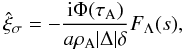 (43)where
 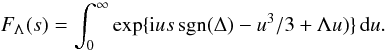 (44)Substituting Eq. (43) in (39) and using Eq. (44) we obtain
 (45)where
  (46)The functions
FΛ and GΛ were first introduced by
10.
(46)The functions
FΛ and GΛ were first introduced by
10.
Let us introduce the jump of a function f(s) across the
dissipative layer, ![Mathematical equation: \begin{eqnarray*} [f] = \lim_{s \to \infty}\{f(s) - f(-s)\}.\nonumber \end{eqnarray*}](/articles/aa/full_html/2011/01/aa15525-10/aa15525-10-eq154.png) Since
we take Φ = const. in the dissipative layer we immediately obtain
Since
we take Φ = const. in the dissipative layer we immediately obtain ![Mathematical equation: \begin{equation} [\Phi] = 0. \label{eq:3.2.17} \end{equation}](/articles/aa/full_html/2011/01/aa15525-10/aa15525-10-eq155.png) (47)It is straightforward to
obtain [G] = iπsgn(Δ). It follows from this result and
Eq. (45) that
(47)It is straightforward to
obtain [G] = iπsgn(Δ). It follows from this result and
Eq. (45) that ![Mathematical equation: \begin{equation} [\hat{\xi}_\tau] = -\frac{{\rm i}\pi\Phi(\tau_{\rm A})}{a\rho_{\rm A}|\Delta|}\cdot \label{eq:3.2.18} \end{equation}](/articles/aa/full_html/2011/01/aa15525-10/aa15525-10-eq157.png) (48)Equations (47) and (48) will be used in the next subsection to connect the solutions at the left and the
right of the dissipative layer.
(48)Equations (47) and (48) will be used in the next subsection to connect the solutions at the left and the
right of the dissipative layer.
3.3. Variation of pressure and velocity across the annuluses
In this subsections we calculate the variations of P and
 across the annuluses. We give the detailed calculation of these variations in the left annulus,
and then present only the final results for the right annulus. Since we assume that
ℓ ≪ 1, in our calculations we will keep only the linear terms with respect to
ℓ, while we will neglect quadratic terms and terms of the higher order.
across the annuluses. We give the detailed calculation of these variations in the left annulus,
and then present only the final results for the right annulus. Since we assume that
ℓ ≪ 1, in our calculations we will keep only the linear terms with respect to
ℓ, while we will neglect quadratic terms and terms of the higher order.
To calculate the variation of
across the annuluses we use Eqs. (30)
and (35). Since Eq. (35) is used outside the dissipative layer, we
neglect the last term on its right-hand side. Since, in accordance with Eq. (47) Φ does not jump across the dissipative layer,
and we neglect the variation of Φ when calculating ,
we take Φ = Φ(τAL) ≡ ΦAL in Eq. (35) (recall that
τ = τAL is the equation of the resonant magnetic
surface in the left annulus). Since the imaginary part of ω is of the order of
ℓ we also substitute ω0 for ω.
Then we easily obtain ![Mathematical equation: \begin{equation} \hat{\xi}_\tau = \hat{\xi}_\tau(-\tau_{\rm L}-\ell_{\rm L}) + \frac{\Phi_{\rm AL}}a \int_{-\tau_{\rm L}-\ell_{\rm L}}^\tau \frac{{\rm d}\tilde{\tau}} {\bar{\rho}_{\rm L}(\tilde{\tau})\left[\omega_0^2 - k^2 V_{\rm A}^2(\tilde{\tau})\right]}, \label{eq:3.3.1} \end{equation}](/articles/aa/full_html/2011/01/aa15525-10/aa15525-10-eq161.png) (49)for
−τL − ℓL ≤ τ < τAL,
and
(49)for
−τL − ℓL ≤ τ < τAL,
and ![Mathematical equation: \begin{equation} \hat{\xi}_\tau = \hat{\xi}_\tau(-\tau_{\rm L}) - \frac{\Phi_{\rm AL}}a \int_\tau^{-\tau_{\rm L}} \frac{{\rm d}\tilde{\tau}} {\bar{\rho}_{\rm L}(\tilde{\tau})\left[\omega_0^2 - k^2 V_{\rm A}^2(\tilde{\tau})\right]}, \label{eq:3.3.2} \end{equation}](/articles/aa/full_html/2011/01/aa15525-10/aa15525-10-eq163.png) (50)for
τAL < τ < ℓL − τL.
Equations (49) and (50) clearly show that
has a logarithmic singularity at τ = τAL in a
complete agreement with the general theory of resonant MHD waves.
(50)for
τAL < τ < ℓL − τL.
Equations (49) and (50) clearly show that
has a logarithmic singularity at τ = τAL in a
complete agreement with the general theory of resonant MHD waves.
Equations (49) and (50) give the ideal solution outside the dissipative
layer in the left annulus. Now we match this solution with the solution in the dissipative
layer in two overlap layers at the left and right of the dissipative layer. In these layers
both the ideal and dissipative solution are valid. It follows from the matching condition that
the limit of any quantity defined in the dissipative layer as s → ±∞ has to
coincide with the limit of the same quantity defined outside the dissipative layer as
τ → ±0. It follows from this condition that we can give another formula for
the jump of function f across the dissipative layer,
![Mathematical equation: \begin{eqnarray*} [f] = \lim_{\varepsilon \to +0}\{f(\tau_{\rm AL} + \varepsilon) - f(\tau_{\rm AL} - \varepsilon)\}.\nonumber \end{eqnarray*}](/articles/aa/full_html/2011/01/aa15525-10/aa15525-10-eq167.png) Then
we obtain from Eqs. (49) and (50) that
Then
we obtain from Eqs. (49) and (50) that ![Mathematical equation: \begin{equation} [\hat{\xi}_\tau] = \delta\hat{\xi}_{\tau {\rm L}} - \frac{\Phi_{\rm AL}}a {\cal P}\int_{-\tau_{\rm L}-\ell_{\rm L}}^{-\tau_{\rm L}} \frac{{\rm d}\tau} {\bar{\rho}_{\rm L}(\tau)\left[\omega_0^2 - k^2 V_{\rm A}^2(\tau)\right]}, \label{eq:3.3.3} \end{equation}](/articles/aa/full_html/2011/01/aa15525-10/aa15525-10-eq168.png) (51)where
(51)where
 indicates the principal Cauchy part of the integral, and
  (52)Comparing Eqs. (48) and (51) yields
 ![Mathematical equation: \begin{equation} \delta\hat{\xi}_{\tau {\rm L}} = \frac{\Phi_{\rm AL}}a \left({\cal P}\int_{-\tau_{\rm L}-\ell_{\rm L}}^{-\tau_{\rm L}}\frac{{\rm d}\tau} {\bar{\rho}_{\rm L}(\tau)\left[\omega_0^2 - k^2 V_{\rm A}^2(\tau)\right]} - \frac{{\rm i}\pi}{\rho_{\rm AL}|\Delta_{\rm L}|}\right)\cdot \label{eq:3.3.5} \end{equation}](/articles/aa/full_html/2011/01/aa15525-10/aa15525-10-eq171.png) (53)To
calculate the variation of Φ across the annulus we use Eq. (34) with the last term on the left-hand side neglected and
ω0 substituted for ω. Since, in accordance with
Eq. (53) the variation of
across the annulus is of the order of ℓL, we neglect it when
calculating the variation of Φ and substitute
(53)To
calculate the variation of Φ across the annulus we use Eq. (34) with the last term on the left-hand side neglected and
ω0 substituted for ω. Since, in accordance with
Eq. (53) the variation of
across the annulus is of the order of ℓL, we neglect it when
calculating the variation of Φ and substitute  for
in Eq. (34). Then we immediately obtain
for
in Eq. (34). Then we immediately obtain
![Mathematical equation: \begin{equation} \delta\Phi_{\rm L} = a\hat{\xi}_\tau(-\tau_{\rm L})\int_{-\tau_{\rm L}-\ell_{\rm L}}^{-\tau_{\rm L}} \bar{\rho}_{\rm L}(\tau)\left[\omega_0^2 - k^2 V_{\rm A}^2(\tau)\right]\,{\rm d}\tau, \label{eq:3.3.6} \end{equation}](/articles/aa/full_html/2011/01/aa15525-10/aa15525-10-eq174.png) (54)where
(54)where  (55)Repeating the same
calculation but for the right annulus yields
(55)Repeating the same
calculation but for the right annulus yields ![Mathematical equation: \begin{equation} \delta\hat{\xi}_{\tau {\rm R}} = \frac{\Phi_{\rm AR}}a \left(\frac{{\rm i}\pi}{\rho_{\rm AR}|\Delta_{\rm R}|} - {\cal P}\int_{\tau_{\rm R}}^{\tau_{\rm R}+\ell_{\rm R}}\frac{{\rm d}\tau} {\bar{\rho}_{\rm R}(\tau)\left[\omega_0^2 - k^2 V_{\rm A}^2(\tau)\right]}\right), \label{eq:3.3.8} \end{equation}](/articles/aa/full_html/2011/01/aa15525-10/aa15525-10-eq176.png) (56)
(56)![Mathematical equation: \begin{equation} \delta\Phi_{\rm R} = -a\hat{\xi}_\tau(\tau_{\rm R})\int_{\tau_{\rm R}}^{\tau_{\rm R}+\ell_{\rm R}} \bar{\rho}_{\rm R}(\tau)\left[\omega_0^2 - k^2 V_{\rm A}^2(\tau)\right]\,{\rm d}\tau, \label{eq:3.3.9} \end{equation}](/articles/aa/full_html/2011/01/aa15525-10/aa15525-10-eq177.png) (57)where
(57)where  (58)
(58)
3.4. Matching solutions and calculation of decrements
Now we match the solutions in the core regions with the solution outside the tubes. For this
we calculate the variations of  and Φ across the annuluses using Eqs. (25)
and (27), and then compare them with those
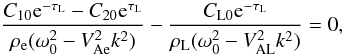
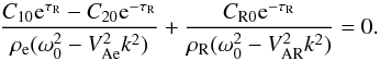
given by Eqs. (52)–(58). As a result we obtain
and Φ across the annuluses using Eqs. (25)
and (27), and then compare them with those
given by Eqs. (52)–(58). As a result we obtain ![Mathematical equation: \begin{eqnarray} C_1 {\rm e}^{-\tau_{\rm L}} + C_2 {\rm e}^{\tau_{\rm L}} &-& C_{\rm L} {\rm e}^{-\tau_{\rm L}-\ell_{\rm L}} = \frac{C_1 {\rm e}^{-\tau_{\rm L}} - C_2 {\rm e}^{\tau_{\rm L}}} {\rho_{\rm e}(\omega_0^2 - V_{\rm Ae}^2 k^2)} \nonumber\\ \label{eq:3.4.1}&\times& \int_{-\tau_{\rm L}-\ell_{\rm L}}^{-\tau_{\rm L}} \bar{\rho}_{\rm L}(\tau)[\omega_0^2 - k^2 V_{\rm A}^2(\tau)]\,{\rm d}\tau, \end{eqnarray}](/articles/aa/full_html/2011/01/aa15525-10/aa15525-10-eq180.png) (59)
(59)![Mathematical equation: \begin{eqnarray} C_1 {\rm e}^{\tau_{\rm R}} + C_2 {\rm e}^{-\tau_{\rm R}} &-& C_{\rm R} {\rm e}^{-\tau_{\rm R}-\ell_{\rm R}} = \frac{C_1 {\rm e}^{\tau_{\rm R}} - C_2 {\rm e}^{-\tau_{\rm R}}} {\rho_{\rm e}(\omega_0^2 - V_{\rm Ae}^2 k^2)} \nonumber\\ \label{eq:3.4.2}&\times& \int_{\tau_{\rm R}}^{\tau_{\rm R}+\ell_{\rm R}} \bar{\rho}_{\rm L}(\tau)[\omega_0^2 - k^2 V_{\rm A}^2(\tau)]\,{\rm d}\tau, \end{eqnarray}](/articles/aa/full_html/2011/01/aa15525-10/aa15525-10-eq181.png) (60)
(60)![Mathematical equation: \begin{eqnarray} \frac{C_1 {\rm e}^{-\tau_{\rm L}} - C_2 {\rm e}^{\tau_{\rm L}}} {\rho_{\rm e}(\omega^2 - V_{\rm Ae}^2 k^2)} &-& \frac{C_{\rm L} {\rm e}^{-\tau_{\rm L}-\ell_{\rm L}}}{\rho_{\rm L}(\omega^2 - V_{\rm AL}^2 k^2)} = (C_1 {\rm e}^{-\tau_{\rm L}} + C_2 {\rm e}^{\tau_{\rm L}}) \nonumber\\ \label{eq:3.4.3}&\hphantom{x}& \hspace*{-13mm} \times\, \left({\cal P}\int_{-\tau_{\rm L}-\ell_{\rm L}}^{-\tau_{\rm L}}\frac{{\rm d}\tau} {\bar{\rho}_{\rm L}(\tau)[\omega_0^2 - k^2 V_{\rm A}^2(\tau)]} - \frac{{\rm i}\pi}{\rho_{\rm AL}|\Delta_{\rm L}|}\right), \end{eqnarray}](/articles/aa/full_html/2011/01/aa15525-10/aa15525-10-eq182.png) (61)
(61)![Mathematical equation: \begin{eqnarray} \frac{C_1 {\rm e}^{\tau_{\rm R}} - C_2 {\rm e}^{-\tau_{\rm R}}} {\rho_{\rm e}(\omega^2 - V_{\rm Ae}^2 k^2)} &+& \frac{C_{\rm R} {\rm e}^{-\tau_{\rm R}-\ell_{\rm R}}}{\rho_{\rm R}(\omega^2 - V_{\rm AR}^2 k^2)} = (C_1 {\rm e}^{\tau_{\rm R}} + C_2 {\rm e}^{-\tau_{\rm R}}) \nonumber\\ \label{eq:3.4.4}&\hphantom{x}& \hspace*{-13mm} \times\, \left(\frac{{\rm i}\pi}{\rho_{\rm AR}|\Delta_{\rm R}|} - {\cal P}\int_{\tau_{\rm R}}^{\tau_{\rm R}+\ell_{\rm R}}\frac{{\rm d}\tau} {\bar{\rho}_{\rm R}(\tau)[\omega_0^2 - k^2 V_{\rm A}^2(\tau)]}\right)\cdot \end{eqnarray}](/articles/aa/full_html/2011/01/aa15525-10/aa15525-10-eq183.png) (62)When
deriving Eqs. (59)–(62) we have used the formulae obtained with the aid
of Eqs. (25) and (27),
(62)When
deriving Eqs. (59)–(62) we have used the formulae obtained with the aid
of Eqs. (25) and (27),  (63)The
system of Eqs. (59)–(62) is the system of linear homogeneous algebraic
equations. It has a nontrivial solution only if its determinant is zero. This condition gives
the dispersion equation that relates ω and k.
(63)The
system of Eqs. (59)–(62) is the system of linear homogeneous algebraic
equations. It has a nontrivial solution only if its determinant is zero. This condition gives
the dispersion equation that relates ω and k.
The ratios of the right-hand sides of Eqs. (59)–(62) to their left-hand sides are
of the order of either ℓL ≪ 1 or
ℓR ≪ 1. This observation enables us to use the regular perturbation
method to solve the system of Eqs. (59)–(62). In accordance with this method we look for the
solution in the form  (64)where
the second terms on the right-hand sides of these expressions are much smaller than the first
terms. In addition, we write
(64)where
the second terms on the right-hand sides of these expressions are much smaller than the first
terms. In addition, we write  (65)where
|ω1| ≪ |ω0| .
(65)where
|ω1| ≪ |ω0| .
3.4.1. Zero-order approximation
Substituting Eqs. (64) and (65) in Eqs. (59)–(62), keeping only the
largest terms and neglecting the right-hand sides we obtain in the zero-order approximation
 (66)
(66) (67)
(67) (68)
(68) (69)This system has a non-trivial
solution only when its determinant is zero. This gives the dispersion equation determining
ω0 as a function of k. The system of Eqs. (66)–(69) is the same as the system of Eqs. (29) in Van Doorsselaere et al. 13, so that we can use the results obtained by these
authors. It follows from their analysis that the solution to the dispersion equation is
(69)This system has a non-trivial
solution only when its determinant is zero. This gives the dispersion equation determining
ω0 as a function of k. The system of Eqs. (66)–(69) is the same as the system of Eqs. (29) in Van Doorsselaere et al. 13, so that we can use the results obtained by these
authors. It follows from their analysis that the solution to the dispersion equation is
 , where
  (70)
(70)![Mathematical equation: \begin{equation} \zeta_{\rm L}=\frac{\rho_{\rm L}}{\rho_{\rm e}}, \quad \zeta_{\rm R}=\frac{\rho_{\rm R}}{\rho_{\rm e}}, \quad E = \exp[-(\tau_{\rm L}+\tau_{\rm R})], \label{eq:3.4.13} \end{equation}](/articles/aa/full_html/2011/01/aa15525-10/aa15525-10-eq197.png) (71)
(71) (72)Note
that, while Luna et al. 4 found four different
eigenfrequencies, we obtained only two, ω+ and
ω−. As it has been already suggested by Van Doorsselaere et al.
13, the most probable cause of this difference is that
we have neglected the wave dispersion related to the fact that the ratio of the tube radius to
its length is small but finite.
(72)Note
that, while Luna et al. 4 found four different
eigenfrequencies, we obtained only two, ω+ and
ω−. As it has been already suggested by Van Doorsselaere et al.
13, the most probable cause of this difference is that
we have neglected the wave dispersion related to the fact that the ratio of the tube radius to
its length is small but finite.
Luna et al. 4 gave an excellent physical explanation why there are high- and low-frequency modes (in their case two high- and two low-frequency modes) of the kink oscillations of two parallel magnetic tubes. Not repeating their explanation we only mention that it is based on the analysis of the plasma motion outside the tubes. In the high-frequency modes this plasma motion provides an additional restoring force thus increasing the oscillation frequency. In the low-frequency modes it reduces the restoring force thus decreasing the oscillation frequency.
3.4.2. First-order approximation
In the first order approximation we collect terms proportional to
C11, C21,
CL1, CR1,
ω1, ℓL or
ℓR in Eqs. (59)–(62). As a result we obtain
![Mathematical equation: \begin{eqnarray} C_{11}{\rm e}^{-\tau_{\rm L}} &+& C_{21}{\rm e}^{\tau_{\rm L}} - C_{\rm L1}{\rm e}^{-\tau_{\rm L}} = \frac{C_{10}{\rm e}^{-\tau_{\rm L}} - C_{20}{\rm e}^{\tau_{\rm L}}} {\rho_{\rm e}(\omega_0^2 - V_{\rm Ae}^2 k^2)} \nonumber\\ \label{eq:3.4.15}&\times& \int_{-\tau_{\rm L}-\ell_{\rm L}}^{-\tau_{\rm L}} \bar{\rho}_{\rm L}(\tau)\left[\omega_0^2 - k^2 V_{\rm A}^2(\tau)\right]\,{\rm d}\tau - C_{\rm L0}\ell_{\rm L} {\rm e}^{-\tau_{\rm L}}, \end{eqnarray}](/articles/aa/full_html/2011/01/aa15525-10/aa15525-10-eq205.png) (73)
(73)![Mathematical equation: \begin{eqnarray} C_{11}{\rm e}^{\tau_{\rm R}} &+& C_{21}{\rm e}^{-\tau_{\rm R}} - C_{\rm R1}{\rm e}^{-\tau_{\rm R}} = \frac{C_{10}{\rm e}^{\tau_{\rm R}} - C_{20}{\rm e}^{-\tau_{\rm R}}} {\rho_{\rm e}(\omega_0^2 - V_{\rm Ae}^2 k^2)} \nonumber\\ \label{eq:3.4.16}&\times& \int_{\tau_{\rm R}}^{\tau_{\rm R}+\ell_{\rm R}} \bar{\rho}_{\rm R}(\tau)\left[\omega_0^2 - k^2 V_{\rm A}^2(\tau)\right]\,{\rm d}\tau - C_{\rm R0}\ell_{\rm R} {\rm e}^{-\tau_{\rm R}}, \end{eqnarray}](/articles/aa/full_html/2011/01/aa15525-10/aa15525-10-eq206.png) (74)
(74)![Mathematical equation: \begin{eqnarray} \frac{C_{11}{\rm e}^{-\tau_{\rm L}} - C_{21}{\rm e}^{\tau_{\rm L}}}{\rho_{\rm e}(\omega_0^2 - V_{\rm Ae}^2 k^2)} &-& \frac{C_{\rm L1}{\rm e}^{-\tau_{\rm L}}} {\rho_{\rm L}(\omega_0^2 - V_{\rm AL}^2 k^2)} = (C_{10}{\rm e}^{-\tau_{\rm L}} + C_{20}{\rm e}^{\tau_{\rm L}}) \nonumber\\ &\hphantom{x}& \hspace*{-20mm} \times\, \left({\cal P}\int_{-\tau_{\rm L}-\ell_{\rm L}}^{-\tau_{\rm L}}\frac{{\rm d}\tau} {\bar{\rho}_{\rm L}(\tau)\left[\omega_0^2 - k^2 V_{\rm A}^2(\tau)\right]} - \frac{{\rm i}\pi}{\rho_{\rm AL}|\Delta_{\rm L}|}\right) \nonumber\\ &\hphantom{x}& \hspace*{-20mm} +\, 2\omega_0\omega_1\left(\frac{C_{10}{\rm e}^{-\tau_{\rm L}} - C_{20}{\rm e}^{\tau_{\rm L}}}{\rho_{\rm e}(\omega_0^2 - V_{\rm Ae}^2 k^2)^2} - \frac{C_{\rm L0}{\rm e}^{-\tau_{\rm L}}}{\rho_{\rm L}(\omega_0^2 - V_{\rm AL}^2 k^2)^2} \right) \nonumber\\ \label{eq:3.4.17}&\hphantom{x}& \hspace*{-20mm} -\, \frac{C_{\rm L0}\ell_{\rm L} {\rm e}^{-\tau_{\rm L}}} {\rho_{\rm L}(\omega_0^2 - V_{\rm AL}^2 k^2)}, \end{eqnarray}](/articles/aa/full_html/2011/01/aa15525-10/aa15525-10-eq207.png) (75)
(75)![Mathematical equation: \begin{eqnarray} \frac{C_{11}{\rm e}^{\tau_{\rm R}} - C_{21}{\rm e}^{-\tau_{\rm R}}}{\rho_{\rm e}(\omega_0^2 - V_{\rm Ae}^2 k^2)} &+& \frac{C_{\rm R1}{\rm e}^{-\tau_{\rm R}}} {\rho_{\rm R}(\omega_0^2 - V_{\rm AR}^2 k^2)} = (C_{10}{\rm e}^{\tau_{\rm R}} + C_{20}{\rm e}^{-\tau_{\rm R}}) \nonumber\\ &\hphantom{x}& \hspace*{-20mm} \times\, \left(\frac{{\rm i}\pi}{\rho_{\rm AR}|\Delta_{\rm R}|} - {\cal P}\int_{\tau_{\rm R}}^{\tau_{\rm R}+\ell_{\rm R}}\frac{{\rm d}\tau} {\bar{\rho}_{\rm R}(\tau)\left[\omega_0^2 - k^2 V_{\rm A}^2(\tau)\right]}\right) \nonumber\\ &\hphantom{x}& \hspace*{-20mm} +\, 2\omega_0\omega_1\left(\frac{C_{10}{\rm e}^{\tau_{\rm R}} - C_{20}{\rm e}^{-\tau_{\rm R}}}{\rho_{\rm e}(\omega_0^2 - V_{\rm Ae}^2 k^2)^2} + \frac{C_{\rm R0}{\rm e}^{-\tau_{\rm R}}}{\rho_{\rm R}(\omega_0^2 - V_{\rm AR}^2 k^2)^2} \right) \nonumber\\ \label{eq:3.4.18}&\hphantom{x}& \hspace*{-20mm} +\, \frac{C_{\rm R0}\ell_{\rm R} {\rm e}^{-\tau_{\rm R}}} {\rho_{\rm R}(\omega_0^2 - V_{\rm AR}^2 k^2)}\cdot \end{eqnarray}](/articles/aa/full_html/2011/01/aa15525-10/aa15525-10-eq208.png) (76)Equations (73)–(76) constitute the system of linear inhomogeneous algebraic equations. The
homogeneous counterpart of this system coincides with the system of Eqs. (66)–(69), so that it has a non-trivial solution. This means that its determinant is zero,
so that the system of inhomogeneous Eqs. (73)–(76) is solvable only if its
right-hand side satisfies the compatibility condition.
(76)Equations (73)–(76) constitute the system of linear inhomogeneous algebraic equations. The
homogeneous counterpart of this system coincides with the system of Eqs. (66)–(69), so that it has a non-trivial solution. This means that its determinant is zero,
so that the system of inhomogeneous Eqs. (73)–(76) is solvable only if its
right-hand side satisfies the compatibility condition.
At this point calculations are getting increasingly complicated. For the sake of simplicity
we restrict further analysis to the case of two identical tubes. In accordance with this we
drop the subscripts “L” and “R” and introduce the notation  (77)For this particular case
 (78)Using Eqs. (68), (69), (77) and (78) we obtain that the compatibility condition for
the system of Eqs. (73)–(76) reads
(78)Using Eqs. (68), (69), (77) and (78) we obtain that the compatibility condition for
the system of Eqs. (73)–(76) reads ![Mathematical equation: \begin{eqnarray} 2\omega_\pm\omega_1 &+& \rho_{\rm e} V_{\rm Ae}^4 k^4 \frac{(\zeta - 1)^2(1 - {\rm e}^{-4\tau_0})(1 \pm {\rm e}^{-2\tau_0})} {[(\zeta + 1) \mp {\rm e}^{-2\tau_0}(\zeta - 1)]^3} \nonumber\\ \label{eq:3.4.21}&\times& \left(\frac{{\rm i}\pi}{\rho_{\rm A}|\Delta|} - {\cal P}\int_{\tau_0}^{\tau_0 + \ell}\frac{{\rm d}\tau} {\bar{\rho}(\omega_\pm^2 - k^2 V_{\rm Ae}^4)}\right) = 0. \end{eqnarray}](/articles/aa/full_html/2011/01/aa15525-10/aa15525-10-eq211.png) (79)It
follows from this equation that
(79)It
follows from this equation that  (80)where
 ![Mathematical equation: \begin{eqnarray} \bar{\omega}_{1\pm} &=& \frac{\rho_{\rm e} V_{\rm Ae}^4 k^4(\zeta - 1)^2 (1 - {\rm e}^{-4\tau_0})(1 \pm {\rm e}^{-2\tau_0})}{2\omega_\pm[(\zeta + 1) \mp {\rm e}^{-2\tau_0}(\zeta - 1)]^3} \nonumber\\ \label{eq:3.4.23}&& \times\, \,{\cal P}\int_{\tau_0}^{\tau_0 + \ell} \frac{{\rm d}\tau}{\bar{\rho}(\omega_\pm^2 - k^2 V_{\rm Ae}^4)}, \end{eqnarray}](/articles/aa/full_html/2011/01/aa15525-10/aa15525-10-eq213.png) (81)
(81)![Mathematical equation: \begin{equation} \gamma_\pm = \frac{\pi\rho_{\rm e} V_{\rm Ae}^4 k^4(\zeta - 1)^2 (1 - {\rm e}^{-4\tau_0})(1 \pm {\rm e}^{-2\tau_0})}{2\omega_\pm\rho_{\rm A}|\Delta| \left[(\zeta + 1) \mp {\rm e}^{-2\tau_0}(\zeta - 1)\right]^3}\cdot \label{eq:3.4.24} \end{equation}](/articles/aa/full_html/2011/01/aa15525-10/aa15525-10-eq214.png) (82)The
quantity
(82)The
quantity  is not important because it gives only small correction to the oscillation frequency. The
important quantity is the decrement γ that determines the oscillation damping
rate due to resonant absorption. In the next section we will study the dependence of
γ on the parameters of the equilibrium.
is not important because it gives only small correction to the oscillation frequency. The
important quantity is the decrement γ that determines the oscillation damping
rate due to resonant absorption. In the next section we will study the dependence of
γ on the parameters of the equilibrium.
4. Investigation of oscillation damping
In this section we study the dependence of the decrement γ on the relative
distance between the tube axes, d/R, and on
the density contract ζ. In what follows we assume that
 is a linear function of τ, so that
  (83)Recall that the Alfvén
resonant position τA is determined by the equation
kVA(τA) = ω ± .
It follows from this equation that
(83)Recall that the Alfvén
resonant position τA is determined by the equation
kVA(τA) = ω ± .
It follows from this equation that 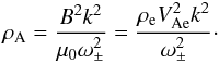 (84)Using
this result we obtain
(84)Using
this result we obtain  (85)Using
Eqs. (78), (84) and (85) we obtain from
Eq. (82) that
(85)Using
Eqs. (78), (84) and (85) we obtain from
Eq. (82) that ![Mathematical equation: \begin{equation} \gamma_\pm = \frac{\pi\ell \omega_\pm (\zeta - 1)(1 - {\rm e}^{-4\tau_0})(1 \pm {\rm e}^{-2\tau_0})} {8\left[(\zeta + 1) \mp {\rm e}^{-2\tau_0}(\zeta - 1)\right]}\cdot \label{eq:4.4} \end{equation}](/articles/aa/full_html/2011/01/aa15525-10/aa15525-10-eq223.png) (86)It was
found in studies of resonant damping of kink oscillations of single magnetic loops that the
decrement is proportional to the ratio of the inhomogeneous annulus thickness to the loop radius
(see, e.g., Ruderman & Roberts 2002; Goossens
et al. 2002; Goossens
et al. 2006; Ruderman & Erdélyi 2009). To
compare the damping rate of kink oscillations of two parallel loops with that of a single loop
it would be convenient to write the expression for γ ± in the same
form. We see from Eq. (86) that
γ ± is proportional to ℓ. However
ℓ is equal to the ratio of the annulus thickness to the loop radius only when
the distance between the loop axes is much larger than the loop radius. It would be desirable to
express ℓ in terms of this ratio in the general case. The difficulty is that,
in general, the annulus thickness is not constant. Rather it is a function of
σ. To overcome this difficulty we introduce the mean thickness of the annulus.
The equations of the external and internal boundaries of the annulus in Cartesian coordinates
are given by Eq. (1) with τ
substituted by τ0 and
τ0 + ℓ respectively. Then, taking into account
that ℓ ≪ τ0, we obtain that the annulus thickness
at fixed σ is given by the approximate formula
(86)It was
found in studies of resonant damping of kink oscillations of single magnetic loops that the
decrement is proportional to the ratio of the inhomogeneous annulus thickness to the loop radius
(see, e.g., Ruderman & Roberts 2002; Goossens
et al. 2002; Goossens
et al. 2006; Ruderman & Erdélyi 2009). To
compare the damping rate of kink oscillations of two parallel loops with that of a single loop
it would be convenient to write the expression for γ ± in the same
form. We see from Eq. (86) that
γ ± is proportional to ℓ. However
ℓ is equal to the ratio of the annulus thickness to the loop radius only when
the distance between the loop axes is much larger than the loop radius. It would be desirable to
express ℓ in terms of this ratio in the general case. The difficulty is that,
in general, the annulus thickness is not constant. Rather it is a function of
σ. To overcome this difficulty we introduce the mean thickness of the annulus.
The equations of the external and internal boundaries of the annulus in Cartesian coordinates
are given by Eq. (1) with τ
substituted by τ0 and
τ0 + ℓ respectively. Then, taking into account
that ℓ ≪ τ0, we obtain that the annulus thickness
at fixed σ is given by the approximate formula ![Mathematical equation: \begin{equation} \delta(\sigma) = \ell\left[\left(\frac{\partial x}{\partial\tau}\right)^2 + \left(\frac{\partial y}{\partial\tau}\right)^2\right]^{1/2} = \frac{a\ell}{\cosh\tau_0 - \cos\sigma}\cdot \label{eq:4.5} \end{equation}](/articles/aa/full_html/2011/01/aa15525-10/aa15525-10-eq228.png) (87)The mean
annulus thickness is given by
(87)The mean
annulus thickness is given by 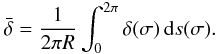 (88)The
square of the elementary length along the annulus boundary is given by
(88)The
square of the elementary length along the annulus boundary is given by ![Mathematical equation: \begin{eqnarray} {\rm d}s^2 = {\rm d}x^2 + {\rm d}y^2 &=& \left[\left(\frac{\partial x} {\partial\sigma}\right)^2 + \left(\frac{\partial y} {\partial\sigma}\right)^2\right]{\rm d}\sigma^2 \nonumber\\ \label{eq:4.7} &=& \frac{a^2\,{\rm d}\sigma^2}{(\cosh\tau_0 - \cos\sigma)^2}\cdot \end{eqnarray}](/articles/aa/full_html/2011/01/aa15525-10/aa15525-10-eq230.png) (89)In
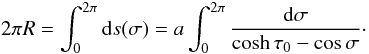
particular, it follows from this result that the length of the annulus boundary is given by
(89)In
particular, it follows from this result that the length of the annulus boundary is given by
 (90)Using Eqs. (87) and (89) we obtain from Eq. (88) that
 (91)Substituting in Eq. (90)
R = a/sinhτ0
and differentiating the obtained identity with respect to τ0 we
obtain
(91)Substituting in Eq. (90)
R = a/sinhτ0
and differentiating the obtained identity with respect to τ0 we
obtain  (92)Substituting this result in
Eq. (91) yields
(92)Substituting this result in
Eq. (91) yields  (93)Using this result we rewrite
Eq. (86) as
(93)Using this result we rewrite
Eq. (86) as ![Mathematical equation: \begin{equation} \gamma_\pm = \frac{\pi\bar{\delta}\omega_\pm (\zeta - 1)(1 \pm {\rm e}^{-2\tau_0})(1 - {\rm e}^{-2\tau_0})^2} {8R\left[(\zeta + 1) \mp {\rm e}^{-2\tau_0}(\zeta - 1)\right]}\cdot \label{eq:4.12} \end{equation}](/articles/aa/full_html/2011/01/aa15525-10/aa15525-10-eq236.png) (94)This
formula is quite convenient for comparison with the damping rate obtained for a single loop.
First of all we note that the damping rate is proportional to the annulus thickness. The same
result was obtained for a single magnetic tube in the thin boundary layer approximation (e.g.
Ruderman & Roberts 2002; Goossens et al. 2006). When τ0 → ∞ we obtain
d/R → ∞. In this case the loops oscillate
independently, and the annulus thickness is constant,
(94)This
formula is quite convenient for comparison with the damping rate obtained for a single loop.
First of all we note that the damping rate is proportional to the annulus thickness. The same
result was obtained for a single magnetic tube in the thin boundary layer approximation (e.g.
Ruderman & Roberts 2002; Goossens et al. 2006). When τ0 → ∞ we obtain
d/R → ∞. In this case the loops oscillate
independently, and the annulus thickness is constant,  .
When τ0 → ∞ we obtain
.
When τ0 → ∞ we obtain  and
and 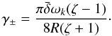 (95)This result is in a complete
agreement with that obtained for a single loop (see, e.g., Goossens et al. 2002; Ruderman & Erdélyi 2009).
The dependence of
(95)This result is in a complete
agreement with that obtained for a single loop (see, e.g., Goossens et al. 2002; Ruderman & Erdélyi 2009).
The dependence of  on d/R and ζ is shown in
in Figs. 2 and 3
respectively.
on d/R and ζ is shown in
in Figs. 2 and 3
respectively.
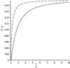 |
Fig. 2 The dependence of the decrement γ on the distance between the loop axes d for ζ = 3. The solid and dashed curves correspond to the slower (ω = ω−) and faster (ω = ω+) kink oscillations. |
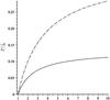 |
Fig. 3 The dependence of the decrement γ on the density contrast ζ for d/R = 2.5. The solid and dashed curves correspond to the slower (ω = ω−) and faster (ω = ω+) kink oscillations. |
5. Summary and conclusions
In this paper we have studied the damping of kink oscillations of the system of two parallel straight magnetic tubes. The density has been assumed to be constant outside the tubes and in the core regions of the tubes, while it was varying in the radial direction in thin annuluses near the tube boundaries. As a result there are resonant positions in the annuluses. There is one resonant position in each annulus in a system of standard type both for modes with lower and higher frequencies, while in a system of anomalous type there are still two resonant positions for modes with higher frequencies, but only one resonant position in the annulus in a denser tube for modes with lower frequencies.
The assumption that the annuluses are thin enabled us to use the regular perturbation method to study the damping of kink oscillations due to resonant absorption. In the zero-order approximation we reproduced the results of studying kink oscillations of two homogeneous tubes obtained by Van Doorsselaere et al. 13. In the first-order approximation we calculated the damping rate due to resonant absorption. At this stage calculations are getting increasingly complicated, so that we restricted our analysis to the case of identical magnetic tubes.
The main results concerning the damping of oscillations can be summarized as follows. We can
see from Fig. 2 that, for ζ = 3, the
decrements of both slower and faster kink modes are monotonically increasing functions of
d/R. Taking into account that
d/R = coshτ0,
i.e. d/R is a monotonically increasing
function of τ0, it is straightforward to show that the same result
is valid for any value ζ > 1. Hence, the interaction
between the tubes reduces the efficiency of resonant damping. Formally,
γ ± → 0 as
d/R → 2. However, the assumption that the
annuluses are thin implies that not only  ,
but also
,
but also  is much smaller than the distance between the tube boundaries. This second restriction is
equivalent to
is much smaller than the distance between the tube boundaries. This second restriction is
equivalent to  .
.
Another important conclusion concerning the damping rate is that γ−/ω− < γ+/ω+, i.e. the damping time of slower oscillations is larger than that of faster oscillations. For example, for ζ = 3 and d/R = 2.5, the damping time of slower oscillations is more than twice larger than that of faster oscillations. At present we cannot provide a physical explanation to this result. Finally, similar to the case of a single tube, the damping time is an increasing function of the density contrast ζ.
It is interesting to compare our results with those obtained by 1. In their study of resonantly damped kink oscillations of the system of two parallel slabs these authors found that the properties of kink oscillations of this system and the damping time are practically the same as of a single slab with the equivalent parameters. In this sense the properties of kink oscillations of a system of two tubes are quite different from those of two-slab system. While 1 found only one fundamental eigenfrequency of kink oscillations, we found two of them and, as we know from the study by Luna et al. 4, actually there are four eigenfrequencies if the wave dispersion is taken into account. We also found that the damping rate due to resonant absorption is sufficiently reduced by the tube interaction. This difference between our results and those by 1 is not very surprising. As we have already noted, the properties of kink oscillations of single slabs and tubes are quite different. It is then natural to expect a substantial difference in properties of kink oscillations of two-tube and two-slab systems.
One final note is that the result that the damping rate decreases when the tube separation decreases should be treated with caution. The point is that, when studying the damping rate, we fixed the average thickness of the annuluses where the density decreases from its value inside the tubes to its external value.
However the shape of annuluses changes when the tube separation decreases. Their thickness is getting larger in the outer parts of the tubes and smaller in the inner part. It is possible that the damping rate decrease is related to this change of annulus shape. To clarify this point one needs to study the effect of annulus shape on the damping rate. In this respect we note that this problem has not been addressed yet even in the case of a single magnetic tube. So it is an interesting problem for future studies.
Acknowledgments
M.S.R. acknowledges the support by an STFC grant. D.R. acknowledges the support by an STFC postgraduate fellowship.
References
- Andries, J., Goossens, M., Hollweg, J. V., Arregui, I., & Van Doorsselaere, T. 2005, A&A, 430, 1109 [NASA ADS] [CrossRef] [EDP Sciences] [Google Scholar]
- Arregui, I., Terradas, J., Oliver, R., & Ballester, J. L. 2007, A&A, 466, 1145 [NASA ADS] [CrossRef] [EDP Sciences] [Google Scholar]
- Arregui, I., Terradas, J., Oliver, R., & Ballester, J. L. 2008, ApJ, 674, 1179 [NASA ADS] [CrossRef] [Google Scholar]
- Aschwanden, M. J. 2005, ApJ, 634, L193 [NASA ADS] [CrossRef] [Google Scholar]
- Aschwanden, M. J., & Nightingale, R. W. 2005, ApJ, 633, 499 [NASA ADS] [CrossRef] [Google Scholar]
- Aschwanden, M. J., Fletcher, L., Schrijver, C. J., & Alexander, D. 1999, ApJ, 520, 880 [NASA ADS] [CrossRef] [Google Scholar]
- Aschwanden, M. J., De Pontieu, B., Schrijver, C. J., & Tilte, A. M. 2002, Sol. Phys., 206, 99 [NASA ADS] [CrossRef] [Google Scholar]
- Braginskii, S. I., 1965, in Review of Plasma Physics, ed. A. V. Leontovich (New York: Consultants Bureau), 1, 205 [Google Scholar]
- Dymova, M. V., & Ruderman, M. S. 2006, A&A, 457, 1059 [NASA ADS] [CrossRef] [EDP Sciences] [Google Scholar]
- Erdélyi, R., & Goossens, M. 1995, A&A 294, 575 [NASA ADS] [Google Scholar]
- Goossens, M., & Ruderman, M. S. 1995, Phys. Scripta, T60, 171 [Google Scholar]
- Goossens, M., Ruderman, M. S., & Hollweg, J. V. 1995, Sol. Phys., 157, 75 [NASA ADS] [CrossRef] [Google Scholar]
- Goossens, M., Andries, J., & Aschwanden, M. J. 2002, A&A, 394, L39 [NASA ADS] [CrossRef] [EDP Sciences] [Google Scholar]
- Goossens, M., Andries, J., & Arregui, I. 2006, Phil. Trans. R. Soc. A, 364, 433 [NASA ADS] [CrossRef] [Google Scholar]
- Hollweg, J. V. 1987, ApJ, 312, 880 [NASA ADS] [CrossRef] [Google Scholar]
- Korn, G., & Korn, T. 1961, Mathematical handbook for scientists and engineers (New York: McGraw-Hill) [Google Scholar]
- Luna, M., Terradas, J., Oliver, R., & Ballester, J. L. 2008, ApJ, 676, 717 [NASA ADS] [CrossRef] [Google Scholar]
- Luna, M., Terradas, J., Oliver, R., & Ballester, J. L. 2009, ApJ, 692, 1582 [NASA ADS] [CrossRef] [Google Scholar]
- Luna, M., Terradas, J., Oliver, R., & Ballester, J. L. 2010, ApJ, 716, 1371 [NASA ADS] [CrossRef] [Google Scholar]
- Martens, P. C. H., Cirtain, J. W., & Schmelz, J. T. 2002, ApJ, 577, L115 [NASA ADS] [CrossRef] [Google Scholar]
- Morton, R. J., & Erdelyi, R. 2009, ApJ, 707, 750 [NASA ADS] [CrossRef] [Google Scholar]
- Nakariakov, V. M., Ofman, L., DeLuca, E. E., Roberts, B., & Davila, J. M. 1999, Science, 285, 862 [NASA ADS] [CrossRef] [PubMed] [Google Scholar]
- Ofman, L. 2005, Adv. Space Res., 36, 1572 [NASA ADS] [CrossRef] [Google Scholar]
- Ofman, L. 2009, ApJ, 694, 502 [NASA ADS] [CrossRef] [Google Scholar]
- Ofman, L., & Aschwanden, M. J. 2002, ApJ, 576, L153 [NASA ADS] [CrossRef] [Google Scholar]
- Ofman, L., Davila, J. M., & Steinolfson, R. S. 1994, ApJ, 421, 360 [NASA ADS] [CrossRef] [Google Scholar]
- Robertson, D., Ruderman, M. S., & Taroyan Y. 2010, A&A, 515, A33 [NASA ADS] [CrossRef] [EDP Sciences] [Google Scholar]
- Ruderman, M. S., & Erdélyi, R. 2009, Space. Sci. Rev., 149, 199 [CrossRef] [Google Scholar]
- Ruderman, M. S., & Roberts, R. 2002, ApJ, 577, 475 [NASA ADS] [CrossRef] [Google Scholar]
- Ruderman, M. S., Tirry, W., & Goossens, M. 1995, J. Plasma Phys., 54, 129 [NASA ADS] [CrossRef] [Google Scholar]
- Schmelz, J. T., Cirtain, J. W., Beene, J. E., et al. 2003, Adv. Space Res., 32, 1109 [NASA ADS] [CrossRef] [Google Scholar]
- Schmelz, J. T., Nasraoui, K., Richardson, V. L., et al. 2005, ApJ, 627, L81 [NASA ADS] [CrossRef] [Google Scholar]
- Schrijver, C. J., Aschwanden, M. J., & Tilte, A. M. 2002, Sol. Phys., 206, 69 [NASA ADS] [CrossRef] [Google Scholar]
- Terradas, J., Arregui, I., Oliver, R., et al. 2008, ApJ, 679, 1611 [NASA ADS] [CrossRef] [Google Scholar]
- Tirry, W. J., & Goossens, M. 1996, ApJ, 471, 501 [NASA ADS] [CrossRef] [Google Scholar]
- Van Doorsselaere, T., Ruderman, M. S., & Robertson, D. 2008, A&A, 485, 849 [NASA ADS] [CrossRef] [EDP Sciences] [Google Scholar]
- Verwichte, E., Nakariakov, V., Ofman, L., & DeLuca, E. E. 2004, Sol. Phys. 223, 77 [NASA ADS] [CrossRef] [Google Scholar]
All Figures
|
Fig. 1 Sketch of the equilibrium configuration. |
| In the text | |
|
Fig. 2 The dependence of the decrement γ on the distance between the loop axes d for ζ = 3. The solid and dashed curves correspond to the slower (ω = ω−) and faster (ω = ω+) kink oscillations. |
| In the text | |
|
Fig. 3 The dependence of the decrement γ on the density contrast ζ for d/R = 2.5. The solid and dashed curves correspond to the slower (ω = ω−) and faster (ω = ω+) kink oscillations. |
| In the text | |
Current usage metrics show cumulative count of Article Views (full-text article views including HTML views, PDF and ePub downloads, according to the available data) and Abstracts Views on Vision4Press platform.
Data correspond to usage on the plateform after 2015. The current usage metrics is available 48-96 hours after online publication and is updated daily on week days.
Initial download of the metrics may take a while.