© ESO, 2010

1. Introduction

It is well known since the 1980s that the spectra of low-mass X-ray binaries (LMXBs) hosting a neutron star (NS) can be described up to about 30 keV by a two-component model representing the contribution from different emitting regions of the system. However, the interpretation of the spectra is not unique as demonstrated by the variety of different models used over the years. Before the BeppoSAX and RXTE era, two concurring models were the standard to describe X-ray emission in LMXBs. In the so-called “eastern model” (Mitsuda et al. 1984, 1989) the spectra were fitted by the sum of a soft blackbody (BB) emission (actually modeled by a multi-color disk BB spectrum) attributed to the accretion disk, plus a hotter simple or Comptonized BB claimed to originate close to the NS surface. On the other hand, in the “western model” interpretation (White et al. 1986, 1988), the direct BB component was attributed to the NS surface, while an unsaturated Comptonization spectrum was thought to originate from a hot corona above the inner accretion disk, which supplies most of the soft seed photons for Comptonization. Indeed, even after the advent of BeppoSAX and RXTE, the persistent emission of NS LMXBs was described by the sum of a BB component plus a thermal Comptonization (TC) spectrum, usually described by the XSPEC Comptt model (Titarchuk 1994, hereafter T94). Despite the significant improvement in our knowledge of the source spectral properties by means of the broadband observations, the BB+TC model was subjected to a dichotomy. Indeed, both cases provide generally equally acceptable good fits, no matter whether the temperature of the direct BB spectrum (kT_bb) is lower (e.g., Di Salvo et al. 2000a,b, 2001; Oosterbroek et al. 2001; Gierliński & Done 2002; Lavagetto et al. 2004; Paizis et al. 2005) or higher (e.g., Paizis et al. 2005; Farinelli et al. 2007; Farinelli et al. 2008, hereafter F08) than that of the thermally Comptonized seed photons (kT_s).

The consequences of these results were the interpretation of the BB emission as owing either to the accretion disk (kT_bb < kT_s) or to the NS surface (kT_bb > kT_s). Moreover, in addition to the persistent X-ray emission, BeppoSAX (e.g., Di Salvo et al. 2000a, 2002) RXTE (D’Amico et al. 2001; Di Salvo et al. 2006) and later also INTEGRAL (Paizis et al. 2006, hereafter P06) allowed the possibility to discover a transient powerlaw (PL) X-ray emission above 30 keV in bright NS LMXBs.

Motivated by the need to put some order and give an unified scenario of the different NS system spectral states, Paizis et al. (2006, hereafter P06) performed a systematic observational campaign with the ISGRI (20–200 keV) monitor onborad INTEGRAL. Using long-term average spectra and including former INTEGRAL results on GX 354–0 (Falanga et al. 2006), P06 classified NS LMXBs into four main states: the hard/PL, low/hard, intermediate and soft. The high-energy (>20 keV) spectra in different sources were interpreted by P06 as the result of the interplay between thermal and bulk Comptonization processes, whose relative efficiency is ultimately dictated by the mass-accretion rate. At high energies (where the direct BB component is negligible), the hard/PL state spectra can be fitted with a simple PL component; the low/hard spectra by a TC spectrum of soft (≲1 keV) BB-like photons off an electron population with kT_e ~20−30 keV and τ₀ ≲ 3; the intermediate state spectra by a TC spectrum with kT_e ~3−5 keV and τ₀ ≳ 5 plus a PL component with photon index Γ ~2−3; the soft state spectra by a TC component similar to the intermediate state, but without the high-energy X-ray tail.

From the observational point of view, the quantities directly measurable in the data are the cut-off energy E_c of the dominating TC bump and the spectral slope, parameterized through the energy index α (=   Γ−1). For pure TC spectra, α is tightly correlated with the plasma temperature kT_e and optical depth τ₀ (Sunyaev & Titarchuk 1980; Titarchuk & Lyubarskij 1995, hereafter TL95), while in the presence of a converging flow (bulk motion), the shape of the velocity field also determines the emerging spectral slope (Titarchuk et al. 1997; Laurent & Titarchuk 1999, F08). In mathematical terms, α represents the index of the system Green’s function (GF), namely as it responds to monochromatic line injection. The resulting emerging spectrum is then obtained as a convolution of the GF with the input seed photon spectrum. We also emphasize that the hard/PL, hard and soft states spectra of NS LMXBs are characterized by only one Comptonization index (see Fig. 4 in P06). In the first case, its value is interpreted as a result of a mixed thermal plus bulk Comptonization effect, while in the latter two cases α is derived from pure TC. On the other hand, the intermediate state spectra show two Comptonization indexes, one is related to the persistent TC component and the other one characterizes the transient PL-like hard X-ray emission.

In Sect. 2 we give an overview of the theoretical and observational issues related to spectral evolution in X-ray binary systems hosting a NS or a black hole (BH) and outline the differences among the two classes of sources. We subsequently report on results related to the observed TC index α for a sample of NS sources. In Sect. 3 we propose a theoretical model based on diffusion formalism for radiative transfer in order to explain the observational results. In Sect. 4 we discuss the comparison between theory and data, while in Sect. 5 we draw our conclusions and give future observational perspects.

2. Spectral index evolution in neutron star systems

Starting from the considerations of the previous section, it is important to make a comparison between the index evolution in accreting BH and NS sources. The spectral state of BH sources may be generally divided into low/hard state (LHS), where the spectrum is dominated by a TC component with electron temperature kT_e ~60–100 keV, intermediate state (IS), with a BB bump (presumably coming from the accretion disk) and a superposed PL high-energy component, and high/soft state (HSS) where the BB component is even stronger and the PL emission is steeper.

Actually, in BH systems generally one high energy photon index Γ is observed (see e.g. recent results on GRS 1915+015 by Titarchuk & Seifina 2009; and Shaposhnikov & Titarchuk 2009) and its value evolves with the source mass-accretion rate. The latter, which is not a direct observable quantity, may be inferred in an indirect way by means of the the normalization of the disk flux N_disk. In a Γ vs. N_disk/Quasi Periodic Oscillation (QPO) frequency diagram, it was found (Shaposhnikov & Titarchuk 2009; Titarchuk & Seifina 2009; Montanari et al. 2009) that the photon index progressively increases from Γ ~1.6–1.8 as the source moves from the LHS to the HSS, until it reaches saturation around Γ ~2.2−2.4 (depending on the source). This interpretation of the observed BH spectra was performed using the BMC model (Titarchuk et al. 1997), whose emerging spectral shape is $\mathit{F}\mathrm{\left(}\mathit{E}\mathrm{\right)}\mathrm{=}\frac{{\mathit{C}}_{\mathit{N}}}{\mathit{A}\mathrm{+}\mathrm{1}}\mathrm{\left[}\mathit{BB}\mathrm{\right(}\mathit{E}\mathrm{)}\mathrm{+}\mathit{A}\mathrm{\times }\mathit{G}\mathrm{(}\mathit{E,}{\mathit{E}}_{\mathrm{0}}\mathrm{)}\mathrm{\ast }\mathit{BB}\mathrm{(}{\mathit{E}}_{\mathrm{0}}\mathrm{\left)}\mathrm{\right]}\mathit{.}$(1)In Eq. (1), the first term on the right-hand side represents the direct seed photon BB-like spectrum, while the second one gives its modification due to Comptonization (convolution with GF). The hardness of the spectrum is dictated by the energy index α of the GF which, in BMC, is a broken-PL with G(E,E₀) ∝ E^α + 3 for E < E₀ and G(E,E₀) ∝ E^−α for E > E₀, where E₀ is the monochromatic input energy. It is important to keep in mind that the GF in BMC does not contain the exponential spectral rollover, so when the latter is observed in the X-ray spectrum of a source, it can be taken into account by multiplying the model with an exponential e-folding factor  ∝ e^−E/E_c.

The index saturation observed in BH sources as they move to the HSS finds a natural explanation in the framework of a bulk-dominated scenario (see mathematical proof of this statement in e.g. Titarchuk & Seifina 2009). Moreover, when the sources are in the LHS the points in the Γ vs. N_disk/QPO diagram form a plateau around Γ ~1.5 before the rising phase. This clear mapping of the energy (or photon) index evolution is possible in BH sources because they are generally strongly variable and their X-ray spectrum allows for a one-to-one correspondence between the spectral state and the energy index α (or Γ) using spectral modeling according to Eq. (1). One of the advantages of BMC model is that it is a generic Comptonization model, because it allows to map the spectral evolution of sources through the Comptonization index α, which is a direct measurable quantity, no matter what the underlying physical conditions. The theoretical interpretation of the source spectral formation is postponed at another time.

For NS sources however, the situation is less straightforward. Most variable sources do exhibit pure TC spectra, with the electron temperature kT_e progressively decreasing and the optical depth τ₀ increasing, respectively, when they move from the hard to the soft state. Examples for this are GX 354–0 (Falanga et al. 2006) or 4U 1608–52 (Gierliński & Done 2002). On the other hand, bright LMXBs of the GX class such as the classical six known Z sources (Sco X–1, GX 17+2, Cyg X–2, GX 340+0, GX 5–1 and GX 349+2) and, more recently, GX 13+1, show only a small evolution of their persistent X-ray continuum (dominated by the strong TC bump with kT_e ~3–5 keV and τ₀ ≫ 1). They are additionally characterized by a transient hard X-ray PL-like component (intermediate state).

Other persistently bright sources such as GX 3+1, GX 9+1, and GX 9+9 have only been observed in the soft state without evidence of hard X-ray tails. Indeed, a mapping of the evolution of the transient hard X-ray tail of NS sources in the intermediate state has not been yet possible because of the insufficient statistics available at high energies. Some attempts (Di Salvo et al. 2000a, 2002, 2006) were actually undertaken to establish changes in the intensity of the transient hard X-ray tail by fitting it with a simple PL and, when statistics was poor, fixing the index by allowing to vary only its flux. But nothing could be concluded about the index evolution.

Thus, as of today, serious investigations can be performed only on the evolution of the spectral index related to the persistent TC component. This was done for the first time by Titarchuk & Shaposhnikov (2005, hereafter TS05), who performed a systematic analysis of the variable NS X-ray binary GX 354–0 (4U 1728-34) from the hard to the soft state with observations from the Proportional Counter Array (PCA, 3–30 keV) onboard RXTE. The source spectra were fitted with a two-BMC model, with A ≫ 1 (see Eq. (1)) and with the GF spectral index fixed equal for both components. Thus, the model used by TS05 actually was

$\mathit{F}\mathrm{\left(}\mathit{E}\mathrm{\right)}\mathrm{=}{\mathit{C}}_{\mathrm{ns}}\mathit{G}\mathrm{\left(}\mathit{E,}{\mathit{E}}_{\mathrm{0}}\mathrm{\right)}\mathrm{\ast }\mathit{BB}\mathrm{\left(}{\mathit{E}}_{\mathrm{0}}\mathrm{\right)}\mathrm{+}{\mathit{C}}_{\mathrm{disk}}\mathit{G}\mathrm{\left(}\mathit{E,}{\mathit{E}}_{\mathrm{0}}\mathrm{\right)}\mathrm{\ast }\mathit{BB}\mathrm{\left(}{\mathit{E}}_{\mathrm{0}}\mathrm{\right)}\mathit{.}$The main result found by TS05 was that as the source moved from the hard to the soft state, the index Γ (= α + 1) progressively increased without evidence of saturation, unlike the BH case. Actually, the final soft state of GX 354–0 was represented by the sum of two BB components, because for α ≫ 1, G(E,E₀) ∗ BB(E₀) ≈ BB(E). This result needs however a revision. Fitting the NS LMXBs soft state spectrum with a two-BB model can be yet possible because of the lack of data below 3 keV, which is of key importance, but the limited broadband resolution allows to have different models with the same good fitting results. For example, recent results of the analysis of PCA/RXTE data for 4U 1608–52 by Ding et al. (in prep.) show that the soft state spectrum of the source can be fitted either by a two-BB model or by a single TC model (Comptb, F08) with α ~1. Note also that Falanga et al. (2006) fitted the soft state spectrum of GX 354–0 with a multi-color disk BB (DBB, Mitsuda et al. 1984) plus Comptt model, from which the inferred value is again α ~1. Actually, when looking at the BeppoSAX results obtained over years of observations of NS LMXB sources, it is evident that the soft state spectra of these systems, rather than two BBs, need to be described by the sum of a BB component plus an unsaturated TC spectrum with cut-off energy below 10 keV.

2.1. Observational results

We considered a sample of sources taken from the literature for which we can make a fiducial measurement of α. In our choice of the sources, we adopted the criterion to consider those in which α was determined either directly from the fit, as can be done with the Comptb model (where α is a free parameter), or can be derived from the temperature and optical depth obtained by the Comptt model.

The sources belonging to the first case are Sco X–1, GX 17+2, Cyg X–2, GX 340+0, GX 3+1 (Table 2 in F08), and GS 1826–238 (Table 2 in Cocchi et al. 2010). For GX 349+2 (Di Salvo et al. 2000a) and GX 354–0 (Di Salvo et al. 2000b) we derived the value of the spectral index α with the equation for the non-relativistic regime (see Eq. (22) in TL95): $\mathit{\alpha }\mathrm{=}\mathrm{-}\frac{\mathrm{3}}{\mathrm{2}}\mathrm{+}\sqrt{\frac{\mathrm{9}}{\mathrm{4}}\mathrm{+}\frac{\mathit{\beta }}{\mathrm{\Theta }}}\mathit{,}$(2)where Θ ≡ kT_e/m_ec² and β-parameter defined in Eq. (17) of TL95 for spherical geometry, as it was assumed by the authors. In the case of X 1658–298, Oosterbroek et al. (2001) assumed a slab geometry, thus α was obtained from Eqs. (2) and (17) of TL95 for a slab geometry. For 1E 1724–3045, Barret et al. (2000) report the best-fit value of the optical depth τ₀ of the Comptonization region for both cases of spherical and slab geometry. We checked that the two derived values of α are perfectly consistent. The errors on α for sources for which kT_e and τ₀ were reported, have been computed considering that the function α [kT_e,β(τ₀)]  gets its absolute minimum and maximum values at the boundary of the box of its domain delimited by the minimum and maximum value [$\mathit{k}{\mathit{T}}_{\mathrm{e}}^{\min }$, $\mathit{k}{\mathit{T}}_{\mathrm{e}}^{\max }$] and [${\mathit{\tau }}_{\mathrm{0}}^{\min }$, ${\mathit{\tau }}_{\mathrm{0}}^{\max }$] obtained in computing the errors at 90% confidence level for the electron temperature and optical depth by XSPEC.

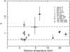Fig. 1 Thermal Comptonization index α for sources in different spectral states as a function of the electron temperature kTe. Reference papers: Cyg X–2, Farinelli et al. (2009); Sco X–1, GX 17+2, GX 340+0 and GX 3+1, Farinelli et al. (2008); GX 354–0, Di Salvo et al. (2000b); GX 349+2, Di Salvo et al. (2001), X 1658–298, Oosterbroek et al. (2001); GS 1826–238, Cocchi et al. (2010); 1E 1724–3045, Barret et al. (2000).

In Fig. 1 we report the measured values of α for this sample of sources as a function of the electron temperature kT_e. This parameter can indeed considered to be a good tracer of the source spectral state because kT_e decreases when sources move from the hard to soft state as a result of a more efficient electron cooling by the enhanced seed photon supply. Moreover, the electron temperature kT_e is a directly measurable quantity because it is related to the cut-off energy of the spectrum, and it has the advantage of being distance-independent. On the other hand, the instrumental energy-band coverage and accumulation time can play some role in biasing the measured index value. For instance, Falanga et al. (2006) performed a systematic analysis of GX 354–0 as a function of its position on the hardness-intensity diagram when the source moved from the hard to soft state. The authors fitted the 3–100 keV spectrum with a DBB+Comptt model using the slab geometry. We computed the derived α-values from their best-fit parameters, but the trend was not monotonic, covering the range α ~1–3 and reflecting a behaviour of the kT_e − τ₀ parameters (decreasing of kT_e was not followed by increasing of τ₀, as expected). It is not clear whether this was because of the lack of data below 3 keV, which is necessary to constrain the seed photon temperature, or because of the accumulation time. Thus we prefer to skip these measurements. Note also that Oosterbroek et al. (2001) performed a BeppoSAX analysis of GX 3+1 and Ser X–1, both sources characterized by typical soft state spectra, fitting them with a DBB+Comptt model, but they did not specify which geometry (sphere or slab) was assumed. We found ${\mathit{\alpha }}_{\mathrm{sph}}\mathrm{=}\mathrm{2.4}{\mathrm{4}}_{-0.59}^{\mathrm{+}\mathrm{0.89}}$ and ${\mathit{\alpha }}_{\mathrm{sl}}\mathrm{=}\mathrm{0.8}{\mathrm{7}}_{-0.25}^{\mathrm{+}\mathrm{0.42}}$ for GX 3+1, ${\mathit{\alpha }}_{\mathrm{sph}}\mathrm{=}\mathrm{1.4}{\mathrm{1}}_{-0.34}^{\mathrm{+}\mathrm{0.52}}$ and ${\mathit{\alpha }}_{\mathrm{sl}}\mathrm{=}\mathrm{0.4}{\mathrm{5}}_{-0.12}^{\mathrm{+}\mathrm{0.20}}$ for Ser X–1, respectively. Looking at Fig. 1 we note that for all analyzed sources the spectral index α lies in a belt around 1 ± 0.2, apart for the case of GX 354–0 where α ~1.6. We give a possible interpretation of these observational results in the discussion.

3. A model of the Comptonization region for a neutron star

The determination of the spectral index α obtained from Comptonization of seed photons in a bounded medium has been faced for a long time. The emerging radiation spectrum depends on several parameters such as the geometry of the plasma (e.g., slab or sphere), the electron temperature and optical depth, and the space distribution of the seed photons inside the medium. Sunyaev & Titarchuk (1980) report the value α obtained from the solution of the stationary radiative transfer equation in the non-relativistic case (Fokker-Planck approximation) obtained as a convolution of the time-dependent equation with the time-escape probability distribution for seed photons distributed according to the first eigenfunction of the space operator. Later T94, Hua & Titarchuk (1995), and TL95 extended the results to the sub-relativistic case considering both slab and spherical geometry.

In order to understand what happens in NS LMXBs sources, one has to consider the hydrodynamical conditions in the region between the accretion disk and the NS surface. We will refer to this region as the transition layer (TL), often also called boundary layer or corona. Actually, the production of a strong TC bump in the persistent X-ray spectra of NS LMXBs is thought to originate in this TL, namely the region where matter deviates from its Keplerian angular velocity in order to match that of the slowly spinning NS. The radiative and hydrodynamical configuration of the TL is mostly dictated by the Reynolds number γ (Titarchuk et al. 1998; Titarchuk & Osherovich 1999), which is proportional to the mass-accretion rate and is eventually the inverse of the viscosity parameter of the Shakura-Sunyaev disk. In particular, γ determines the radial extension of the TL and in turn, from the mass-accretion rate, its optical depth. We point out that the determination of the vertical height-scale of the TL is a very complicated problem, because it requires a complete 3D magneto-hydrodynamical treatment. Using the slim disk (thus vertical-averaged) equations for determining the radial hydrodynamical structure of the TL may indeed be an issue (e.g., Popham & Sunyaev 2001).

The enhanced radiation and thermal pressure because of higher electron temperature are expected to increase the vertical height-scale of the TL with H_tl ≈ R_ns. Moreover, the solution of the angular momentum for Reynolds number γ ≲ 5–10 gives a TL radial extension ΔR_tl ≲ 0.5   R_ns. With these characteristic length-scales, it seems more plausible to approximate the TL geometry to a slab whose normal is directed along the disk plane. We emphasize that Haardt & Maraschi (1993, hereafter HM93) determined the theoretical Comptonization index α considering a two-phase model for accretion disks in AGN, in which a hot corona is surrounding and enclosing the underlying cold accretion disk. The model can in principle be applied also to the case of solar-mass BH sources. The authors assume that the corona and the disk are two slabs at significantly different temperatures and are put in contact with each other. They concentrated on the case of high temperature (kT_e ≳ 50 keV) and low optical depth (τ₀ < 1) for the corona, so that the diffusion approximation cannot hold, which is different from what we are considering. One of the consequences of the high-temperature treatment is that electron scattering is anisotropic with a significant fraction of the power back-irradiating the disk. In the HM93 model, the inner boundary condition of the hot corona is the disk cool surface (with kT_bb < 5 eV) with energy-dependent albedo. Note also that in their geometry, 100% of the disk flux is intercepted and reprocessed by the top plasma. In the geometry considered here on the other hand, it is possible that part of the disk emission directly escapes the system, while a fraction of its flux is intercepted by the TL. We are actually interested here on this portion of the intercepted disk flux (see next section).

Because of these differences between the two models, a direct comparison of the derived theoretical results is not straightforward. The reader can refer to the paper of HM93 for further details in order to better understand the differences of our respective approaches.

3.1. Energy release in the neutron star transition layer

The energy balance in the TL is dictated by Coulomb collisions with protons (gravitational energy release), while inverse Compton and free-free emission are the main cooling channels (see a formulation of this problem in the pioneer work by Zel’dovich & Shakura 1969). However, for the characteristic electron temperature (3 keV  ≲  kT_e ≲ 30 keV) and density values (≲10^-5 g cm^-3) of these regions for NS LMXBs, Compton cooling dominates over free-free emission, and the relation between the energy flux per unit surface area of the corona Q_cor, the radiation energy density ε(τ), and electron temperature T_e is given by (see also Titarchuk et al. 1998) $\frac{{\mathit{Q}}_{\mathrm{cor}}}{{\mathit{\tau }}_{\mathrm{0}}}\mathrm{\approx }\mathrm{20.2}\mathit{\epsilon }\mathrm{\left(}\mathit{\tau }\mathrm{\right)}{\mathit{T}}_{\mathrm{e}}\mathrm{\left(}\mathit{\tau }\mathrm{\right)}\mathit{,}$(3)where τ₀ is the characteristic optical depth of the TL.

The distribution ε(τ) is obtained as a solution of the diffusion equation $\frac{{\mathrm{d}}^{\mathrm{2}}\mathit{\epsilon }}{\mathrm{d}{\mathit{\tau }}^{\mathrm{2}}}\mathrm{=}\mathrm{-}\frac{\mathrm{3}{\mathit{Q}}_{\mathrm{tot}}}{\mathit{c}{\mathit{\tau }}_{\mathrm{0}}}\mathit{,}$(4)where now Q_tot = Q_cor + Q_disk is the sum of the corona (TL) and intercepted disk fluxes, respectively. The two boundary conditions for Eq. (4) are written as $\frac{\mathrm{d}\mathit{\epsilon }}{\mathrm{d}\mathit{\tau }}{\mathrm{|}}_{\mathit{\tau }\mathrm{=}{\mathit{\tau }}_{\mathrm{0}}}\mathrm{=}\mathrm{0}\mathit{,}$(5)$\frac{\mathrm{d}\mathit{\epsilon }}{\mathrm{d}\mathit{\tau }}\mathrm{-}\frac{\mathrm{3}}{\mathrm{2}}\mathit{\epsilon }{\mathrm{|}}_{\mathit{\tau }\mathrm{=}\mathrm{0}}\mathrm{=}\mathrm{0}\mathit{,}$(6)which represent the case of albedo A = 1 at the NS surface (τ = τ₀) and no diffusion emission falling from outside onto the outer corona boundary (τ = 0). The condition for A = 1 arises from the well-established observational result of NS temperature kT_bb ~1 keV, which implies a ionized NS atmosphere. This is different from the case considered by HM93, where the cool disk temperature (<5 eV) gives rise to an energy-dependent albedo with photoelectric absorption for impinging photons with energy  ≲10 keV. Another important consideration to keep in mind is that Eq. (4) is to be considered frequency-integrated. This means that we are not dealing with the specific (energy-dependent) shape of the reflected spectrum from the NS surface, but we are considering the total energy density. The solution for ε(τ) is then given by $\mathit{\epsilon }\mathrm{\left(}\mathit{\tau }\mathrm{\right)}\mathrm{=}\frac{\mathrm{2}{\mathit{Q}}_{\mathrm{tot}}}{\mathit{c}}\left[\mathrm{1}\mathrm{+}\frac{\mathrm{3}}{\mathrm{2}}{\mathit{\tau }}_{\mathrm{0}}\left(\frac{\mathit{\tau }}{{\mathit{\tau }}_{\mathrm{0}}}\mathrm{-}\frac{{\mathit{\tau }}^{\mathrm{2}}}{\mathrm{2}{\mathit{\tau }}_{\mathrm{0}}^{\mathrm{2}}}\right)\right]\mathrm{·}$(7)Note that dε/dτ > 0 for τ < τ₀, and as F_rad ∝ dε/dτ for NS sources the radiative force always plays against gravity, unlike for BH sources.

Moreover the spectra of NS sources both in the soft and hard state can be adequately fitted by single-temperature Comptonization models (e.g., Falanga et al. 2006; Paizis et al. 2006; Farinelli et al. 2007; Cocchi et al. 2010). This observational fact demonstrates that an assumption of isothermal plasma in the TL can be applicable to X-ray data analysis from NS binaries. The question is how one can estimate this average temperature of the TL which is actually established by photon scattering and cooling processes.

In order to determine this average plasma temperature T_e one should estimate the mean energy density in the TL as $\mathrm{⟨}\mathit{\epsilon }\mathrm{\left(}\mathit{\tau }\mathrm{\right)}\mathrm{⟩}\mathrm{=}\frac{\mathrm{1}}{{\mathit{\tau }}_{\mathrm{0}}}{\mathrm{\int }}_{\mathrm{0}}^{{\mathit{\tau }}_{\mathrm{0}}}\mathit{\epsilon }\mathrm{\left(}\mathit{\tau }\mathrm{\right)}\mathrm{d}\mathit{\tau }\mathrm{=}\frac{{\mathit{Q}}_{\mathrm{tot}}}{\mathit{c}}\mathrm{(}\mathrm{2}\mathrm{+}{\mathit{\tau }}_{\mathrm{0}}\mathrm{)}\mathit{.}$(8)Note the similarity between Eqs. (3) and (8) in our paper and Eq. (13) in Bisnovatyi-Kogan et al. (1980), who studied the radiation emission due to gas accretion onto a NS. If we now substitute the result of Eq. (8) into Eq. (3), after a bit of straightforward algebra we obtain $\frac{\mathit{k}{\mathit{T}}_{\mathrm{e}}{\mathit{\tau }}_{\mathrm{0}}\mathrm{(}\mathrm{2}\mathrm{+}{\mathit{\tau }}_{\mathrm{0}}\mathrm{)}}{{\mathit{m}}_{\mathrm{e}}{\mathit{c}}^{\mathrm{2}}}\mathrm{=}\frac{\mathrm{0.25}}{\mathrm{1}\mathrm{+}{\mathit{Q}}_{\mathrm{disk}}\mathit{/}{\mathit{Q}}_{\mathrm{cor}}}\mathrm{·}$(9)Keeping in mind the definition of the Comptonization parameter Y ≈ AN_sc (Rybicki & Ligthman 1989), where A ~ 4kT_e/m_ec² and ${\mathit{N}}_{\mathrm{sc}}\mathrm{~}\mathrm{Max}\mathrm{\left(}{\mathit{\tau }}_{\mathrm{0}}\mathit{,}{\mathit{\tau }}_{\mathrm{0}}^{\mathrm{2}}\mathrm{\right)}$ are the average photon energy gain per scattering and average number of scatterings, respectively, we can rewrite Eq. (9) as $\mathit{Y}\mathrm{~}\frac{\mathrm{1}}{\mathrm{1}\mathrm{+}{\mathit{Q}}_{\mathrm{disk}}\mathit{/}{\mathit{Q}}_{\mathrm{cor}}}\mathrm{·}$(10)Equation (10) is one of the main points of our theoretical model and shows that in the diffusion approximation the Comptonization parameter, which determines the spectral index, is just a function of the corona and disk-cooling fluxes.

3.2. Radiative transfer formalism for spectral index determination

As we have shown in Sect. 2.1, the observed spectral index α of most NS LMXBs undergoes small variation around 1, namely α = 1 ± 0.2 when the electron temperature of the Compton cloud varies from about 2.5 to 25 keV (see Fig. 1). Thus we propose here a model for the spectral formation in the TL (corona) that can explain the stability of α if the flux from the disk intercepted by the corona is much less than that released in the corona itself. Namely we show that α ≈ 1 + O(Q_disk/Q_cor).

As already pointed out in standard works (Sunyaev & Titarchuk 1980, 1985, hereafter ST85, T94), spectral formation in plasma clouds of finite dimensions (bounded medium) is related to the distribution law of the number of scatterings that seed photons experience before escaping. If u_av denotes the average number of photon scatterings and the dimensionless scattering number is u = N_eσ_Tct, then the distribution law for u ≫ u_av is given by (see ST85) $\mathit{P}\mathrm{\left(}\mathit{u}\mathrm{\right)}\mathrm{=}\mathit{A}\mathrm{\left(}{\mathit{u}}_{\mathrm{av}}\mathit{,}{\mathit{\tau }}_{\mathrm{0}}\mathrm{\right)}{\mathrm{e}}^{\mathrm{-}\mathit{\beta u}}\mathit{.}$(11)For a diffusion regime when τ₀ ≳ 1.5, we get $\mathit{\beta }\mathrm{=}{\mathit{\lambda }}_{\mathrm{1}}^{\mathrm{2}}\mathit{/}\mathrm{3}$, where λ₁ is the first eigenvalue of the diffusion space operator. As reported in ST85, the eigenvalue problem for photon diffusion in a slab with total optical depth 2τ₀ is derived from solution of the differential equation for the zero-moment intensity $\frac{{\mathrm{d}}^{\mathrm{2}}\mathit{J}}{\mathrm{d}{\mathit{\tau }}^{\mathrm{2}}}\mathrm{+}{\mathit{\lambda }}^{\mathrm{2}}\mathit{J}\mathrm{=}\mathrm{0}\mathit{,}$(12)with absorption boundary conditions dJ/dτ−(3/2)J = 0 and dJ/dτ + (3/2)J = 0, for τ = 0 and τ = 2τ₀, respectively. This leads to the trascendental equation for the eigenvalue λ_n, n = 1,2,3... $\tan \mathrm{\left(}{\mathit{\lambda }}_{\mathrm{n}}{\mathit{\tau }}_{\mathrm{0}}\mathrm{\right)}\mathrm{=}\frac{\mathrm{2}}{\mathrm{3}{\mathit{\lambda }}_{\mathrm{n}}}\mathit{,}$(13)which has the solution for τ₀ ≫ 1 and n = 1 ${\mathit{\lambda }}_{\mathrm{1}}\mathrm{=}\frac{\mathit{\pi }}{\mathrm{2}\mathrm{(}{\mathit{\tau }}_{\mathrm{0}}\mathrm{+}\mathrm{2}\mathit{/}\mathrm{3}\mathrm{)}}\mathrm{·}$(14)The same result for λ₁ is obtained by solving Eq. (12) for a slab with total optical depth τ₀ but with reflection condition dJ/dτ = 0 at τ = τ₀. This is not surprising because this condition is actually met at the center of a symmetric slab with total optical depth 2τ₀ and 0 ≤ τ ≤ 2τ₀. Thus, the same mathematical result is obtained for two different geometrical configurations. In the first case (symmetric slab with total optical depth 2τ₀) it represents, e.g., an accretion disk (ST85 treatment), in our present case we are dealing with a boundary layer with total optical depth τ₀, whose asymmetry is due to the presence of a reflector (NS surface) at one of the two boundaries. In both cases one obtains $\mathit{\beta }\mathrm{=}\frac{{\mathit{\pi }}^{\mathrm{2}}}{\mathrm{12}\mathrm{(}{\mathit{\tau }}_{\mathrm{0}}\mathrm{+}\mathrm{2}\mathit{/}\mathrm{3}{\mathrm{)}}^{\mathrm{2}}}\mathrm{·}$(15)Generalizing to the case of arbitrary optical depth τ₀, the diffusion operator L_diff = (1/3)d²J/dτ² is replaced by the radiative transfer operator L_τ applied to J(τ) (see ST85 and TL95), which for disk geometry is ${\mathit{L}}_{\mathit{\tau }}\mathit{J}\mathrm{=}\frac{\mathrm{1}}{\mathrm{2}}{\mathrm{\int }}_{\mathrm{0}}^{\mathrm{2}{\mathit{\tau }}_{\mathrm{0}}}\mathit{J}\mathrm{\left(}{\mathit{\tau }}^{\mathrm{\prime }}\mathrm{\right)}{\mathit{E}}_{\mathrm{1}}\mathrm{\left(}\mathrm{\right|}\mathit{\tau }\mathrm{-}{\mathit{\tau }}^{\mathrm{\prime }}\mathrm{\left|}\mathrm{\right)}\mathrm{d}{\mathit{\tau }}^{\mathrm{\prime }}\mathrm{-}\mathit{J,}$(16)where E₁(z) is the exponential integral of the first order. In this case, the derived value for β is (T94, TL95) $\mathit{\beta }\mathrm{=}\frac{{\mathit{\pi }}^{\mathrm{2}}}{\mathrm{12}\mathrm{(}{\mathit{\tau }}_{\mathrm{0}}\mathrm{+}\mathrm{2}\mathit{/}\mathrm{3}{\mathrm{)}}^{\mathrm{2}}}\mathrm{(}\mathrm{1}\mathrm{-}{\mathrm{e}}^{\mathrm{-}\mathrm{1.35}{\mathit{\tau }}_{\mathrm{0}}}\mathrm{)}\mathrm{+}\mathrm{0.45}{\mathrm{e}}^{\mathrm{-}\mathrm{3.7}{\mathit{\tau }}_{\mathrm{0}}}\ln \frac{\mathrm{10}}{\mathrm{3}{\mathit{\tau }}_{\mathrm{0}}}\mathrm{·}$(17)Now having in mind Eq. (9), we introduce the parameter ${\mathit{\beta }}_{\mathrm{diff}}\mathrm{=}\frac{\mathrm{1}}{{\mathit{\tau }}_{\mathrm{0}}\mathrm{(}\mathrm{2}\mathrm{+}{\mathit{\tau }}_{\mathrm{0}}\mathrm{)}}\mathit{,}$(18)and in Fig. 2 we show the values of β for the cases reported in Eqs. (15), (17), and (18) as a function of optical depth τ₀. It is possible to see that actually for τ₀ ≳ 1.5 all values of β are practically close each other, but they deviate for τ₀ ≲ 1. For example their difference is about 30% for τ₀ = 1.

Using the definition of α (see Eq. (2)), where β is replaced by β_diff (Eq. (18)), and Eq. (9), we obtain the diffusion spectral index as ${\mathit{\alpha }}_{\mathrm{diff}}\mathrm{=}\mathrm{-}\frac{\mathrm{3}}{\mathrm{2}}\mathrm{+}\sqrt{\frac{\mathrm{9}}{\mathrm{4}}\mathrm{+}\frac{\mathrm{1}\mathrm{+}{\mathit{Q}}_{\mathrm{disk}}\mathit{/}{\mathit{Q}}_{\mathrm{cor}}}{\mathrm{0.25}}}\mathit{,}$(19)or α_diff ≈ 1 + 0.8   Q_disk/Q_cor for Q_disk/Q_cor ≪ 1.

Thus, as it follows from Eq. (19), in the diffusion regime the TC spectral index can be expressed in terms of Q_disk/Q_cor (the intercepted disk over corona fluxes), instead of TL electron temperature kT_e and optical depth τ₀ (see Eqs. (2) and (15)). In Fig. 3 we present a plot of α_diff as a function of Q_disk/Q_cor, which shows that it ranges from 1 to 1.6 as Q_disk/Q_cor increases from 0 to 1. One can see that the observable value of α ~ 1 takes place if the energy release in the disk is much less than in TL, namely if Q_disk/Q_cor ≪ 1.

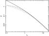Fig. 2 Values of the β-parameter as a function of the optical depth τ0. The solid, dashed, and dotted lines correspond to definition of β given in Eqs. (15), (17), and (18), respectively.

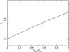Fig. 3 Theoretical thermal Comptonization index α as a function of the ratio Qdisk/Qcor according to Eq. (19).

4. Results and discussion

We compared observational data of a sample of NS LMXB sources (Fig. 1) with the theoretical results that follow from the radiative transfer model in the diffusion approximation. The data show that independently of the source spectral state, which we have parametrized through the measured TL electron temperature kT_e, the spectral index α = 1 ± 0.2. We derived an estimate of the energy index α for TC spectra in NS LMXBs using an equation for the diffusion approximation in a slab geometry with reflection boundary condition at the NS surface, which is valid for optical depth τ₀ ≳ 1.5. In particular, we find that in this approximation it is possible to express the value of α as a function of the ratio of the flux from the accretion disk intercepted by the corona (TL) and the energy release in the corona itself (see Eq. (19)). The agreement of the model with the data is reached when the condition Q_disk/Q_cor ≪ 1 holds (see Fig. 3).

This behavior of the spectral index α actually has important consequences on putting constraints in the accretion geometry of NS LMXBs. Indeed, as already pointed-out in the introduction, the broadband persistent X-ray spectra of these sources are usually fitted by a two-component model consisting of BB-like emission plus a strong TC bump. Both the cases for which the BB temperature (kT_bb) is lower or higher than that of the seed photons of the TC bump (kT_s) provide equally acceptable fits. In the first case (kT_bb < kT_s), the origin of the direct BB component is attributed to the accretion disk, in the second case (kT_bb > kT_s) to the NS surface. This dichotomy in the spectral analysis has not been overcome for a long time. Some help in this direction has come with the discovery of the transient X-ray tails in some of the brightest sources (see references in the introduction): if the origin of the hard PL-like X-ray emission is attributed to a combined thermal plus bulk (converging flow) effect in the innermost part of the TL close to the NS surface, it becomes natural to suggest that the observed direct BB photon spectrum mostly originates in the TL/NS surface region, providing the seed photons for bulk Comptonization (see Fig. 1 in Farinelli et al. 2007).

The theoretical results derived here strengthen this scenario. When computing the total energetic spectral budget of the sources in the 0.1–40 keV (where most of the emission is produced), the dominating TC bump carries out more than 70% of the source luminosity, and the remaining part is due to the direct BB component. If this BB originates close to the NS surface, it is evident that the disk contribution to the X-ray luminosity is very small. Given that Q_disk in Eq. (19) represents the flux from the accretion disk intercepted by the corona and thus is smaller or at most equal to the directly emitted part, this eventually leads to α ~ 1. In this framework, we can make some considerations about the higher value of α (~1.6) measured for GX 354–0 (see Fig. 1). Di Salvo et al. (2000b) fitted the broadband spectrum of the source with a BB+Comptt model with kT_bb < kT_s, a modelization corresponding to the case where a significantly higher fraction of the X-ray luminosity comes from the accretion disk. This would turn of course into an enhanced value of Q_disk, and looking at Fig. 3 it is evident that increasing Q_disk/Q_cor corresponds to increasing α. Actually, it would be interesting to see what does happen by fitting the BeppoSAX spectra of GX 354–0 with the same model, but with kT_bb > kT_s. Note also in Fig. 1 that for 1E 1724–3045 and two spectral states of GS 1826–238, α ~ 1 with electron temperature kT_e ≳ 20 keV. With Eq. (9) and the best-fit values of kT_e reported for the two sources, with Q_disk/Q_cor ~ 0, we obtain τ₀ ~ 1.3 for 1E 1724–3045 and τ₀ ~ 1.6–1.7 for GS 1826–238, respectively. These values of the optical depth allow us to actually deal with the diffusion approximation within a degree of accuracy that is still satisfactory, as can be seen from Fig. 2. Moreover, for a slab with optical depth τ₀ and inner reflection boundary condition, photons that are back-scattered from the reflecting surface before escaping experience an optical depth  ~2τ₀, which further enhances the diffusion approximation validity.

The other issue to point out is that the lower limit on α (for the extreme case Q_disk/Q_cor = 0) derived by our model is 1, while there is a handful of sources for which 0.8 < α < 1. Different reasons can lead to this result. First of all, it is well known that multi-component modeling of X-ray spectra may have some influence in the determination of the best-fit parameters. In particular, in the energy band where TC dominates (≲ 30 keV), Gaussian emission lines around 6.4–6.7 keV are often observed, and the inclusion of narrow-feature component in the model can affect the continuum parameters. Additional biases can come from the energy-band coverage (in particular when using RXTE data, which start from about 3 keV) and uncertainties in the calibration of the instrumental effective area, which may play some role in particular for spectra that are far away from being powerlaw-like.

In terms of theoretical predictions, our analytical model is intended to provide a description of the observed stability of the spectral index but may of course have some limitations, in particular the energy-independent treatment of the radiation field and the simple slab approximation for the TL geometry. Yet, if it is possible that the vertical height-scale H_tl of the TL is higher than its radial extension, it is also likely that there is some dependence of H_tl on the radial distance from the NS surface. Moreover, in the pure plane-parallel geometry photons are allowed to escape only through the surface of the slab, while here the slab has limited extension and photons presumably can escape also from its lateral walls.

5. Conclusions

We reported results on the value of the thermal Comptonization spectral index α for a sample of NS LMXB sources in different spectral cases and found that apart from GX 354–0 it lies in a belt around 1 ± 0.2. We proposed a simple theoretical model using the diffusion approximation where α is found to be a function only of the ratio of the disk and corona fluxes. In particular, the condition Q_disk/Q_cor ≪ 1 leads to α ~1, which is consistent with observations. We are hopeful that our work will encourage to significantly extend the sample of observed sources using archival data and observations from present and future missions, in particular using as broad as possible energy band, especially below 3 keV in order to avoid biases in the spectral results. We also claim that our model can be helpful in solving the dichotomy related to the fact that equally good fits are obtained for the cases where the observed direct BB component has a temperature higher or lower than that of the seed photons subjected to thermal Comptonization.

Acknowledgments

The authors are grateful to the referee whose suggestions greatly improved the quality of the paper with respect to the first version. This

work was supported by grant from Italian PRIN-INAF 2007, “Bulk motion Comptonization models in X-ray Binaries: from phenomenology to physics”, PI M. Cocchi.

References

All Figures

Fig. 1 Thermal Comptonization index α for sources in different spectral states as a function of the electron temperature kTe. Reference papers: Cyg X–2, Farinelli et al. (2009); Sco X–1, GX 17+2, GX 340+0 and GX 3+1, Farinelli et al. (2008); GX 354–0, Di Salvo et al. (2000b); GX 349+2, Di Salvo et al. (2001), X 1658–298, Oosterbroek et al. (2001); GS 1826–238, Cocchi et al. (2010); 1E 1724–3045, Barret et al. (2000).

In the text

	Fig. 2 Values of the β-parameter as a function of the optical depth τ0. The solid, dashed, and dotted lines correspond to definition of β given in Eqs. (15), (17), and (18), respectively.
In the text

	Fig. 3 Theoretical thermal Comptonization index α as a function of the ratio Qdisk/Qcor according to Eq. (19).
In the text

References

- Barret, D., Olive, J. F., Boirin, L., et al. 2000, ApJ, 533, 329 [NASA ADS] [CrossRef] [Google Scholar]
- Bisnovatyi-Kogan, G. S., Khlopov, M. Y., Chechetkin, V. M., & Eramzhyan, R. A. 1980, SvA, 24, 716 [Google Scholar]
- Cocchi, M., Farinelli, R., Paizis, A., & Titarchuk, L. 2010, A&A, 509, 2 [Google Scholar]
- D’Amico, F., Heindl, W. A., Rothschild, R. E., et al. 2001, ApJ, 547, L147 [NASA ADS] [CrossRef] [Google Scholar]
- Di Salvo, T., Stella, L., Robba, N. R., et al. 2000a, 554, L119 [Google Scholar]
- Di Salvo, T., Iaria, R., Burderi, L., & Robba, N. R. 2000b, ApJ, 542, 1034 [NASA ADS] [CrossRef] [Google Scholar]
- Di Salvo, T., Robba, N. R., Iaria, R., et al. 2001, ApJ, 554, 49 [NASA ADS] [CrossRef] [Google Scholar]
- Di Salvo, T., Farinelli, R., Burderi, L., et al. 2002, A&A, 386, 535 [NASA ADS] [CrossRef] [EDP Sciences] [Google Scholar]
- Di Salvo, T., Goldoni, P., Stella, L., et al. 2006, ApJ, 649, L91 [NASA ADS] [CrossRef] [Google Scholar]
- Falanga, M., Godtz, D., Goldoni, P., et al. 2006, A&A, 458, 21 [NASA ADS] [CrossRef] [EDP Sciences] [Google Scholar]
- Farinelli, R., Titarchuk, L., & Frontera, F. 2007, ApJ, 662, 1167 [NASA ADS] [CrossRef] [Google Scholar]
- Farinelli, R., Titarchuk, L., Paizis, A., & Frontera, F. 2008, ApJ, 680, 602 (F08) [NASA ADS] [CrossRef] [Google Scholar]
- Farinelli, R., Paizis, A., Landi, R., & Titarchuk, L. 2009, A&A, 498, 509 [NASA ADS] [CrossRef] [EDP Sciences] [Google Scholar]
- Gierliński, M., & Done, C. 2002, MNRAS, 337, 1373 [Google Scholar]
- Haardt, F., & Maraschi, L. 1993, ApJ, 413, 50 (HM93) [Google Scholar]
- Hua, X.-M., & Titarchuk, L. 1995, ApJ, 449, 188 [NASA ADS] [CrossRef] [Google Scholar]
- Laurent, P., & Titarchuk, L. 1999, ApJ, 511, 289 [NASA ADS] [CrossRef] [Google Scholar]
- Lavagetto, G., Iaria, R., di Salvo, T., et al. 2004, Nucl. Phys. B, Proc. Suppl., 132, 616 [NASA ADS] [CrossRef] [Google Scholar]
- Mitsuda, K., Inoue, H., Koyama, K., et al. 1984, PASJ, 36, 741 [NASA ADS] [Google Scholar]
- Mitsuda, K., Inoue, H., Nakamura, N., & Tanaka, Y. 1989, PASJ, 41, 97 [NASA ADS] [Google Scholar]
- Montanari, E., Titarchuk, L., & Frontera, F. 2009, ApJ, 692, 1597 [NASA ADS] [CrossRef] [Google Scholar]
- Oosterbroek, T., Parmar, A. N., Sidoli, L., in’t Zand, J. J. M., & Heise, J. 2001, A&A, 370, 532 [NASA ADS] [CrossRef] [EDP Sciences] [Google Scholar]
- Paizis, A., Ebisawa, K., Tikkanen, T., et al. 2005, A&A, 435, 599 [CrossRef] [EDP Sciences] [Google Scholar]
- Paizis, A., Farinelli, R., Titarchuk, L., et al. 2006, A&A, 459, 187 [NASA ADS] [CrossRef] [EDP Sciences] [Google Scholar]
- Popham, R., & Sunyaev, R. A. 2001, ApJ, 547, 355 [NASA ADS] [CrossRef] [Google Scholar]
- Rybicki, G. B., & Lightman, A. P. 1979, Radiat. Processes Astrophys. (New York: Wiley) [Google Scholar]
- Sunyaev, R. A., & Titarchuk, L. 1980, A&A, 86, 121 [NASA ADS] [Google Scholar]
- Sunyaev, R. A., & Titarchuk, L. 1985, A&A, 143, 374 [NASA ADS] [Google Scholar]
- Shaposhnikov, N., & Titarchuk, L. 2009, ApJ, 699, 453 [NASA ADS] [CrossRef] [Google Scholar]
- Titarchuk, L. 1994, ApJ, 434, 570 (T94) [NASA ADS] [CrossRef] [Google Scholar]
- Titarchuk, L., & Lyubarskij, Y. 1995, ApJ, 450, 876 (TL95) [NASA ADS] [CrossRef] [Google Scholar]
- Titarchuk, L., & Osherovich, V. 1999, ApJ, 518, L95 [NASA ADS] [CrossRef] [Google Scholar]
- Titarchuk, L., & Fiorito, R. 2004, ApJ, 612, 988 [NASA ADS] [CrossRef] [Google Scholar]
- Titarchuk, L., & Shaposhnikov, N. 2005, ApJ, 626, 298 [NASA ADS] [CrossRef] [Google Scholar]
- Titarchuk, L., & Seifina, E. 2009, ApJ, 706, 1463 [NASA ADS] [CrossRef] [Google Scholar]
- Titarchuk, L., Mastichiadis, A., & Kylafis, N. D. 1997, ApJ, 487, 831 [NASA ADS] [Google Scholar]
- Titarchuk, L., Lapidus, J., & Muslimov, A. 1998, ApJ, 499, 315 [NASA ADS] [CrossRef] [Google Scholar]
- White, N. E., Peacock, A., Hasinger, G., et al. 1986, MNRAS, 218, 129 [NASA ADS] [CrossRef] [Google Scholar]
- White, N. E., Stella, L., & Parmar, A. 1988, ApJ, 324, 363 [NASA ADS] [CrossRef] [Google Scholar]
- Zel’dovich, Ya. B., & Shakura, N. I. 1969, Sov. Astron., 13, 175 [NASA ADS] [Google Scholar]