| Issue |
A&A
Volume 525, January 2011
|
|
|---|---|---|
| Article Number | A26 | |
| Number of page(s) | 9 | |
| Section | Stellar structure and evolution | |
| DOI | https://doi.org/10.1051/0004-6361/200913895 | |
| Published online | 29 November 2010 | |
The mass ratio and initial mass functions in spectroscopic binaries
1
Departamento de AstronomiaUniversidade Federal do Rio Grande do
Sul,
Av. Bento Gonçalves 9 500,,
91 501-970
Porto Alegre,
Brazil
e-mail: This email address is being protected from spambots. You need JavaScript enabled to view it.
2
Observatório do Valongo, Universidade Federal do Rio de Janeiro,
Ladeira Pedro Antônio 43,
20
080-090
Rio de Janeiro,
Brazil
Received:
17
December
2009
Accepted:
8
September
2010
Abstract
Context. Spectroscopic binaries are important in studies of binary star-formation, since original information linked to the forming stars, such as the mass ratio, can be kept in the system and observationally retrieved.
Aims. We aim to derive the more probable mass ratio distributions, to test a possible Initial Mass Functions acting on the formation of spectroscopic binaries, and to derive the value of q0, the minimal mass ratio for which both binary components are simultaneously in the main sequence.
Methods. The sample has 249 systems, selected from the Ninth Catalogue of Spectroscopic Binaries, with selection criteria that include only those systems with periods longer than four days and magnitudes brighter than mV = 7.0, and main-sequence primaries, to avoid mass exchange. Monte Carlo simulations of observational parameters were performed. We performed simulations by comparing an observational quantity, Yobs, equal to f(m)/m1, where f(m) is the mass function, to theoretical Yth, which is a function of the system inclination (assumed to be random), and of the mass ratio q = m2/m1. We considered a minimal mass ratio q0, which is the limiting condition, to ensure that both components are simultaneously on main sequence, avoiding evolutionary effects leading to mass exchange and loss of information on the original masses. Calculations were done using several q0 values. The form of the distribution of mass ratios was studied by simulations of Y, involving several functions, with slopes which are increasing, decreasing, constant, or bimodal. Other simulations were done by the generation of stars following several initial mass function laws. We combined pairs of stars generated from different IMFs, assuming that binaries arise from the pairing of stars simultaneously formed. In this case, several values of q0 were also used in the input equations.
Results. Our results indicate that decreasing q distributions match better with observations and also that a unique IMF gives better fits to observations than a composite IMF, with a slope around 1.4, rather than the widely used 2.35 slope. Values of q0 tend to be lower than what is suggested by previous studies, which point to q0 around 0.2; all simulations suggest that q0 values as low as 0.08 produce the best fits to observations.
Key words: binaries: spectroscopic
Present address: Greenberg fellow, Leiden Observatory, University of Leiden, PO Box 9 513, 2 300 RA Leiden, The Netherlands
e-mail: This email address is being protected from spambots. You need JavaScript enabled to view it.
Present address: Centro Brasileiro de Pesquisas Físicas, Rua Dr. Xavier Sigaud 150, 22 290–180 Rio de Janeiro, Brazil
e-mail: This email address is being protected from spambots. You need JavaScript enabled to view it.
© ESO, 2010
1. Introduction
The understanding of star formation can benefit from data of binary stars, since these systems carry information which is lost when single stars form (Larson 2001). However, formation processes of binary and multiple stars are far from being completely understood. Possible processes include simultaneous condensation from a common primordial nebula, fission, and after-condensation capture. Numerical simulations involving now available high-performance computing have provided some new insights on this question (Tohline & Durisen 2001). Alternative approaches can use models describing those processes taking as a fundamental parameter the mass ratio, q = m2/m1 (m1 and m2 being the primary and second masses of the binary components), on the grounds that some values of q are only possible from certain processes, and that different physical processes can favor higher or lower values of the mass ratio. The form of the mass ratio distribution, f(q), has been the object of extensive discussion on whether f(q) decreases or increases with increasing q, if it has a bimodal behavior, or if f(q) depends on the orbital period. Model-fitting approaches have produced results in every direction. Decreasing functions, of the form q−7/3, were suggested by Jaschek & Ferrer (1972); this function has some theoretical background, because it is the original mass function of Salpeter (1955), as pointed out by Jaschek (1969). Besides, this paper by Jaschek and Ferrer introduced the parameter q0, the minimal mass ratio that ensures that both stars are simultaneously at the main sequence, thus avoiding conditions where evolutionary processes lead to mass exchange and loss of information on primordial component masses. Concerning mass ratio distributions, similar results were published more recently by Heacox (1998). However, more results have been published favoring other f(q)’s. Hogeveen (1990; 1992a,b) finds that f(q) can be a power law, either decreasing or increasing, depending on whether the sample (from Batten et al. 1978 Eighth Catalogue of Spectroscopic Binaries – SB) was formed by single-line (SBI) or double-line (SBII) systems. This calls attention to the extent to which selection effects can influence results. Increasing f(q)s, with peaks near high q’s were suggested by Lucy & Ricco (1979), among others, for close SBs; however, most studies with similar results (Garmany et al. 1980; Abt & Levy 1985; Levato et al. 1987; Fekel et al. 1988) are based on samples composed of close systems, where contact or mass exchange lead to loss of information on the original mass of the components. Bimodal distributions have been suggested by Trimble (1974), and as well by Abt & Levy (1976); finally, both qn and bimodal distributions were the results of model-fittings by Dabrowski & Beardsley (1977) and Trimble & Ostriker (1978). Also based on Batten’s Eighth Catalogue is the study by Fisher et al. (2005) concerning a sample of local field stars, which indicated a q distribution of field binaries with many q values near unity, and thus dominated by double-lined systems. The above results indicate that confusion does exist, a problem that can be approached by the use of carefully selected samples where biases are minimized. The recent release of a large database on spectroscopic binary stars has allowed more significant model-fitting tests. The choice of spectroscopic systems is convenient because of the availability of useful parameters, especially radial velocities, which in visual binaries lack the necessary accuracy and amplitude. Using a selected sample of spectroscopic binaries as a reference, the scope of this work is threefold: to look for the more probable mass ratio distributions, to test Initial Mass Functions acting during binary formation, and to derive values for the parameter q0; to reach these objectives, we performed Monte Carlo simulations involving assumptions on mass ratio distributions, on initial mass functions, and testing several q0 values.
2. Data and basic methodology
Following former compilations of spectroscopic binary observational parameters, for example, that by Batten et al. (1978), we selected the observational sample from the online version of the Ninth Catalogue of Spectroscopic Binary Orbits (Pourbaix et al. 2004), which provides information on 2385 systems. Observational biases are certainly present, and several criteria were applied to compile a sample with a bias as small as possible, as follows:
-
a)
An important bias in the Ninth Catalogue is that the percentageof eclipsing binaries is statistically increased. This happensbecause variability is easily detected, and systems with deepereclipses are even more easily discovered, because they havecomponents of similar brightness and, therefore, with highermass ratios. This bias in favor of eclipsing SBs is stronger infainter systems. To minimize this bias, the sample included onlybinaries brighter thanmV = 7.0, on the grounds that those objects belonging to the bright star catalogue (BSC) and its Supplement (Warren & Hoffleit 1987), which list systems brighter than mV = 7.0, have been extensively observed and few spectroscopic systems, if any, remain undetected.
-
b)
Mass exchange may influence the evolution of close systems, so to ensure a sample that conserves the original information of both components, the sample included only systems with periods longer than four days, corresponding to orbits with semi-major axis of about 7.4 million kilometers. This value is about 40% higher than the largest O stars in the sample, and accordingly, systems with possible contact between the components were not included in the compilation. This criterion leads to the exclusion of certain pairs of multiple systems (HD 25 204, HD 36 695, HD 71 663, HD 157 482, HD 201 433), even if these systems would have remained in the sample due to other criteria.
-
c)
Another condition imposed to avoid mass exchange was the exclusion of all systems with non-main sequence primaries. These last two criteria are complementary, producing a sample with non-interacting stars even for the eventual systems which, being formed by capture, do not have coeval components.
The final, homogeneous sample, had 249 systems, with primary spectral types distributed as follows: 29% OB, 55% AF, 16% GK. The list of stars is given in Table 2 at the end of this paper. This sample is significantly greater than those used in most of the papers cited in Sect. 1, and includes single (144 objects) and double-lined (105) systems.
A special mention has to be made concerning the paper by Fisher et al. (2005), because this paper, in a first analysis, has partially similar scopes and sources of data. However, an important objective for us was to derive values of q0, a parameter which was not approached in their paper because it is seldom studied. Approaches to the other scopes are heavily influenced by the sample used, and here, it is true that the present sample of 249 systems is smaller than that of Fisher and collaborators, which has 371 objects; these samples, however, have some important differences. The larger sample was compiled with data from Batten’s Eighth Catalogue and from private communications; it used all values of periods, thus allowing the inclusion of contact systems and evolved stars, where mass exchanges can occur, processes which modify the original mas ratios at system formation. Unfortunately, the paper by Fisher et al. (2005) does not provide the list of systems forming the sample used for their study, so a direct comparison is not possible. However, from their criteria of d ≤ 100 pc and MV ≤ 4, it can be deduced that for later stars, G and K dwarfs are excluded, because of the luminosity criterion. On the earlier side, an examination of the Bright Star Catalogue suggests that there are significant differences between Fisher’s and our sample. For example, from the BSC it is evident that the criterion for distances smaller than 100 pc only allows the inclusion, in Fisher’s sample, of about eight dwarfs of spectral type B3 or hotter, not necessarily primaries of spectroscopic binaries. On the other hand, GK dwarfs make up 16% of primaries of our sample, which besides includes 31 B3, or earlier, dwarf primaries. The same reasoning extends to all B dwarfs. Consequently, even if the exact content of Fisher’s list is not known, a clear perception arises that the ensemble of these differences is very significant and results in very different samples, for the spectral types and luminosity classes, and also for the volume of space studied.
Mass ratios can be directly derived from the radial velocities measured from SBIIs;
however, with the present number of 105 systems, they are not enough to provide reliable
information about the form of a mass ratio distribution. Besides, in doing this, the
resulting sample presents a bias towards higher mass ratios, a perception already expressed
at the modelings performed by Tout (1991). This
author, and also Hogeveen (1992a), use different
arguments to show that an inverse bias is present if only SBI systems are used. Indeed, both
cite and use a former result, summarized in Fig. 1 of Staniucha (1979). The database used to produce this result carries the biases which
are avoided in our sample. Also, given a fixed sample, the relative proportion of SBI to
SBII will change steadily in favor of SBII, as time passes and observational techniques
improve. Modeling this shifting subsamples separately would give unreliable results. So, the
question is how to avoid those biases, and at the same time, how to put the observational
information from systems with only one spectrum into a useful form. The so-called “mass
function”, f(m), is a well known expression that addresses
this problem. Not to be confused with the Initial Mass Function, the
f(m) for spectroscopic binaries is derived from Kepler’s
third law, and has been presented and used in Halbwachs (1987) or in Duquennoy & Mayor (1991)
among others. It is given by 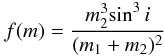 (1)with
m1 and m2 defined as above, and
i the inclination of the plane of the system with respect to the line of
sight. The mass function can also be expressed in terms of observational quantities, in the
form
(1)with
m1 and m2 defined as above, and
i the inclination of the plane of the system with respect to the line of
sight. The mass function can also be expressed in terms of observational quantities, in the
form  (2)where
k1 is the radial velocity of the primary component, in
km s-1, P is the period in days, and e is the
system’s orbital eccentricity. This allows the use of SBI in exactly the same way as for
SBII, as was pointed by Trimbe (1990), with the
advantage that only information from the primary is needed. In a lengthy analysis, and after
stating that it is impossible to determine an overall mass-ratio distribution by adding the
observed q distributions of SBI and SBII systems, Hogeveen (1992b) finally suggests that the observed
q distribution of SBII systems is compatible with the assumption that all
binary stars in the solar neighborhood have mass ratios distributed according to the
intrinsic q distribution found from SBI systems. The purpose of this study
is to perform a comparison of observational information from Eq. (2) with theoretical
predictions from Eq. (1); here, a problem arises because to use Eq. (1) one has to know
m2, a piece of information that is absent from Eq. (2).
(2)where
k1 is the radial velocity of the primary component, in
km s-1, P is the period in days, and e is the
system’s orbital eccentricity. This allows the use of SBI in exactly the same way as for
SBII, as was pointed by Trimbe (1990), with the
advantage that only information from the primary is needed. In a lengthy analysis, and after
stating that it is impossible to determine an overall mass-ratio distribution by adding the
observed q distributions of SBI and SBII systems, Hogeveen (1992b) finally suggests that the observed
q distribution of SBII systems is compatible with the assumption that all
binary stars in the solar neighborhood have mass ratios distributed according to the
intrinsic q distribution found from SBI systems. The purpose of this study
is to perform a comparison of observational information from Eq. (2) with theoretical
predictions from Eq. (1); here, a problem arises because to use Eq. (1) one has to know
m2, a piece of information that is absent from Eq. (2).
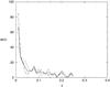 |
Fig. 1 Histogram for observed Y, from 249 spectroscopic binaries (solid line). Also shown are normalized tracings of sub-samples, for periods longer (dotted line) or shorter (dot-dashed line) than 40 days. |
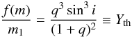 (3)and for the
observational equation
(3)and for the
observational equation 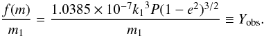 (4)The modeling of
Yth, as just defined, will be compared with observations,
expressed by Yobs. To obtain Yobs,
the masses of the primary stars are needed. With the spectral types (main sequence) of the
primaries being known for all 249 objects in the sample, the masses of the primaries can be
obtained from a spectral type-mass table, like that from Lang (1991), where missing spectral types had their masses determined by
iteration. With data on periods and eccentricity from the Ninth Catalogue, it was possible
to derive the mass function, and Yobs. The histogram for
Yobs is shown in Fig. 1.
To investigate a possible dependency of the period on the mass function, the observational
sample was divided into two groups: periods longer or shorter than 40 days, a value that
approximately divides the sample into two equal parts. The normalized traces for these
sub-samples are also shown in Fig. 1.
(4)The modeling of
Yth, as just defined, will be compared with observations,
expressed by Yobs. To obtain Yobs,
the masses of the primary stars are needed. With the spectral types (main sequence) of the
primaries being known for all 249 objects in the sample, the masses of the primaries can be
obtained from a spectral type-mass table, like that from Lang (1991), where missing spectral types had their masses determined by
iteration. With data on periods and eccentricity from the Ninth Catalogue, it was possible
to derive the mass function, and Yobs. The histogram for
Yobs is shown in Fig. 1.
To investigate a possible dependency of the period on the mass function, the observational
sample was divided into two groups: periods longer or shorter than 40 days, a value that
approximately divides the sample into two equal parts. The normalized traces for these
sub-samples are also shown in Fig. 1.
3. Simulations from mass ratio functions
The function Yth depends on the form of the distribution function of mass ratios, f(q). The modeling of Yth, which will be compared to Yobs, thus totally depends on the expression of f(q). This is done by assuming several test f(q)’s, which are each used to generate a Yth. With respect to the sini dependency in Eq. (3), inclinations of systems are supposed to be random, as widely accepted (Halbwachs 1987). The choice of test f(q)’s must cover most of the possible slopes or forms. Table 1 lists the f(q)’s used in simulations.
List of mass ratio, q distributions used in the construction of histograms for theoretical Y.
The construction of the histograms for Yth was made for each
q distribution listed in Table 1,
by generation of successive Yth values using random numbers. The
procedure is as follows: given any distribution f(q),
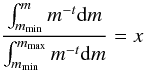
 (5)Here, x is
a random number and the q0 parameter is introduced, which is the
minimal mass ratio that ensures that both stars are simultaneously at the main sequence,
thus avoiding conditions where evolutionary processes lead to mass exchange and loss of
information on primordial component masses; in this sense, q0 is
a critical parameter for this study, and finding its value is a result in itself. It can be
determined from evolutionary lifetime models, following Iben (1964). A system in which the primary is too massive with respect to its
secondary will never have both components simultaneously in the main sequence, because by
the time the secondary arrives at the ZAMS, the primary will already have left it. The
approximate limit of q0 for coexistence as dwarfs would be
around 0.17, as suggested by Giannone & Giannuzzi (1969) and Jaschek (1969). Solving the
integrals (Eq. (5)) for each distribution leads to an expression for q that
contains both q0 and x. A similar procedure is
performed for the sine component. Values of modeled Yth
(Eq. (3)) are generated in this way and successive executions lead to the construction of
histograms, one for each adopted f(q) distribution, where
a q0 value is adopted. These modeled histograms have to be
compared to the Yobs histogram. The comparison takes into
account that the observational sample contains non-negligible noise, because it is
relatively small (249 objects), even if it is one of the largest compiled to date. So,
simulations for each f(q) were, accordingly, generated up
to 249 executions, producing histograms of Yth which have the
same size as the Yobs histogram; the histogram for
Yth has a noise similar to the
Yobs noise and, because it has the same size, allows also a
comparison on a normalized basis. Both distributions, Yobs and
Yth, are compared point-to-point for 25 partitions in the
domain of possible Y values, which go from 0 to 0.25. The modulus of the
difference within any partition k is
(5)Here, x is
a random number and the q0 parameter is introduced, which is the
minimal mass ratio that ensures that both stars are simultaneously at the main sequence,
thus avoiding conditions where evolutionary processes lead to mass exchange and loss of
information on primordial component masses; in this sense, q0 is
a critical parameter for this study, and finding its value is a result in itself. It can be
determined from evolutionary lifetime models, following Iben (1964). A system in which the primary is too massive with respect to its
secondary will never have both components simultaneously in the main sequence, because by
the time the secondary arrives at the ZAMS, the primary will already have left it. The
approximate limit of q0 for coexistence as dwarfs would be
around 0.17, as suggested by Giannone & Giannuzzi (1969) and Jaschek (1969). Solving the
integrals (Eq. (5)) for each distribution leads to an expression for q that
contains both q0 and x. A similar procedure is
performed for the sine component. Values of modeled Yth
(Eq. (3)) are generated in this way and successive executions lead to the construction of
histograms, one for each adopted f(q) distribution, where
a q0 value is adopted. These modeled histograms have to be
compared to the Yobs histogram. The comparison takes into
account that the observational sample contains non-negligible noise, because it is
relatively small (249 objects), even if it is one of the largest compiled to date. So,
simulations for each f(q) were, accordingly, generated up
to 249 executions, producing histograms of Yth which have the
same size as the Yobs histogram; the histogram for
Yth has a noise similar to the
Yobs noise and, because it has the same size, allows also a
comparison on a normalized basis. Both distributions, Yobs and
Yth, are compared point-to-point for 25 partitions in the
domain of possible Y values, which go from 0 to 0.25. The modulus of the
difference within any partition k is
 (6)and the total difference
between the histograms is
(6)and the total difference
between the histograms is  (7)This comparison is
performed repeatedly to generate a mean difference, which is given by
(7)This comparison is
performed repeatedly to generate a mean difference, which is given by
 (8)Here, N
was set to 1000, a value sufficient for the convergence of
(8)Here, N
was set to 1000, a value sufficient for the convergence of
 . This
procedure, which has made on a normalized basis, produces values of D within the
interval (0, 1), where
. This
procedure, which has made on a normalized basis, produces values of D within the
interval (0, 1), where  means a model totally different
from the observations. Values of D for selected test distributions from
Table 1 are presented in Fig. 2, which also gives information on the minimal mass
ratio, q0.
means a model totally different
from the observations. Values of D for selected test distributions from
Table 1 are presented in Fig. 2, which also gives information on the minimal mass
ratio, q0.
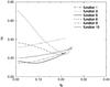 |
Fig. 2 Behavior of simulations of binary formation, compared to observations. Several mass distributions from Table 1 are shown. Distributions favoring lower mass ratios and values of q0, the minimal mass ratio around 0.08 provides the best fits. |
4. Simulations from initial mass functions
Another modeling of the observed Y was performed by creating binary
systems from the random combination, two by two, of stars generated following a formation
law: the Initial Mass Function. The expression of the IMF, since its first formulation by
Salpeter (1955), has been frequently modified. More
recently, Kennicut (1998) suggested that observations
are best fitted by a composite IMF, with a slope 1.4 for formation up to one solar mass, and
a slope 2.35 for greater masses. However, the situation can be different when star-forming
cores undergo fragmentation, a scenario studied by Goodwin & Kroupa (2005). In these cases, a binary can be formed after
additional members are ejected from the system, leading to the formation of close binaries.
This would fit the description of many spectroscopic binaries, in which case a slightly
different IMF could apply. The fragmentation process can produce stars of different masses,
the smaller ones are the first to be ejected. The two remaining masses may or may not obey a
specific, even composite IMF. To test these possibilities we performed a simulation of the
random combination of stars that are independently formed. Here, the variables are the
minimum and maximum masses possible in the star-formation processes and the IMF slopes; many
values around those suggested by Kennicut were tested. The minimal mass was set to
0.06 solar masses; the upper limit for stellar masses was set to 120 solar masses, a
conservative approach to the value suggested by Figer (2005). The generation of masses m1 and
m2 starts with the equation
 (9)where
t, the slope of the IMF is also a variable with values
t1 and t2, allowing the existence
of a composite IMF (Kennicut 1998). The generation of
m1 and m2 is subject to conditions
that, if t is t1, masses greater than a
critical value (here, one solar mass) are discarded; and if t is
t2, masses smaller than the critical value are discarded.
Here, t1 and t2 are first defined;
which one will be used comes from a random sorting; this
ti value is then used to generate
m1, and after a new
ti definition, the mass
m2 is generated. Therefore, in all systems created by this
simulation, IMFs for primaries and secondaries can be different. The same consideration for
q0 already made in Sect. 3 applies. Repeated executions are
performed, and applied in Eq. (3) together with the random sini, to produce
a histogram of simulated Yth, which can be compared to the
observations. We did this following the same procedure described in the previous section;
the number of modules of point-to-point subtractions, observational minus modeling, was also
set to be 1000. We show some results for various slopes and q0
in Fig. 3.
(9)where
t, the slope of the IMF is also a variable with values
t1 and t2, allowing the existence
of a composite IMF (Kennicut 1998). The generation of
m1 and m2 is subject to conditions
that, if t is t1, masses greater than a
critical value (here, one solar mass) are discarded; and if t is
t2, masses smaller than the critical value are discarded.
Here, t1 and t2 are first defined;
which one will be used comes from a random sorting; this
ti value is then used to generate
m1, and after a new
ti definition, the mass
m2 is generated. Therefore, in all systems created by this
simulation, IMFs for primaries and secondaries can be different. The same consideration for
q0 already made in Sect. 3 applies. Repeated executions are
performed, and applied in Eq. (3) together with the random sini, to produce
a histogram of simulated Yth, which can be compared to the
observations. We did this following the same procedure described in the previous section;
the number of modules of point-to-point subtractions, observational minus modeling, was also
set to be 1000. We show some results for various slopes and q0
in Fig. 3.
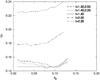 |
Fig. 3 Behavior of simulations of binary formation, compared to observations. Several slopes (the “t” parameter) of initial mass functions are shown. The IMFs with smaller slopes, together with 0.06 ≤ q0 ≤ 0.1, provide the best fits. |
5. Discussion and concluding remarks
An inspection of Fig. 1 does not provide evidence of a period dependency on the Y distribution and, therefore, the form of f(q) does not seems to be period-dependent. An analogous histogram is found in Fisher et al. (2005), with a different shape; indeed, since the criteria used to compile the samples are very different, a similarity is not expected. The question of the form of the mass ratio distribution in spectroscopic binaries as well as on the q0 value can be addressed by an analysis of Fig. 2, where the histogram of the entire sample of 249 stars was compared with the various simulations; similar calculations using the subsamples for shorter and longer periods did not produce significantly different results. We analysed the evolution of D values because several q0 are used in each q distribution. From Fig. 2 it is clear that those q distributions that are bimodal or increase with q, have higher D, regardless of which q0 is used. Therefore, this family of functions is unsuitable for the present simulations. Another group of functions seems to provide better fits. A mass ratio distribution with uniform probability (function 1) gives good results. However, linear, decreasing q functions in the form f(q) = 1 − aq with a ≈ 0.5, produce the best fits to observations, and also give important information on the q0 value, which is around 0.08. These functions are preferred over function 1 because they provide information on the constraint on q0, while function 1 only returns low D values for unphysical (i.e. too low) values of q0. Function 5 with a = 0.5 seems to be the best compromise between low D and a physical q0. Consequently estimates of q0 around 0.2 do not produce the best results. A q0 from 0.08 to 0.1, meaning that one component can be more than ten times more massive than the other, puts limits on the primary masses, giving preference to the formation of systems with non-massive primaries, and where both components, with low masses and slower evolutionary rates, can coexist as main-sequence stars. An examination of the observational sample shows that 29% of the primaries are OB stars; even if this frequency is higher than the frequency of OB stars in the Galaxy, it must be stressed that the sample may carry a bias toward brighter younger stars because it was limited to stars brighter than mV = 7.0. This strongly suggests that the majority of SBs is composed of low-mass stars, and that a q0 limit around 0.1, allowing simultaneous main sequence components, is the best fit to observations.
Considering the initial mass functions for spectroscopic binaries, Fig. 3 shows that steeper slopes, around 2.35, are not the best fits to observations. Indeed, slopes of about 1.4 seem
to be more adequate, even when combined with steeper ones. With respect to q0, differences between the three curves at the bottom of Fig. 3 are small, with slight advantage to the homogeneous distribution with slope 1.4, which has its minimum around q0 = 0.08 to q0 = 0.1, reinforcing the perception gained in the former paragraph. So, a reasonably good fit to observations is obtained from the pairing of stars that are independently formed; the standard IMF is not followed, which suggests an alternative process of binary formation, different from that of single field stars. The process of fragmentation, which is defined as break-up occurring during the dynamical collapse phase of protostellar clouds, leading to equal mass binaries and a dominance of high mass-ratios (Boss 1988), is not confirmed by the present study, because the best fit to observations comes from models with mass ratio distributions favoring low values of q. Processes of spectroscopic binary formation, as expected, are different from those of visual binaries.
Observational data. Column headings: system identification, primary spectral type, primary mass, primary magnitude, system period (days), system orbital excentricity, primary radial velocity (km s-1), mass function, Y value (from Eq. (4)); in last column, a “II” marks SBII systems.
References
- Abt, H. A., & Levy, S. G. 1976, ApJS, 30, 273 [NASA ADS] [CrossRef] [Google Scholar]
- Abt, H. A., & Levy, S. G. 1985, ApJS, 59, 229 [NASA ADS] [CrossRef] [Google Scholar]
- Batten, A. H., Fletcher, J. M., & Mann, P. J. 1978, Pub. Dominion Astrophys. Obs. 15, 121 [Google Scholar]
- Boss, A. P. 1988, Comments Astrophys. 12(4), 169 [Google Scholar]
- Dabrowski, J. P., & Beardsley, W. R. 1977, PASP, 89, 227 [NASA ADS] [Google Scholar]
- Duquennoy, A., & Mayor, M. 1991, A&A, 248, 485 [NASA ADS] [Google Scholar]
- Fekel, F. C., Gillies, K., Africano, J., & Quigley, R. 1988, AJ, 96, 1426 [NASA ADS] [CrossRef] [Google Scholar]
- Figer, D. F. 2005, Nature, 434(7030), 192 [NASA ADS] [CrossRef] [PubMed] [Google Scholar]
- Fisher, J., Schroder, K. P., & Smith, R. C. 2005, MNRAS, 361, 495 [NASA ADS] [CrossRef] [Google Scholar]
- Garmany, C. D., Conti, P. S., & Massey, P. C. 1980, AJ, 242, 1063 [Google Scholar]
- Giannone, P., & Giannuzzi, M. A. 1969, Ap&SS, 84, 292 [Google Scholar]
- Goodwin, S. P., & Kroupa, P. 2005, A&A, 439, 565 [NASA ADS] [CrossRef] [EDP Sciences] [Google Scholar]
- Halbwachs, J. L. 1987, A&A, 183, 234 [NASA ADS] [Google Scholar]
- Heacox, W. D. 1998, AJ, 115, 325 [NASA ADS] [CrossRef] [Google Scholar]
- Hogeveen, S. J. 1990, Ap&SS, 173, 315 [NASA ADS] [CrossRef] [Google Scholar]
- Hogeveen, S. J. 1992a, Ap&SS, 193, 29 [NASA ADS] [CrossRef] [Google Scholar]
- Hogeveen, S. J. 1992b, Ap&SS, 196, 299 [NASA ADS] [CrossRef] [Google Scholar]
- Iben, I. Jr. 1964, ApJ, 140, 1631 [NASA ADS] [CrossRef] [Google Scholar]
- Jaschek, C. 1969, Arch. Sc. Geneve, 24(1), 167 [Google Scholar]
- Jaschek, C., & Ferrer, O. 1972, PASP, 84, 292 [NASA ADS] [CrossRef] [Google Scholar]
- Kennicut, R. C. 1998, in The Stellar Initial Mass Function, ed. G. Gilmore, & D. Howell, ASP Conf. Ser., 142, 1 [Google Scholar]
- Lang, K. R. 1991, Astrophysical Data: Planets and Stars (Springer), 133 [Google Scholar]
- Larson, R. B. 2001, PASP, in The Formation of Binary Stars, , ed. H. Zinnecker, & R. D. Mathieu (Potsdam), Proc. IAU Symp., 200, 3 [Google Scholar]
- Levato, H., Malaroda, S., Morrell, N., & Solivella, G. 1987, ApJS, 64, 487 [NASA ADS] [CrossRef] [Google Scholar]
- Lucy, L. B., & Ricco, E. 1979, AJ, 84, 401 [NASA ADS] [CrossRef] [Google Scholar]
- Pourbaix, D., Tokovinin, A. A., Batten, A. H., et al. 2004, A&A, 424, 727 [NASA ADS] [CrossRef] [EDP Sciences] [Google Scholar]
- Salpeter, E. E. 1955, ApJ, 121, 161 [Google Scholar]
- Staniucha, M. 1979, Acta Astron., 29(4), 587 [NASA ADS] [Google Scholar]
- Tohline, J. E., & Durisen, R. H. 2001, PASP, in The Formation of Binary Stars, ed. H. Zinnecker, & R. D. Mathieu (Potsdam), Proc. IAU Symp., 200, 40 [Google Scholar]
- Tout, C. A. 1991, MNRAS, 250, 701 [NASA ADS] [CrossRef] [Google Scholar]
- Trimble, V. 1974, AJ, 79, 967 [NASA ADS] [CrossRef] [Google Scholar]
- Trimble, V. 1990, MNRAS, 242, 79 [NASA ADS] [Google Scholar]
- Trimble, V., & Ostriker, J. P. 1978, A&A, 63, 437 [NASA ADS] [Google Scholar]
- Warren Jr, W. H., & Hoffleit, D. 1987, BAAS, 19, 733 [NASA ADS] [Google Scholar]
All Tables
List of mass ratio, q distributions used in the construction of histograms for theoretical Y.
Observational data. Column headings: system identification, primary spectral type, primary mass, primary magnitude, system period (days), system orbital excentricity, primary radial velocity (km s-1), mass function, Y value (from Eq. (4)); in last column, a “II” marks SBII systems.
All Figures
|
Fig. 1 Histogram for observed Y, from 249 spectroscopic binaries (solid line). Also shown are normalized tracings of sub-samples, for periods longer (dotted line) or shorter (dot-dashed line) than 40 days. |
| In the text | |
|
Fig. 2 Behavior of simulations of binary formation, compared to observations. Several mass distributions from Table 1 are shown. Distributions favoring lower mass ratios and values of q0, the minimal mass ratio around 0.08 provides the best fits. |
| In the text | |
|
Fig. 3 Behavior of simulations of binary formation, compared to observations. Several slopes (the “t” parameter) of initial mass functions are shown. The IMFs with smaller slopes, together with 0.06 ≤ q0 ≤ 0.1, provide the best fits. |
| In the text | |
Current usage metrics show cumulative count of Article Views (full-text article views including HTML views, PDF and ePub downloads, according to the available data) and Abstracts Views on Vision4Press platform.
Data correspond to usage on the plateform after 2015. The current usage metrics is available 48-96 hours after online publication and is updated daily on week days.
Initial download of the metrics may take a while.