| Issue |
A&A
Volume 524, December 2010
|
|
|---|---|---|
| Article Number | A10 | |
| Number of page(s) | 8 | |
| Section | Catalogs and data | |
| DOI | https://doi.org/10.1051/0004-6361/201015315 | |
| Published online | 19 November 2010 | |
Towards a new full-sky list of radial velocity standard stars⋆
1
GEPI, Observatoire de Paris, CNRS, Université Paris Diderot,
5 place Jules Janssen,
92190
Meudon,
France
e-mail: This email address is being protected from spambots. You need JavaScript enabled to view it.
2
UMR CNRS/UM2 GRAAL, CC 72, Université Montpellier2,
34095
Montpellier Cedex 05,
France
3
Université Bordeaux 1, CNRS, LAB, 33270
Floirac,
France
4
Observatoire astronomique, Université de Strasbourg, CNRS, 11 rue
de l’Université, 67000
Strasbourg,
France
5
Astrophysikalisches Institut Potsdam, Potsdam, Germany
6
Observatoire de Genève, 51 Ch. des Maillettes, 1290
Sauverny,
Switzerland
7
Institut d’Astrophysique Spatiale, Université Paris-Sud,
91405
Orsay Cedex,
France
Received:
1
July
2010
Accepted:
12
August
2010
Abstract
Aims. The calibration of the Radial Velocity Spectrometer (RVS) onboard the ESA Gaia satellite (to be launched in 2012) requires a list of standard stars with a radial velocity (RV) known with an accuracy of at least 300 m s-1. The IAU commission 30 lists of RV standard stars are too bright and not dense enough.
Methods. We describe the selection criteria due to the RVS constraints for building an adequate full-sky list of at least 1000 RV standards from catalogues already published in the literature.
Results. A preliminary list of 1420 candidate standard stars is built and its properties are shown. An important re-observation programme has been set up in order to insure within it the selection of objects with a good stability until the end of the Gaia mission (around 2018).
Conclusions. The present list of candidate standards is available at CDS and usable for many other projects.
Key words: catalogs / stars: kinematics and dynamics / techniques: radial velocities
Complete Table 2 is only available in electronic form at the CDS via anonymous ftp to cdsarc.u-strasbg.fr (130.79.128.5) or via http://cdsweb.u-strasbg.fr/cgi-bin/qcat?J/A+A/524/A10
© ESO, 2010
1. Introduction
Since the first catalogue of stellar radial velocities published by Moore (1932), the number of measured stellar radial velocities (RV) has increased considerably, thanks to the very wide uses of these data, from galactic dynamics to stellar atmospheric motions and the discovery of extra-solar planets. The General Catalogue of stellar Radial Velocity (GCRV, see Wilson 1953) has been used for many different purposes. Today, very extensive RV surveys are in progress, like the Radial Velocity Experiment (RAVE project, see Steinmetz et al. 2006), or the SDSS-SEGUE survey (see Yanny et al. 2009); or in preparation, like the Gaia-RVS (see Katz 2009), and the LAMOST survey (see Newberg & LAMOST project of China and Participants in LAMOST (PLUS) 2009). Each of these surveys has its own scientific goals, but all need a wavelength calibration which guarantees the quality of spectroscopic data, particularly radial velocities (RV) and rotational velocities. These calibrations rely on the radial velocity zero-point (RVZP) of the instruments, which can evolve with time during the life of the project. A way to take care of these RVZP is the continuous observation of “standard” stars and/or “reference” objects such as asteroids. The concept of “standard star” and “set of standards” has been carefully examined by Batten (Batten 1985a,b) and is based on the physical notion of “stability”; this notion of “stability” is of course limited by other physical concepts (for the fundamental definition of radial velocity, see Lindegren & Dravins 2003) and is very dependent on the accuracy expected for the project. It is the reason why each project, whether ground-based or space-based, has to establish an appropriate list of such “standard stars”.
In this paper we discuss the construction of a new full-sky list of candidate RV standard stars developed specifically within and for the Gaia project, but which will hopefully be very useful for many other astronomical projects. Indeed, this list of rather bright stars is established for the RVS (Radial Velocity Spectrometer) survey on board the Gaia satellite (see Katz et al. 2004), which will use it in close interaction with asteroids for its RVZP. The strategy for building this list is somewhat different from that adopted by the Space Interferometry Mission (SIM project, see Frink et al. 2001), which plans to build a reference astrometric grid over the whole sky by means of radio-loud quasars and a “Grid Giant Star Survey” composed of RV-stable red K giant stars (Bizyaev et al. 2006). While the large ground-based RV-surveys like SDSS-SEGUE, RAVE or the ELODIE Archive (see Moultaka et al. 2004) use calibration lamps permanently installed on the instrument to determine the wavelength scale, standard stars also allow to check the good status of the spectrograph such as stability or possible slow drifts.
The process of building this list in addition to the official IAU commission 30 lists (available at: http://obswww.unige.ch/~udry/std/std.html) may be compared to the similar but much older process in astrometry: a short basic list of very bright stars with very accurate positions, like the FK series of astrometric catalogues; supplemented by larger and denser lists of fainter objects, like the AGK catalogues.
We discuss first the former lists of RV standard stars and the available data for building a new larger one. Then we describe in detail the constraints and criteria adopted, the way we have selected the candidate stars, and the properties of the resulting list. Finally we develop the on-going strategy for re-observing our sample in both hemispheres.
2. The IAU commission 30 lists of RV standards
IAU commission 30 has set up a working group devoted to RV standards. Two lists of standards are available at the above address:
-
CORAVEL standard stars, with only a limited accuracy(on the order of300 m s-1; some much worse); 107 objects;
-
“New” ELODIE-CORAVEL high-precision standard stars: 37 objects, with 0.57 ≤ B − V ≤ 0.94, and an accuracy of about 50 m s-1.
These objects have been repeatedly observed for years, and will constitute a firm basis for a new list. However they are not numerous enough for the RVS: only 144 objects, most of them too bright for the RVS (see Fig. 1).
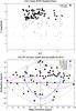 |
Fig. 1 Properties of the IAU commission 30 RV standard stars. Top: distribution in the colour-magnitude plane. Stars brighter than V = 6 (small open circles) are too bright for RVS standards, and will therefore not be kept for our list. Filled circles indicate IAU standards fainter than V = 6, suitable for RVS. Bottom: sky distribution of the IAU standards (symbols as for the top panel). A large fraction of the usable standards is located in a strip around δ = + 30°, with a clear lack of standards in the southern hemisphere. |
It is therefore necessary to search for more “standards”, which have of course a shorter observational history.
We note that several former “stable” stars in these lists recently revealed to be variable with an amplitude about a hundred of m s-1 thanks to the use of very high-precision spectrometers such as CORALIE (see Udry et al. 2000) and HARPS (see Pepe et al. 2000), devoted to the search of extrasolar planets.
3. Constraints due to the Gaia-RVS
The Gaia RVS is an integral-field spectrograph with no calibration device onboard owing to payload size and weight constraints. Therefore calibration sources must be found among the many programme objects and used as references. For the RVS, the best objects are the asteroids; unfortunately only very few are bright enough, and their distribution across the sky is not uniform because they are concentrated in the vicinity of the ecliptic. Although they are the ultimate references (their RV can be accurately calculated from celestial mechanics), they must be supplemented by a list of suitable stars. Descriptions of the RVS may be found in Katz et al. (2004), and in Katz (2009) for an up-to-date description.
In this paper, we present the construction of the list of possible standards for the RVS instrument. Our selection, based on available ground-based data, is performed according to criteria tuned for the Gaia-RVS specific needs, like the RVS geometry, its feeding and read-out system as well as the Gaia scanning law, leading to specific constraints. These requirements will just be listed for a good unterstanding of the procedure; but they will not be established nor developed here. The resulting list can be used totally independently of the RVS for many different purposes, because it covers the whole sky.
3.1. Magnitude range
Very bright stars are not taken into account for RVS instrumental configuration; and faint stars with a low S/N have a low accuracy and cannot be used as references. The RVS spectral interval 847 − 874 nm is contained in the I band. The magnitude over this small interval is denoted GRVS, and can be expressed as a polynomial transformation equation between the usual V magnitude and the Cousins’ I, or IC magnitude. The magnitude limitations are of course given primarily in GRVS. The magnitude range for the RVS standard stars is defined as:
-
bright end: V = 6.0 (on-board limitation);
-
faint end: GRVS = 10.0, corresponding to V ~ 11 for K1III giants.
3.2. Size of the list
Some 1000 standard stars are needed for a best performance of the RVS reduction algorithm (Guerrier 2008). However, this is the number of stars aimed at in the final list: given that some of the presently selected stars will not satisfy all the constraints, in particular those concerning binarity and variability, it was decided to extend the size of the candidate standard stars to some 1500 objects. All these stars are re-observed before and during the mission; some will be dropped from the present list, and the final list to be kept will be known only at the end of the Gaia mission, around 2018. We nevertheless expect to have a good first selection at Gaia launch time (around the end of 2012).
3.3. Initial accuracy in radial velocity
The final accuracy on RVS velocities is expected to be of the order of 1 km s-1 for the brightest stars. Therefore standard stars must be known a priori with a better accuracy, and the initial limit for selection was set to 300 m s-1; reducing it to 100 m s-1 would have been a criterion too hard to fit, as less than the 1500 stars required were known with such an accuracy when the search was begun. The remeasurement programme undertaken should allow us to have at Gaia launch time a precision of the order of 100 m s-1 for the whole list.
3.4. Spectral range and spectral type range used
The RVS spectral range is 847–874 nm; the choice of this small and up to now unusual range for RV is described in Munari (1999); see also Katz et al. (2004); it covers the three lines of the IR CaII triplet, which are visible in most stellar types, roughly B8 to M5V. Moreover, in late-type stars it contains many narrow metallic lines, which are extremely useful for a good fit of the dispersion all along the range; and in early-type stars several Paschen lines are visible. Numerical simulations performed with IRAF over synthetic spectra show that the RV accuracy is reduced for stars earlier than F5. Notice that if K-type red giants are very “good” stars with sharp lines, it was found by Bizyaev et al. (2006) during their preparatory study for the SIM mission that the best stable giants should satisfy 0.59 < (J − Ks) < 0.73 (roughly G7 to K2 giants). We will keep this constraint, converted into our colour indices, in order to eliminate possible variables (see below).
3.5. Photometric variability
Variable stars are a real problem, irrespective of the cause of the variability: motions in the atmosphere, or close companions. In all cases, the variability may be a reason for “unstable” radial velocity. Therefore all objects with an indication of variability in the Hipparcos Catalogue (Perryman et al. 1997) have been discarded, because we need objects stable until the end of the mission (2018).
3.6. Multiplicity
Double stars must be eliminated as much as possible; all stars with some indication of multiplicity have been deleted, even those with a long period, because stability of RV is required until the end of the mission. The RV lists and catalogues used have been carefully searched for indications of multiplicity. However some double stars are certainly still contained in our list. The ongoing re-observations should allow us to eliminate most of them.
3.7. Neighbourhood
Because the RVS is a slitless spectrograph, somewhat comparable with the former objective prism spectrographs, the spectra of the different stars may overlap in the focal plane, depending on the angular distance of the objects and the orientation of the dispersion. The overlap may disturb the main spectrum, inducing an error in the derived RV. Because each star will be observed around 40 times during the mission, with various orientations for the scanning direction, we discarded stars with bright neighbours (ΔI < 4 ) within a circle of radius just above the size of a spectrum on the detector (ρ < 80″). This condition led to the deletion of many otherwise “good” stars, particularly in dense areas such as the vicinity of Galactic Plane. As discussed below (see Sect. 4.4), in a few cases it was necessary to slightly relax this constraint.
3.8. Hipparcos stars
We also felt that all the RVS standard stars should be in the Hipparcos catalogue (see Perryman et al. 1997). This allows the use of only a few common criteria over very homogeneous data acquired over the full sky with a unique instrument: magnitudes, variability, indications of multiplicity or close neighbours. The Hipparcos magnitudes and colours V and V − I are also used to calculate GRVS, even if the V − I colours are not perfect (see Platais et al. 2003).
A (small) drawback is the magnitude distribution of the Hipparcos stars, which drops strongly beyond V = 9; however the RV catalogues used below contain mostly HIP stars, so that the real loss due to this requirement is not very important.
3.9. Hipparcos master list
A first list was extracted from the Hipparcos Catalogue, taking into account all the above criteria, except those on neighbourhood and initial RV accuracy. It contains some 42 109 stars, with no RV indication. Some newly recognized doubles found in the SIMBAD data base were then removed.
Then the problem of neighbourhood was handled with use of USNO-B1 catalogue, which is available on-line at CDS Strasbourg; it contains an I magnitude for most objects. Each star of the above list was examined in the USNO-B1 catalogue, and all its neighbours within 80 arcsec and brighter than I = 15 were retrieved. Because for the faintest stars an I magnitude is not always available, but only B and R, it was roughly estimated by: I = R − 0.34 × (B − R) (empirical relation established with the bright stars). Of course this treatment is not totally rigorous; it was however considered as the best one, owing to the complexity of the problem. If some stars are not really good, the ongoing re-observation programme should help eliminate most of them. It should be noted that the HIP stars eliminated through this “neighbourhood condition” are of course more numerous in dense areas, particularly in the vicinity of the Galactic Plane.
The choice of USNO-B1 (see Monet et al. 2003) catalogue was motivated by the following considerations: full-sky coverage; very large number of stars; very large magnitude range, with the bright stars being taken from the Tycho-2 catalogue; availability of I magnitude for most stars handled (I ≤ 15); good access to the on-line catalogue at CDS Strasbourg through the Vizier interface. A recent partial check on southern selected stars based on the newly-available UCAC3 (see Zacharias et al. 2009) showed that only a very small fraction of retained stars still had disturbing neighbours not listed in USNO-B1; however the UCAC3 has a smaller magnitude range and lacks I magnitudes for most of the stars.
All stars satisfying the above neighbourhood conditions were kept. The resulting list of 38 169 HIP stars is the “master list”: only stars within it can be accepted. Stars selected afterwards from RV criteria will be considered as usable only if they are in this master list. However, as will be shown below (see Sect. 4.4), it will be necessary in a few cases to take stars not found in the master list because of too many disturbing neighbours.
4. Selection among existing published RV catalogues
Several recently published catalogues of reliable RV have been examined. The aim is to cover the sky roughly homogeneously with accurate data coming from only a smallnumber of spectrographs, which have some stars in common. Therefore, although many recent catalogues are available in the literature, only three were retained beside the official IAU standards: those of Nidever et al. (2002), Nordström et al. (2004), and Famaey et al. (2005). All have different presentations, qualities and parameters; and the selection must be adapted to each one. The intersection with our master list allows us to concentrate on only RV criteria; the others are automatically fulfilled.
For reading and citation convenience, these catalogues will be denoted below: NID, NOR, FAM, in addition to IAU.
4.1. The Nidever et al. (2002) catalogue = NID
This catalogue contains 889 stars observed during four years between 1997 and 2001, and 782 exhibit velocity scatter smaller than 0.1 km s-1. Nonetheless, “... they suffer from three sources of systematic errors, namely convective blueshift, gravitational redshift, and spectral mismatch of the reference spectrum... The spectra were obtained with the HIRES spectrometer on the 10 m Keck-1 telescope, and with the Hamilton echelle spectrometer fed either by the 3-m Shane or the 0.6 CAT...” (as taken from the Catalogue’s Read-Me at CDS, Vizier section). Calibration was done by iodine vapour lines superimposed over the stellar lines. Each programme star has an average of 12 observations.
Only the HIP stars of their Table 1 have been taken into account (stable stars with rms ≤ 100 m s-1, 742 rows). Of them, only 329 are in our “master list”, mainly due to the requirement of neighbourhood.
We note that the “three sources of systematic errors” mentioned above may apply as well to the other catalogues.
4.2. The Nordström et al. (2004) catalogue = NOR
This catalogue (“The Geneva-Copenhagen survey of the solar neighbourhood”) contains a complete, magnitude-limited, and kinematically unbiased sample of 16 682 nearby F and G dwarf stars. Complete kinematic information for 14 139 stars is taken from Hipparcos/Tycho data, and complemented by new, accurate radial-velocity observations for most of the stars. The aim was to obtain new determinations of metallicity, rotation, age, kinematics, and Galactic orbits for this sample, and new isochrone ages for all stars for which this is possible. The number of RV observations used and the corresponding time span are available for each star.
From Table 1 of the NOR catalogue we extracted the HIP stars with at least 2 RV observations, mean error and standard deviation on RV smaller than 0.3 km s-1, and considered as single by the authors: 3227 stars before intersection with our “master list”, all with RVs obtained with CORAVEL, north and south. 1696 stars have only two measurements, and 1531 have at least three. 1039 stars with at least three measurements are in the master list.
4.3. The Famaey et al. (2005) catalogue = FAM
This catalogue provides Hipparcos positions, Hipparcos and Tycho-2 proper motions, and CORAVEL radial velocities for 6691 K and M giants in the solar neighbourhood, mostly from the Hipparcos survey (northern hemisphere only). It is intended for deriving the kinematics of giant stars in the solar neighbourhood, and to correlate it with their location in the Hertzsprung-Russell diagram. Binaries for which no centre-of-mass velocity could be estimated have been excluded; but known binaries remain, and will have to be eliminated. The primary sample includes 5952 K giants and 739 M giants. 86% are in the Hipparcos “Survey” (for the definition of the Hipparcos Survey, see Crifo et al. (1985). Useful complementary data on the radial velocities, not available in the published tables (number of measurements, time span between first and last observation) were sent very kindly by B. Famaey. As most of these stars have only a small number of RV measurements, the Bizyaev criterion (Bizyaev et al. 2006) was applied in order to increase the probability of retaining stable giants; with the available colours at our disposal this criterion may be converted into: 0.9 < B − V < 1.2. Only the FAM stars are concerned: the NID stars have many more observations, and only “stable” stars have been selected; the NOR stars include no giants. Before intersection with our “master list”, 1586 FAM stars satisfied this criterion (K giants only). Of them, 1449 stars have only two measurements, and 137 have at least three. 126 stars with at least three measurements are in the master list.
4.4. Resulting list
In a first step, only single stars of the 4 RV-catalogues (IAU, NID, NOR, FAM) with an RV accuracy better than 0.3 km s-1, and at least three existing measurements within the NOR and FAM catalogues were kept and cross-matched with our “master list”; the result is a list of 1342 stars, a sufficiently large number of objects for our purpose; but some regions of the sky were not very well covered, particularly the vicinity of the galactic plane. The selection criteria for neighbourhood were therefore slightly relaxed (vicinity distance down to 60″ instead of 80″ for 3 ≤ ΔI ≤ 4, after numerical simulations); also in some places, stars with only two existing RV measurements from NOR or FAM had to be taken in order to fill the gaps. This supplementary list (not all in the the master list) was selected by hand and contains only 78 objects. Of course these stars must be re-observed in priority, with two new measurements before Gaia launch.
The current list of candidate standard stars contains 1420 stars. Some stars are common to two or even three RV lists and are therefore particularly useful. Notice that some stars might be rejected in the future, after more remeasurements are performed.
5. Statistical properties of the list
5.1. Sky distribution
The full sky distribution for these 1420 stars is shown in Fig. 2, with different symbols for the 1342 best and 78 supplementary stars. The gaps in the vicinity of galactic plane are not perfectly filled.
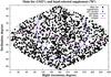 |
Fig. 2 Map of the selected stars: full circles are the 1342 best stars; triangles are the 78 slightly less good ones selected by hand in the gaps, mostly near the galactic plane. |
Figure 3 shows the origin of the selected stars, according to the following hierarchical order for stars found in various lists: IAU; NID; NOR; FAM. Stars found in several lists are plotted according to their highest-priority list.
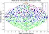 |
Fig. 3 Origin of the selected stars per list. Most of them are from NOR, especially in the south, thanks to the southern CORAVEL. |
5.2. Distribution in magnitude
Figure 4 shows the histogram in V magnitude: its mode is at about 8.1, slightly lower than in Hipparcos (8.6); this difference is due mainly to the important effort in the Hipparcos catalogue for reducing the total number of cool stars and particularly the red giants included in the so-called “ Hipparcos survey” (see Crifo et al. 1985); and here we take only cool HIP stars.
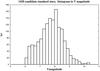 |
Fig. 4 The list of 1420 candidates: histogram in V magnitude. |
5.3. Distribution in colour
Figure 5 shows the HR diagram of the stars, with the same colour code as for the map of Fig. 3. The separation between the various origins is very clear. Most giants are from FAM, and therefore occupy an area limited by the Bizyaev criterion.
5.4. Distribution in Radial Velocities
Figure 6 shows the distribution in radial velocities vs. (V − I)HIP. The highest RVs come from NOR; but are nevertheless not extremely high (only one star above 150 km s-1).
6. Comparison between the different lists
Our list is made out of four previously existing lists. These have several stars in common, but with data obtained with different instruments.
Table 1 shows the numbers of common stars. It also gives the number of stars retained within each original catalogue. These numbers are slightly larger than those given for the intersection with the master list, due to the supplementary list of 78 stars.
It is interesting to compare the data of the common stars. IAU standards are of course taken as references; but they have quite small intersections with other lists. Only 13 stars are common to IAU, NID and NOR; and the FAM stars contain only 3 IAU stars, not found in the other lists. Figure 7 shows these 13 common stars, plus the 3 FAM stars.
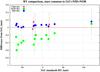 |
Fig. 7 The 13 stars common to IAU, NID and NOR; plus the 3 IAU/FAM stars, all compared to IAU RV. |
The offset between NID+FAM and IAU is quite small (0.063 km s-1); but the NOR data for the same objects show a larger offset, and with larger error bars due to the less accurate CORAVEL measurements.
Because the samples involved in Fig. 7 are very small, we investigated the differences between the NOR, FAM and NID data more in detail, taking now the NID stars as references. For NOR vs. NID we took the 163 common objects of Table 1. For FAM vs. NID: as the number of common stars is again very small (only 3, see Table 1), we tried to increase this number by comparing the lists before their intersection with our master list. A set of 25 common stars could be defined that way, including the 3 ones of Table 1. In Fig. 8 the differences in RV (FAM – NID) and (NOR – NID) are plotted versus B − V. Although the FAM stars cover only a small interval in B − V, they clearly agree well with NID, while the NOR data show a trend in B − V.
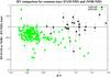 |
Fig. 8 Comparison of NOR and FAM with NID, vs. B − V. The 163 stars common to NOR and NID are those of Table 1, and the 25 stars common to FAM and NID are taken before intersection with the master list. |
Numbers of stars common to various lists.
These results are derived from the published data. However, the NOR and FAM data are for a good part obtained with the same instrument (northern CORAVEL, located at OHP, France), and are handled in the same Coravel database. It appears that the NOR data, which were obtained and published before the FAM ones, experienced an earlier reduction in the database; and a small change in the scale was introduced between the two sets. The recent updates of the NOR catalogue by Holmberg et al. (Holmberg et al. 2007, 2009) did not update the radial velocities. Clearly, the new scale used for the FAM data allows a much better agreement with the NID data. For the final RVS list, we will use the NOR data re-reduced with the new scale.
The offsets seen in Figs. 7 and 8 reveal the differences of RVZP proper to each instrument and reduction procedure related to resolution, wavelength ranges, calibration lamps, line lists, numerical tools for fitting the lines, template/masks (models) used for the correlation function (K0, G5, G2) etc. The aim of the observing programme that we have started to follow-up the list of candidates is not only to check the RV stability of the stars, but also to define a common RV scale based on asteroids (see next section). As a consequence our final catalogue of RV standards will be homogeneous, with an absolute RVZP.
7. Re-observation programme
From the list of 1420 candidates, at least 1000 RV-STD stars will be selected. These primary stars have to be stable in radial velocity at the 300 m s-1 level, with no drift until the end of the mission (2018). To be qualified as a RVS standard star, each candidate has to be observed at least twice until the late mission phase in order to verify its long term stability.
Our observational strategy has been defined to respond to the following constraints:
-
Checking the 300 m s-1 stability implies a RV accuracy of individual measurements better than 100 m s-1, which is easily obtained with modern echelle spectrographs and FGK stars, without requiring a high signal-to-noise ratio.
-
To cover the whole sky, we need to use northern and southern instruments, which implies checking the consistency between the different instruments and to set the zero-point scale. Asteroids and IAU standards are systematically observed for that purpose.
-
The NID list is supposed to be already cleaned of non-stable stars at the level of 100 m s-1. Only one supplementary observation is needed before launch to verify the stability of NID candidates.
-
FAM and NOR catalogues rely on CORAVEL measurements, which have a typical uncertainty of 300 m s-1. Moreover most candidates have only three or even two RV measurements available. At least two supplementary observations are mandatory to check their stability before launch.
-
For all non-rejected candidates at the time of launch, one more observation during the mission has to be done to reject stars with long-term variations.
To conduct this long-term and extensive programme, three echelle spectrographs are used: SOPHIE mounted on the T193 at OHP, NARVAL mounted on the Telescope Bernard Lyot at Pic du Midi Observatory; and CORALIE mounted on the Swiss Euler Telescope at La Silla.
We have also collected useful measurements in the ELODIE archive (Moultaka et al. 2004), and will search the HARPS archive at ESO.
All these instruments provide RV measurements with an accuracy better than 50 m s-1.
The re-observation programme is going on and should be finished for its main part around mid-2012; then the data have to be compared, and homogeneized between all telescopes, thanks to the use of IAU standards, the stars common to several telescopes, and asteroids. Therefore the observing programme includes the observation of one to four or five asteroids per night. The zero-point adopted for the RV scale will be the spectroscopic RV of asteroids; it is correlated with kinematic radial velocities given by the ephemerides, wich have a typical error of 1 m s-1. However this correlation depends on computed convective shifts in the solar spectrum and physical properties of the asteroids, such as angular diameter, spin, phase... This point will be developed later at the end of the observations.
8. Availability of the list
As already stated in several paragraphs above, the present list is only preliminary; the version to be used during the mission, with probably less objects but new RVs, will be ready for Gaia launch; the final version will be known only at the end of the Gaia mission, around 2018. The present preliminary list of 1420 objects is available at CDS, in the Catalogues section. It contains only already published data, extracted from the various original catalogues described above. A subset is given in Table 2. Only the data needed for a good identification are kept, plus the radial velocity data from the various original sources, and the way it was introduced here: the main list of 1342 stars, or the supplementary list of 78 stars.
Extract of the preliminary list of new RV standards, available at CDS in electronic form.
9. Conclusion
A new preliminary full-sky list of candidate Radial Velocity standard stars has been established, containing 1420 HIP stars with a present accuracy of 300 m s-1 or better at selection, to be improved to 100 or possibly 50 m s-1 after re-observation. The magnitude range of these cool stars is 6 to 11 in V. The stars are well isolated (no disturbing neighbours within 80″, or 60″ in a few cases in dense areas). An important reobservation programme is going on, because the stability in RV has to be guaranteed until the end of the Gaia mission (about 2018). Compared to the existing IAU RV-standards, it is a denser and fainter extension, with a good full-sky coverage. It is designed primarily for the calibration of the Gaia-RVS, but may be used for many other purposes and projects.
Acknowledgments
Apart from the authors, this work was encouraged and supported by all the RVS team, within the Gaia DPAC Consortium (Data Processing and Analysis Consortium, led by F. Mignard); and by the french “Action Spécifique Gaia” led by C. Turon. We warmly thank the staff of CDS-Strasbourg, where most of the data are found, for the SIMBAD, Aladin and Vizier tools, for their so friendly help on all types of subjects, and particularly F. Ochsenbein. It is also a pleasure to thank Dr B. Famaey, for providing us so kindly with additional unpublished data that are very useful for the selection process. Also, this work would be almost useless without the ground-based re-observing programme: the many northern telescope nights at Pic du Midi on Narval, and at Observatoire de Haute Provence (OHP) on SOPHIE are taken in charge by the french National Programmes PNPS and PNCG, with often queue observations made by the local staff. The southern observing nights have been carried out with the CORALIE spectrograph mounted on the swiss Euler Telescope at ESO, La Silla (Chile). Our thanks also go the referee, whose sharp eye detected many inconveniences, and insufficient explanations and justifications.
References
- Batten, A. H. 1985a, in Stellar Radial Velocities, ed. A. G. D. Philip, & D. W. Latham, IAU Colloq., 88, 325 [Google Scholar]
- Batten, A. H. 1985b, in Calibration of Fundamental Stellar Quantities, ed. D. S. Hayes, L. E. Pasinetti, & A. G. D. Philip, IAU Symp., 111, 3 [Google Scholar]
- Bizyaev, D., Smith, V. V., Arenas, J., et al. 2006, AJ, 131, 1784 [NASA ADS] [CrossRef] [Google Scholar]
- Crifo, F., Turon, C., & Grenon, M. 1985, in Hipparcos. Scientific Aspects of the Input Catalogue Preparation, ed. T. D. Guyenne, & J. J. Hunt, ESA SP, 234, 67 [Google Scholar]
- Famaey, B., Jorissen, A., Luri, X., et al. 2005, A&A, 430, 165 [NASA ADS] [CrossRef] [EDP Sciences] [Google Scholar]
- Frink, S., Quirrenbach, A., Fischer, D., Röser, S., & Schilbach, E. 2001, PASP, 113, 173 [NASA ADS] [CrossRef] [Google Scholar]
- Guerrier, A. 2008, Ph.D. Thesis: Calibration des données spectroscopiques de la mission Gaia, Observatoire de Paris, École doctorale d’Astronomie et d’Astrophysique d’Île-de-France, 155 [Google Scholar]
- Holmberg, J., Nordström, B., & Andersen, J. 2007, A&A, 475, 519 [NASA ADS] [CrossRef] [EDP Sciences] [MathSciNet] [Google Scholar]
- Holmberg, J., Nordström, B., & Andersen, J. 2009, A&A, 501, 941 [NASA ADS] [CrossRef] [EDP Sciences] [Google Scholar]
- Katz, D. 2009, in SF2A-2009: Proc. Annual meeting of the French Society of Astronomy and Astrophysics, held 29 June − 4 July 2009 in Besançon, France, ed. M. Heydari-Malayeri, C. Reylé, & R. Samadi, 57 [Google Scholar]
- Katz, D., Munari, U., Cropper, M., et al. 2004, MNRAS, 354, 1223 [NASA ADS] [CrossRef] [Google Scholar]
- Lindegren, L., & Dravins, D. 2003, A&A, 401, 1185 [NASA ADS] [CrossRef] [EDP Sciences] [Google Scholar]
- Monet, D. G., Levine, S. E., Canzian, B., et al. 2003, AJ, 125, 984 [NASA ADS] [CrossRef] [Google Scholar]
- Moore, J. H. 1932, Publications of Lick Observatory, 18, 1 [Google Scholar]
- Moultaka, J., Ilovaisky, S. A., Prugniel, P., & Soubiran, C. 2004, PASP, 116, 693 [NASA ADS] [CrossRef] [Google Scholar]
- Munari, U. 1999, Baltic Astron., 8, 73 [Google Scholar]
- Newberg, H. J., & LAMOST project of China and Participants in LAMOST (PLUS), U. S. 2009, BAAS, 41, 229 [NASA ADS] [Google Scholar]
- Nidever, D. L., Marcy, G. W., Butler, R. P., Fischer, D. A., & Vogt, S. S. 2002, ApJS, 141, 503 [NASA ADS] [CrossRef] [Google Scholar]
- Nordström, B., Mayor, M., Andersen, J., et al. 2004, A&A, 418, 989 [NASA ADS] [CrossRef] [EDP Sciences] [Google Scholar]
- Pepe, F., Mayor, M., Delabre, B., et al. 2000, in SPIE Conf. Ser. 4008, ed. M. Iye, & A. F. Moorwood, 582 [Google Scholar]
- Perryman, M. A. C., Lindegren, L., Kovalevsky, J., et al. 1997, A&A, 323, L49 [NASA ADS] [Google Scholar]
- Platais, I., Pourbaix, D., Jorissen, A., et al. 2003, A&A, 397, 997 [NASA ADS] [CrossRef] [EDP Sciences] [Google Scholar]
- Steinmetz, M., Zwitter, T., Siebert, A., et al. 2006, AJ, 132, 1645 [NASA ADS] [CrossRef] [Google Scholar]
- Udry, S., Mayor, M., Queloz, D., Naef, D., & Santos, N. 2000, in From Extrasolar Planets to Cosmology: The VLT Opening Symposium, ed. J. Bergeron, & A. Renzini, 571 [Google Scholar]
- Wilson, R. E. 1953, General Catalogue of stellar Radial Velocities, VizieR Online Data Catalog, 3021 [Google Scholar]
- Yanny, B., Rockosi, C., Newberg, H. J., et al. 2009, AJ, 137, 4377 [NASA ADS] [CrossRef] [Google Scholar]
- Zacharias, N., Finch, C., Girard, T., et al. 2009, UCAC3 Catalogue, VizieR Online Data Catalog, 1315 [Google Scholar]
All Tables
Extract of the preliminary list of new RV standards, available at CDS in electronic form.
All Figures
|
Fig. 1 Properties of the IAU commission 30 RV standard stars. Top: distribution in the colour-magnitude plane. Stars brighter than V = 6 (small open circles) are too bright for RVS standards, and will therefore not be kept for our list. Filled circles indicate IAU standards fainter than V = 6, suitable for RVS. Bottom: sky distribution of the IAU standards (symbols as for the top panel). A large fraction of the usable standards is located in a strip around δ = + 30°, with a clear lack of standards in the southern hemisphere. |
| In the text | |
|
Fig. 2 Map of the selected stars: full circles are the 1342 best stars; triangles are the 78 slightly less good ones selected by hand in the gaps, mostly near the galactic plane. |
| In the text | |
|
Fig. 3 Origin of the selected stars per list. Most of them are from NOR, especially in the south, thanks to the southern CORAVEL. |
| In the text | |
|
Fig. 4 The list of 1420 candidates: histogram in V magnitude. |
| In the text | |
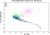 |
Fig. 5 HR diagram of the stars. Colour code and hierarchy for origin as in Fig. 3. |
| In the text | |
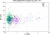 |
Fig. 6 Distribution in radial velocities. Colour code and hierarchy as in Fig. 3. |
| In the text | |
|
Fig. 7 The 13 stars common to IAU, NID and NOR; plus the 3 IAU/FAM stars, all compared to IAU RV. |
| In the text | |
|
Fig. 8 Comparison of NOR and FAM with NID, vs. B − V. The 163 stars common to NOR and NID are those of Table 1, and the 25 stars common to FAM and NID are taken before intersection with the master list. |
| In the text | |
Current usage metrics show cumulative count of Article Views (full-text article views including HTML views, PDF and ePub downloads, according to the available data) and Abstracts Views on Vision4Press platform.
Data correspond to usage on the plateform after 2015. The current usage metrics is available 48-96 hours after online publication and is updated daily on week days.
Initial download of the metrics may take a while.