| Issue |
A&A
Volume 524, December 2010
|
|
|---|---|---|
| Article Number | A23 | |
| Number of page(s) | 8 | |
| Section | The Sun | |
| DOI | https://doi.org/10.1051/0004-6361/201014845 | |
| Published online | 22 November 2010 | |
Selective spatial damping of propagating kink waves due to resonant absorption
1 Departament de Física, Universitat de les Illes Balears,
Spain
e-mail: This email address is being protected from spambots. You need JavaScript enabled to view it.
2 Centre Plasma Astrophysics and Leuven Mathematical Modeling
and Computational Science Centre, Katholieke Universiteit Leuven, Leuven, 3001, Belgium
e-mail: This email address is being protected from spambots. You need JavaScript enabled to view it.
; This email address is being protected from spambots. You need JavaScript enabled to view it.
Received:
22
April
2010
Accepted:
11
August
2010
Abstract
Context. There is observational evidence of propagating kink waves driven by photospheric motions. These disturbances, interpreted as kink magnetohydrodynamic (MHD) waves are attenuated as they propagate upwards in the solar corona.
Aims. We show that resonant absorption provides a simple explanation to the spatial damping of these waves.
Methods. Kink MHD waves are studied using a cylindrical model of solar magnetic flux tubes, which includes a non-uniform layer at the tube boundary. Assuming that the frequency is real and the longitudinal wavenumber complex, the damping length and damping per wavelength produced by resonant absorption are analytically calculated in the thin tube (TT) approximation, valid for coronal waves. This assumption is relaxed in the case of chromospheric tube waves and filament thread waves.
Results. The damping length of propagating kink waves due to resonant absorption is a monotonically decreasing function of frequency. For kink waves with low frequencies, the damping length is exactly inversely proportional to frequency, and we denote this as the TGV relation. When moving to high frequencies, the TGV relation continues to be an exceptionally good approximation of the actual dependency of the damping length on frequency. This dependency means that resonant absorption is selective as it favours low-frequency waves and can efficiently remove high-frequency waves from a broad band spectrum of kink waves. The efficiency of the damping due to resonant absorption depends on the properties of the equilibrium model, in particular on the width of the non-uniform layer and the steepness of the variation in the local Alfvén speed.
Conclusions. Resonant absorption is an effective mechanism for the spatial damping of propagating kink waves. It is selective because the damping length is inversely proportional to frequency so that the damping becomes more severe with increasing frequency. This means that radial inhomogeneity can cause solar waveguides to be a natural low-pass filter for broadband disturbances. Kink wave trains travelling along, e.g., coronal loops, will therefore have a greater proportion of the high-frequency components dissipated lower down in the atmosphere. This could have important consequences for the spatial distribution of wave heating in the solar atmosphere.
Key words: magnetohydrodynamics / waves / magnetic fields / Sun: atmosphere / Sun: oscillations
© ESO, 2010
1. Introduction
The first observations of post-flare transversal coronal loop oscillations by the transition region and coronal explorer (TRACE) (e.g., Aschwanden et al. 1999; Nakariakov et al. 1999; Aschwanden et al. 2002), have inspired much development in magnetohydrodynamic (MHD) wave theory. This observational breakthrough was important since estimated wave parameters, such as frequency and amplitude have allowed us to implement magnetoseismological techniques to probe the plasma fine structure of the Sun’s atmosphere, an idea initially proposed by, e.g., Uchida (1970) and Roberts et al. (1984). It is now commonly accepted that these transversal waves are the kink mode from MHD wave theory (see e.g., Edwin & Roberts 1983), a highly magnetically dominated Alfvénic wave (see Goossens et al. 2009, for a discussion on the nature of kink waves). The observed post-flare kink waves in coronal loops have two main defining characteristics; firstly, they are standing modes, and secondly, they are strongly damped oscillations (in about 1 − 4 periods, see e.g., Aschwanden et al. 2003). Initially there were several physical mechanisms proposed to explain the observed damping, e.g., footpoint leakage (Berghmans & de Bruyne 1995; De Pontieu et al. 2001), lateral wave leakage (Smith et al. 1997; Brady & Arber 2005; Verwichte et al. 2006; Selwa et al. 2005, 2007; McLaughlin & Ofman 2008), phase mixing (Heyvaerts & Priest 1983; Roberts 2002; Ofman & Aschwanden 2002), resonant absorption (Ruderman & Roberts 2002; Goossens et al. 2002), and more recently loop cooling (Morton & Erdélyi 2009). Thus far, resonant absorption, caused by plasma inhomogeneity in the direction transverse to the magnetic field (see Ionson 1978; Hollweg & Yang 1988; Steinolfson & Davila 1993; Ofman & Davila 1995), has proved the most likely candidate for explaining the observed short damping times in coronal loops (see Goossens 2008, for review).
Consistent seismological studies based on resonant absorption using the observed values of periods and damping times of standing kink waves were carried out by Arregui et al. (2007) and Goossens et al. (2008). These two studies show that, at least for a collection of 11 loops, resonant absorption provides an explanation of the observed damping times. The observational signatures of the alternative cooling loop damping mechanism proposed by Morton & Erdélyi (2009) differ from resonant absorption by the fact that the frequency changes as a function of time. The resonant damping theory developed so far is restricted to static and stationary equilibria, and therefore frequency is expected to be constant in time. Extensive MHD modelling has also shown that resonant absorption is the most likely explanation for the damping of transverse oscillations in fine structures of prominences (see Arregui et al. 2008; Soler et al. 2009a,b; Arregui & Ballester 2010).
If indeed, coronal loop kink oscillations are being attenuated by the process of resonant absorption, one can exploit this to estimate the transverse plasma inhomogeneity length scales using observed frequencies and damping times (Goossens et al. 2006). The original equilibrium models by, e.g., Ruderman & Roberts (2002), for studying resonant absorption consisted of monolithic loop structures. However, there has been some observational evidence by, e.g., Aschwanden (2005) that coronal loops are composed of many different strands, possibly at different temperatures and densities. To model this loop multi-thread structure, Terradas et al. (2008) has numerically solved the initial value problem and found that the process of resonant absorption was still an efficient damping mechanism in more complex and realistically structured loop models (see also the work of Ofman 2005). Further study into the properties of standing kink waves has also been undertaken relating plasma inhomogeneity in the direction of the magnetic field caused by, e.g., density (Díaz et al. 2004; Andries et al. 2005b; Arregui et al. 2005; Dymova & Ruderman 2006; Erdélyi & Verth 2007; Verth et al. 2007) or magnetic (Verth & Erdélyi 2008; Ruderman et al. 2008) stratification. It was shown that eigenfrequencies and eigenfunctions of coronal loops with longitudinal stratification were altered in such a way that one could determine, e.g., the coronal density scale height by estimating the ratio of the fundamental mode to that of higher overtones, a technique first proposed by Andries et al. (2005a) and later developed by Verth et al. (2008) to correct for magnetic stratification.
All these theoretical developments to describe kink waves in coronal loops with realistic plasma stratification in the transverse and longitudinal direction were restricted to studying standing waves, since this was what was detected in TRACE data. However, recently it has come to light that there are also ubiquitous small-amplitude, propagating transversal MHD waves in the solar atmosphere. These were first observed by the novel Coronal Multi-channel Polarimeter (CoMP) instrument (Tomczyk et al. 2007). Moreover, Tomczyk & McIntosh (2009) have been able to separate outward and inward propagating wave power. It was found that the outward power was greater than the inward power by about a factor of two, and this can only be explained if the waves are damped in situ (see also Pascoe et al. 2010). The reason we could not detect these propagating waves previously with TRACE is that the amplitudes are of the order of 50 km, while the TRACE resolution is only about 800 km. Tomczyk et al. (2007) originally interpreted these wave as Alfvén waves, but Van Doorsselaere et al. (2008) subsequently argued that the observed waves were actually more consistent with the propagating kink mode. Although both modes are dominated by the restoring force of magnetic tension, in the geometry of a solar flux tube, e.g., a magnetic cylinder, a pure Alfvén wave is strictly torsional with no transverse component and therefore completely incompressible. On the other hand, a kink wave propagating in a flux tube has a transverse perturbation component and is weakly compressible, at least in the linear regime (see e.g., Goossens et al. 2009).
In the present paper, we restrict the study to investigating the effect of transverse plasma inhomogeneity on the propagating kink mode. Although the two problems of standing and propagating kink waves are closely related, since a standing wave is a superposition of two propagating waves, there are some differences that need to be considered. The standing transverse oscillation is the result of an initial value problem, i.e., an initial disturbance in the solar corona such as a CME or a flare, induces the oscillations of the loops at their natural frequencies or eigenmodes. Alternately, the transverse travelling waves have a forced nature since the photosphere acts as a driver. The frequencies of the kink waves observed by CoMP show a peak around 5 min, indicating a p-mode-driven photospheric origin. The spatial scale of the driver at the base of the tube is also important in exciting kink oscillations. From the properties of MHD waves in a flux tube, we know that a purely incompressible excitation excites purely incompressible Alfvén waves if the driver is strictly localised inside or outside the tube (assuming a homogeneous loop model). On the other hand, an excitation located both inside and outside the tube invariably excites transverse oscillations since an almost incompressible surface wave between the two media will be established, i.e., the kink mode.
2. Waveguide model
To understand the effect of radial inhomogeneity on propagating kink waves we consider the relatively simple equilibrium model of a cylindrical axi-symmetric flux tube of radius R with a constant axial magnetic field Bz and with a density contrast of ρi/ρe. The subindexes “i” and “e” refer to the internal and external part of the tube, respectively. It is also assumed that the tube has a smooth variation in density across the waveguide boundary (located at r = R) on a characteristic spatial scale l. For simplicity, a sinusoidal density profile connecting the internal and external part of the tube is implemented (see e.g., Ruderman & Roberts 2002; Goossens et al. 2002; Terradas et al. 2006). The role of the inhomogeneity at the loop boundary is crucial since this is where the process of resonant absorption invariably takes place. This basically means that the transverse displacement of the whole tube is converted into azimuthal motions localised at the tube boundary. The transverse motion is attenuated by this energy conversion, while at the same time small scales are created in the nonuniform layer from phase mixing. Phase mixing causes a cascade of energy to smaller length scales, where the dissipation becomes more efficient. The reader is referred to Goossens (2008), Ruderman & Erdélyi (2009), Terradas (2009), and references therein for further details about this robust damping mechanism. Recent studies by Soler et al. (2009a) in the context of modelling kink oscillations observed in solar prominences (complex coronal magnetic structures with relatively cool and dense plasma) show that the process of resonant absorption still survives even when the plasma is partially ionised.
3. Spatial damping in the TT approximation
Before we embark on analysing MHD waves in the thin tube (TT) approximation, let us explain what this approximation actually is. In what follows we consider both standing and propagating waves. A standing wave is the superposition of two propagating waves travelling with the same frequency and wavenumber but in opposite directions. For the standing wave problem the axial wavelength (or the axial wavenumber kz) is specified and the corresponding frequency is determined. A TT in this case means that the axial wavelength is much longer than the radius of the tube so that kzR ≪ 1, so the TT approximation for standing waves is the long wavelength approximation. The frequency ω is specified for propagating waves and the corresponding wavelength determined. In this situation, a TT means that during one period, defined by the frequency ω, a signal travelling at the Alfvén speed can cross the waveguide in the radial direction many times or ω/(vA/R) ≪ 1. As a result the TT approximation is the low-frequency approximation for propagating waves. The benefit of the TT approximation is that it enables us to obtain simple mathematical expressions that are very accurate, allowing us to gain a physical insight into the problem.
3.1. Homogeneous magnetic cylinder
For a homogeneous magnetic cylinder (i.e., no inhomogeneous layer,
l = 0), the dispersion relation for the kink mode
(m = 1) and the fluting modes (m > 1) in the TT
approximation is (see Goossens et al. 2009)
 (1)where
  (2)The dispersion relation
Eq. (1) specifies a functional dependence
on frequency ω and
wavenumber kz. This can be studied for the
cases of either standing or propagating waves. For the propagating wave study, the
wavenumber kz is specified and the
dispersion relation is solved for frequency ω, leading to the well known
result
(2)The dispersion relation
Eq. (1) specifies a functional dependence
on frequency ω and
wavenumber kz. This can be studied for the
cases of either standing or propagating waves. For the propagating wave study, the
wavenumber kz is specified and the
dispersion relation is solved for frequency ω, leading to the well known
result  (3)where
ω∗ is real. For equal magnetic field strength inside and
outside the cylinder this expression can be further simplified to
(3)where
ω∗ is real. For equal magnetic field strength inside and
outside the cylinder this expression can be further simplified to  (4)For propagating waves
we consider waves generated at a given location with a real
frequency ω∗ and solve the dispersion relation
for kz, resulting in
(4)For propagating waves
we consider waves generated at a given location with a real
frequency ω∗ and solve the dispersion relation
for kz, resulting in  (5)where
k∗ is also real. The solution given by Eq. (5) corresponds to the well known undamped kink
wave (and the fluting modes). To derive Eq. (1) it is implicitly assumed that
ωR/vA ≪ 1, but since not all frequencies
will satisfy these conditions later, we present results for any frequency of driver
without this restriction.
(5)where
k∗ is also real. The solution given by Eq. (5) corresponds to the well known undamped kink
wave (and the fluting modes). To derive Eq. (1) it is implicitly assumed that
ωR/vA ≪ 1, but since not all frequencies
will satisfy these conditions later, we present results for any frequency of driver
without this restriction.
3.2. Inhomogeneous magnetic cylinder
The thin boundary (TB) approximation means that the non-uniformity is confined to
[R − l/2,R + l/2] ,
with l/R ≪ 1, so that the non-uniform layer coincides
with the dissipative layer. This approximation results in the mathematical simplification
that MHD waves can be described by solutions for uniform plasmas that are connected over
the dissipative layer by jump conditions (see e.g., Sakurai et al. 1991; Goossens et al.
1995; Tirry & Goossens 1996). The
use of the TB approximation has been applied in e.g., Goossens et al. (2006, 2009) and Goossens (2008). Including the effect of an
inhomogeneous layer is reasonably simple in the case of the thin boundary approximation
and results in the following dispersion relation,  (6)Here
rA denotes the position of the Alfvén resonance. In the TB
approximation it is natural to adopt rA = R
since l/R ≪ 1 and
rA ∈] R − l/2,R + l/2[.
Using the jump condition is not restricted to the thin non-uniform layer as can be seen
from, e.g., Tirry & Goossens (1996); Tirry et al. (1997, 1998); however, this condition requires numerical integration of the ideal MHD
equations in a non-uniform plasma up to the dissipative layer. In the present paper we do
not intend to use numerical integration of the ideal MHD equations relating to thick
boundaries. However, we do use the results obtained with the TB approximation for thick
boundaries for a comparison with the results of a full numerical calculation in
Sect. 5.
(6)Here
rA denotes the position of the Alfvén resonance. In the TB
approximation it is natural to adopt rA = R
since l/R ≪ 1 and
rA ∈] R − l/2,R + l/2[.
Using the jump condition is not restricted to the thin non-uniform layer as can be seen
from, e.g., Tirry & Goossens (1996); Tirry et al. (1997, 1998); however, this condition requires numerical integration of the ideal MHD
equations in a non-uniform plasma up to the dissipative layer. In the present paper we do
not intend to use numerical integration of the ideal MHD equations relating to thick
boundaries. However, we do use the results obtained with the TB approximation for thick
boundaries for a comparison with the results of a full numerical calculation in
Sect. 5.
The effect of resonance is contained on the right hand side of Eq. (6). Again we can view the dispersion relation
Eq. (6) as a relation for either standing
or propagating waves. In the case of standing waves, the wavenumber is real
(kz = k∗) and
the frequency is complex. This case has been considered previously by e.g., Goossens et al. (1992, 2009). Let us now focus on propagating waves with a given real frequency
(ω = ω∗) and complex wavenumber. The
imaginary part of the wavenumber indicates that the wave, as it propagates, is damped by
resonant absorption. Now we assume that  (7)The purely imaginary
term in Eq. (7) reflects the damping
imposed on the wave, and since the damping is in the spatial domain, the wavenumber is now
complex. If we approximate
(7)The purely imaginary
term in Eq. (7) reflects the damping
imposed on the wave, and since the damping is in the spatial domain, the wavenumber is now
complex. If we approximate  by
by
 (we assume weak damping, i.e.,
kI ≪ kR), we have that
kR ≈ k∗ (given by Eq. (5)), and after some algebra we find
(we assume weak damping, i.e.,
kI ≪ kR), we have that
kR ≈ k∗ (given by Eq. (5)), and after some algebra we find
 (8)Because
 (9)we finally obtain
the following expression
(9)we finally obtain
the following expression  (10)Because
kz is complex, we define the damping length
as LD = 1/kI, while the
wavelength is simply
λ = 2π/k∗. A useful
quantity is the the damping per wavelength, which is
(10)Because
kz is complex, we define the damping length
as LD = 1/kI, while the
wavelength is simply
λ = 2π/k∗. A useful
quantity is the the damping per wavelength, which is  (11)For a sinusoidal
density profile it can be shown that
(11)For a sinusoidal
density profile it can be shown that  (12)and Eq. (11) reduces to
  (13)Equation (13) clearly shows the dependence of the
damping per wavelength on the thickness of the layer. The wider the layer, the stronger
the spatial attenuation of the wave. This is not surprising, since we can relate this
result to the expression for the temporal damping, i.e., wavenumber assumed real
(kz = k∗) and
frequency complex. The well known formula in the case of the temporal damping for a
standing wave is
(13)Equation (13) clearly shows the dependence of the
damping per wavelength on the thickness of the layer. The wider the layer, the stronger
the spatial attenuation of the wave. This is not surprising, since we can relate this
result to the expression for the temporal damping, i.e., wavenumber assumed real
(kz = k∗) and
frequency complex. The well known formula in the case of the temporal damping for a
standing wave is  (14)If we compare this
expression with Eq. (13), we note that the
damping per wavelength for propagating waves and the damping per period for standing waves
are exactly the same so spatial and temporal damping are completely equivalent in the TT
approximation. From Eqs. (13) and (14) we obtain the simple result
(14)If we compare this
expression with Eq. (13), we note that the
damping per wavelength for propagating waves and the damping per period for standing waves
are exactly the same so spatial and temporal damping are completely equivalent in the TT
approximation. From Eqs. (13) and (14) we obtain the simple result  (15)Propagating kink
waves have been recently studied by Vasheghani Farahani
et al. (2009) in the long-wavelength limit in X-ray jets in the solar atmosphere.
These authors computed the ratio of the damping time to the period for standing waves and
use this quantity to discuss the spatial damping of propagating waves. The TT
approximation result presented in Eq. (15)
therefore validates the use of the damping expression derived for kink standing waves by
Vasheghani Farahani et al. (2009) to interpret
the attenuation of propagating kink waves. The TT damping relations given by Eqs. (13) and (14) have other significant consequences. For standing waves, we
rewrite Eq. (14) as
(15)Propagating kink
waves have been recently studied by Vasheghani Farahani
et al. (2009) in the long-wavelength limit in X-ray jets in the solar atmosphere.
These authors computed the ratio of the damping time to the period for standing waves and
use this quantity to discuss the spatial damping of propagating waves. The TT
approximation result presented in Eq. (15)
therefore validates the use of the damping expression derived for kink standing waves by
Vasheghani Farahani et al. (2009) to interpret
the attenuation of propagating kink waves. The TT damping relations given by Eqs. (13) and (14) have other significant consequences. For standing waves, we
rewrite Eq. (14) as  (16)where
  (17)which only depends on the
parameters of the equilibrium model, not on the particular type of MHD wave mode defined
by the value of m. For the kink mode m = 1. The period
is defined by
(17)which only depends on the
parameters of the equilibrium model, not on the particular type of MHD wave mode defined
by the value of m. For the kink mode m = 1. The period
is defined by  (18)and for standing waves
ω is related to the wavenumber
kz by the dispersion relation given by
Eq. (4); i.e.,
(18)and for standing waves
ω is related to the wavenumber
kz by the dispersion relation given by
Eq. (4); i.e.,
 (19)where
vAi is the internal Alfvén speed,
n = 1,2,3,... is the longitudinal mode number, and
L is the total length of the waveguide, e.g., a coronal loop (we have
used that
kz = nπ/L).
Equation (16) can then be written as
(19)where
vAi is the internal Alfvén speed,
n = 1,2,3,... is the longitudinal mode number, and
L is the total length of the waveguide, e.g., a coronal loop (we have
used that
kz = nπ/L).
Equation (16) can then be written as
 (20)where
τAi = L/vAi
is the Alfvén transit time in the longitudinal direction. Equation (20) has interesting consequences. Firstly, it
indicates that fluting modes (m > 1) have shorter damping times
than the kink mode (m = 1). Secondly, it shows that the damping time for
a standing wave is inversely proportional to the longitudinal mode
number n; i.e., the damping time is inversely proportional to the
wavelength of the standing wave, so that higher overtones (with shorter periods) are
damped faster than low-order overtones, e.g, the fundamental mode. Fortunately, there have
been some signatures of overtones in coronal loop standing kink waves detected in TRACE
data (see e.g. Verwichte et al. 2004; De Moortel & Brady 2007; Verth et al. 2008; Van Doorsselaere
et al. 2009). For a particularly clear example of the first overtone damping
before the fundamental mode, that could be explained by resonant absorption attenuating
the higher harmonic faster, see the Morlet wavelet transform in Fig. 5 of Verwichte et al. (2004).
(20)where
τAi = L/vAi
is the Alfvén transit time in the longitudinal direction. Equation (20) has interesting consequences. Firstly, it
indicates that fluting modes (m > 1) have shorter damping times
than the kink mode (m = 1). Secondly, it shows that the damping time for
a standing wave is inversely proportional to the longitudinal mode
number n; i.e., the damping time is inversely proportional to the
wavelength of the standing wave, so that higher overtones (with shorter periods) are
damped faster than low-order overtones, e.g, the fundamental mode. Fortunately, there have
been some signatures of overtones in coronal loop standing kink waves detected in TRACE
data (see e.g. Verwichte et al. 2004; De Moortel & Brady 2007; Verth et al. 2008; Van Doorsselaere
et al. 2009). For a particularly clear example of the first overtone damping
before the fundamental mode, that could be explained by resonant absorption attenuating
the higher harmonic faster, see the Morlet wavelet transform in Fig. 5 of Verwichte et al. (2004).
Now considering the spatial damping of propagating waves, we can also write Eq. (13) as  (21)The wavelength is
defined as
λ = 2π/kz
and is related to the frequency by the dispersion relation in Eq. (5). Equation (21) can then be rewritten in terms of the flux tube radius as
(21)The wavelength is
defined as
λ = 2π/kz
and is related to the frequency by the dispersion relation in Eq. (5). Equation (21) can then be rewritten in terms of the flux tube radius as
 (22)where
ωR/vAi is a dimensionless frequency. The
TT approximation means ωR/vAi ≪ 1. Denoting
this frequency as
(22)where
ωR/vAi is a dimensionless frequency. The
TT approximation means ωR/vAi ≪ 1. Denoting
this frequency as  (23)then (note the different
definition of f in Verth et al.
2010)
(23)then (note the different
definition of f in Verth et al.
2010)  (24)We refer to the
relation between the damping length and frequency defined in Eq. (24) as the TGV relation for propagating kink
waves. In what follows, it will become clear that the TGV relation is actually a very good
approximation of the dependency of damping length on frequency for all relevant
frequencies as illustrated in Fig. 2. The expression given in Eq. (24) has important consequences, as it shows
that LD/R is inversely proportional
to f for propagating waves; i.e., the damping length is inversely
proportional to frequency, so that high frequency waves are damped on shorter spatial
scales than their lower frequency counterparts. This means that for driven waves
propagating upwards from the photosphere, each frequency has a different penetration
height into the solar corona. Therefore, resonant absorption provides a natural filtering
mechanism for broadband disturbances, e.g., like those observed by Tomczyk & McIntosh (2009), with lower frequency waves being
least affected by the damping process and propagating to higher heights in the solar
corona.
(24)We refer to the
relation between the damping length and frequency defined in Eq. (24) as the TGV relation for propagating kink
waves. In what follows, it will become clear that the TGV relation is actually a very good
approximation of the dependency of damping length on frequency for all relevant
frequencies as illustrated in Fig. 2. The expression given in Eq. (24) has important consequences, as it shows
that LD/R is inversely proportional
to f for propagating waves; i.e., the damping length is inversely
proportional to frequency, so that high frequency waves are damped on shorter spatial
scales than their lower frequency counterparts. This means that for driven waves
propagating upwards from the photosphere, each frequency has a different penetration
height into the solar corona. Therefore, resonant absorption provides a natural filtering
mechanism for broadband disturbances, e.g., like those observed by Tomczyk & McIntosh (2009), with lower frequency waves being
least affected by the damping process and propagating to higher heights in the solar
corona.
4. Spatial damping beyond the TT approximation
The TT approximation is useful because it makes the dispersion relation analytically solvable. In Table 1 we list observed estimates of kzR for various MHD wave modes, and it can be seen that for many solar atmospheric waves, e.g., standing kink waves in coronal loops observed by Aschwanden et al. (2002), the TT approximation is reasonably valid. We have used the averaged values of loop radius and length. However, for kink waves in filament threads (Lin et al. 2009) or torsional Alfvén waves in chromospheric magnetic bright points (Jess et al. 2009) many have values of kzR ≈ 1. It is relatively straightforward to relax the TT approximation and to consider the effect of the finite tube radius on damping.
Estimated range of kzR in observed propagating (P) and standing (S) MHD wave modes.
4.1. Homogeneous magnetic cylinder
The dispersion relation for a homogeneous magnetic cylinder is  (25)taking into
account a finite radius, where
(25)taking into
account a finite radius, where 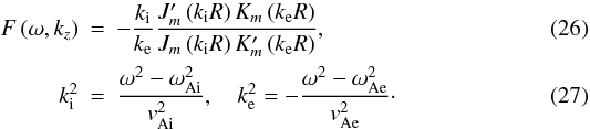 The
function F depends both on frequency ω and wave
number kz, taking that the tube has a
finite width into account. Note that F ≡ 1 in the limit of a TT (the
Bessel functions are approximated by their small arguments expressions), and we recover
the dispersion relation given by Eq. (1).
For a standing wave, kz is fixed and
Eq. (25) is solved for
ω, while for a propagating wave, ω is fixed and
Eq. (25) is solved for
kz. The solution to Eq. (25) corresponds again to the undamped kink
wave. For a finite width tube the analytical solution to this equation would imply to use
of additional terms in the asymptotic expansions of the Bessel functions, complicating
matters. We simply solve Eq. (25)
numerically in order to avoid these cumbersome calculations.
The
function F depends both on frequency ω and wave
number kz, taking that the tube has a
finite width into account. Note that F ≡ 1 in the limit of a TT (the
Bessel functions are approximated by their small arguments expressions), and we recover
the dispersion relation given by Eq. (1).
For a standing wave, kz is fixed and
Eq. (25) is solved for
ω, while for a propagating wave, ω is fixed and
Eq. (25) is solved for
kz. The solution to Eq. (25) corresponds again to the undamped kink
wave. For a finite width tube the analytical solution to this equation would imply to use
of additional terms in the asymptotic expansions of the Bessel functions, complicating
matters. We simply solve Eq. (25)
numerically in order to avoid these cumbersome calculations.
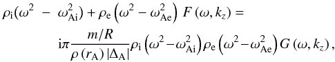
4.2. Inhomogeneous magnetic cylinder
When we add a thin non-uniform layer we obtain the complex dispersion relation
 (28)where
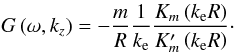 (29)For the TT we can again
use the asymptotic expansions of the Bessel function so that G ≡ 1, hence
in the TT limit, Eq. (28) is simplified to
Eq. (6). Equation (28) can be solved for a complex frequency
ω with a specified real wavenumber k∗ or
for a complex wavenumber kz for a specified
real frequency ω∗. By solving Eq. (28) in the case of a propagating wave with
real frequency ω∗ we find that the real part of
complex kz is
k∗ (we get again Eq. (25), k∗ is now different from Eq. (6)), while the imaginary part is given by
(29)For the TT we can again
use the asymptotic expansions of the Bessel function so that G ≡ 1, hence
in the TT limit, Eq. (28) is simplified to
Eq. (6). Equation (28) can be solved for a complex frequency
ω with a specified real wavenumber k∗ or
for a complex wavenumber kz for a specified
real frequency ω∗. By solving Eq. (28) in the case of a propagating wave with
real frequency ω∗ we find that the real part of
complex kz is
k∗ (we get again Eq. (25), k∗ is now different from Eq. (6)), while the imaginary part is given by
 (30)where
 ![Mathematical equation: \begin{eqnarray} \label{a} T &=& \frac{\pi}{2} \frac{m}{R} \frac{\left(\rho_{\mathrm i} - \rho_{\mathrm e}\right)^2}{\left[\rho_{\mathrm i} + \rho_{\mathrm e}F\left(\omega_*, k_*\right)\right]\left[1 + F\left(\omega_*, k_*\right)\right]^2}\nonumber \\[1.5mm] && \times\frac{F\left(\omega_*, k_*\right)\,G\left(\omega_*,k_*\right)}{ |{\rm d} \rho/{\rm d}r |_{r_{\mathrm A}}}, \end{eqnarray}](/articles/aa/full_html/2010/16/aa14845-10/aa14845-10-eq101.png) (31)and
(31)and
![Mathematical equation: \begin{equation} \label{b} N = 1 + \frac{k_*}{2} \frac{\rho_{\mathrm i} - \rho_{\mathrm e}}{\left[\rho_{\mathrm i} + \rho_{\mathrm e}F\left(\omega_*, k_*\right)\right]\left[1 + F\left(\omega_*,k_*\right)\right]} \left.\frac{\partial F}{\partial k}\right|_{\left(\omega_*, k_*\right)}\cdot \end{equation}](/articles/aa/full_html/2010/16/aa14845-10/aa14845-10-eq102.png) (32)The expressions are
slightly more complicated than in the TT approximation (see Eq. (10)), but
once k∗ is known the different terms can be easily
calculated. The corresponding damping per wavelength is
(32)The expressions are
slightly more complicated than in the TT approximation (see Eq. (10)), but
once k∗ is known the different terms can be easily
calculated. The corresponding damping per wavelength is  (33)In the TT limit,
i.e., when
F(ω∗,k∗)
and
G(ω∗,k∗) → 1
and ∂F/∂k → 0, we recover Eq. (11). For a sinusoidal density profile we
simply have to make use of Eq. (12)
in (31). Now let us define
(33)In the TT limit,
i.e., when
F(ω∗,k∗)
and
G(ω∗,k∗) → 1
and ∂F/∂k → 0, we recover Eq. (11). For a sinusoidal density profile we
simply have to make use of Eq. (12)
in (31). Now let us define
![Mathematical equation: \begin{equation} \widetilde{N} = 1-\frac{\omega_*}{2}\frac{\rho_{\mathrm i} - \rho_{\mathrm e}}{\left[\rho_{\mathrm i} + \rho_{\mathrm e}F\left(\omega_*, k_*\right)\right]\left[1 + F\left(\omega_*, k_*\right)\right]} \left.\frac{\partial F}{\partial \omega}\right|_{\left(\omega_*, k_*\right)}\cdot \end{equation}](/articles/aa/full_html/2010/16/aa14845-10/aa14845-10-eq107.png) (34)As in the previous
section, we compared, the damping per wavelength for propagating waves with the damping
per period, which in the non-TT approximation is given by
(34)As in the previous
section, we compared, the damping per wavelength for propagating waves with the damping
per period, which in the non-TT approximation is given by  (35)By
Eqs. (33) and (35), there is a clear correspondence between
the temporal and the spatial damping beyond the TT approximation. Furthermore, a general
expression that relates the temporal damping of standing waves and the spatial damping of
propagating waves can be derived following the analysis of Appendix A in Tagger et al. (1995). We can write the complex
dispersion relation given by Eq. (28) as
(35)By
Eqs. (33) and (35), there is a clear correspondence between
the temporal and the spatial damping beyond the TT approximation. Furthermore, a general
expression that relates the temporal damping of standing waves and the spatial damping of
propagating waves can be derived following the analysis of Appendix A in Tagger et al. (1995). We can write the complex
dispersion relation given by Eq. (28) as
 (36)To make it
clear, in Eq. (36),
DR is equal to the LHS of Eq. (28) and DI equal to minus the RHS of the
equation. In the case of spatial damping, if ω∗ and
k∗ are the solutions of
DR(ω,k) = 0 then it is easy to see by
making a Taylor expansion around the solution that
(36)To make it
clear, in Eq. (36),
DR is equal to the LHS of Eq. (28) and DI equal to minus the RHS of the
equation. In the case of spatial damping, if ω∗ and
k∗ are the solutions of
DR(ω,k) = 0 then it is easy to see by
making a Taylor expansion around the solution that  (37)while for
temporal damping
(37)while for
temporal damping  (38)Combining these
two expressions we find that
(38)Combining these
two expressions we find that  (39)which is simply
(see also Pascoe et al. 2010)
(39)which is simply
(see also Pascoe et al. 2010)  (40)This result is
valid when the damping is not too strong (see e.g., Tagger
et al. 1995), an assumption that we have already made in deriving the damping per
wavelength (kI ≪ kR). In the TT
approximation, kink waves are weakly dispersive so that
vgr ≈ vph in agreement with the
results found in Sect. 3, the damping per wavelength
is thus exactly the same as the damping per period, but in the regime when the TT
approximation is not applicable, the group speed can differ from the phase speed.
(40)This result is
valid when the damping is not too strong (see e.g., Tagger
et al. 1995), an assumption that we have already made in deriving the damping per
wavelength (kI ≪ kR). In the TT
approximation, kink waves are weakly dispersive so that
vgr ≈ vph in agreement with the
results found in Sect. 3, the damping per wavelength
is thus exactly the same as the damping per period, but in the regime when the TT
approximation is not applicable, the group speed can differ from the phase speed.
From the previous results, we can also derive alternative formulae for the damping per
wavelength and damping per period in terms of the imaginary part of the dispersion
relation, ![Mathematical equation: \begin{eqnarray} \frac{L_{\mathrm D}}{\lambda} &=& \frac{k_*}{2\pi}\frac{1}{D_{\mathrm I}\left(\omega_*, k_*\right)} \bigg\{-2 k_*\big[\rho_{\mathrm i}v^2_{\mathrm {Ai}}+ \rho_{\mathrm e}v^2_{\mathrm {Ae}} F\left(\omega_*,k_*\right)\big]\nonumber \\ & & + \rho_{\mathrm e}\left(\omega_*^2\!-\!k^2_*v^2_{\mathrm {Ae}}\right)\left.\frac{\partial F}{\partial k}\right|_{\left(\omega_*,k_*\right)}\bigg\}, \nonumber\\ \\ \frac{\tau_{\mathrm D}}{P} &=& \frac{\omega_*}{2\pi}\frac{1}{D_{\mathrm I}\left(\omega_*, k_*\right)}\nonumber \\ & & \times\left\{2 \omega_*\left[\rho_{\mathrm i}+\rho_{\mathrm e} F\left(\omega_*,k_*\right)\right] + \rho_{\mathrm e}\left(\omega_*^2\!-\!k^2_*v^2_{\mathrm {Ae}}\right)\left.\frac{\partial F}{\partial \omega}\right|_{\left(\omega_*,k_*\right)}\right\}\cdot \nonumber\\ \end{eqnarray}](/articles/aa/full_html/2010/16/aa14845-10/aa14845-10-eq119.png) Using
Eq. (40) we can identify in these
expressions the terms related to the phase and group speed.
Using
Eq. (40) we can identify in these
expressions the terms related to the phase and group speed.
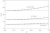 |
Fig. 1 Damping per wavelength as a function of the dimensionless frequency (f = ωR/vAi) for three different widths of the inhomogeneous layers. The solid line corresponds to the analytical results, and the dashed line represents the full numerical solution of the resistive eigenvalue problem. The dotted line corresponds to the TT approximation, valid when f → 0. In this plot ρi/ρe = 3. |
Next using the analytical results given in this section, we study how the damping per
wavelength depends on the dimensionless frequency of the driver f,
defined by Eq. (23), for particular cases
(see Fig. 1). We see that the wider the layer, the
more efficient the attenuation (smaller damping per wavelengths), in agreement with the
analytical results in the TT approximation. For small f the damping per
wavelength tends to the TT value. The value of
LD/λ increases monotonically with
ω. The deviation with respect to the TT results is smaller for thick
layers. In the TT approximation, which for propagating waves, is the low-frequency
approximation, LD/λ is independent of
frequency, since this approximation does not take into account the variation of frequency;
i.e., the frequency is only presumed to be low. The analytical results for
LD/λ beyond the TT approximation, take
the dependence on frequency into account. The value of
LD/λ now undergoes a moderate increase
when we move from low to high frequencies. However, the really interesting quantity to
calculate is the damping length itself. To make the dependence of
LD on frequency more explicit, we follow the same line of
reasoning in Sect. 3.2 and rewrite Eq. (13) as
 (43)where the quantity
ξEW now depends on the parameters of the equilibrium model
and the characteristics of the wave itself. Again
λ = 2π/kz
and kz is related to the frequency by the
dispersion relation Eq. (25). Since we
have abandoned the TT approximation, a simple analytical formula that
relates kz to ω is not
readily available, but we can always write
(43)where the quantity
ξEW now depends on the parameters of the equilibrium model
and the characteristics of the wave itself. Again
λ = 2π/kz
and kz is related to the frequency by the
dispersion relation Eq. (25). Since we
have abandoned the TT approximation, a simple analytical formula that
relates kz to ω is not
readily available, but we can always write
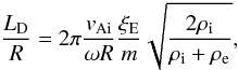
 (44)where f
is the dimensionless frequency defined in Eq. (23), and ψ(f) is a function that we can
determine numerically. As a result by implementing the
function ψ(f), we find that
(44)where f
is the dimensionless frequency defined in Eq. (23), and ψ(f) is a function that we can
determine numerically. As a result by implementing the
function ψ(f), we find that  (45)which in the
low-frequency limit is equivalent to the TGV relation given by Eq. (24) for m = 1; i.e.,
(45)which in the
low-frequency limit is equivalent to the TGV relation given by Eq. (24) for m = 1; i.e.,
 (46)as
f → 0, where ξE is defined by Eq. (17). In Eq. (45) since ψ(f) and
ξEW are slowly varying functions of f, the
main dependence of LD on f is contained in
the factor 1/f, as in the low-frequency limit shown by Eq. (24). This is illustrated in Fig. 2, where
LD/R is plotted as a function
of f for several values of l/R. The
dependence of the curves on 1/f is very clear, and the non-TT and TT
solutions tend to overlap in the limit of f → 0, where both cases are
accurately described by the TGV relation. Even for f → 1 the TGV relation
still describes the behaviour of the damping length with frequency quite well. Again, the
potential of resonant absorption as a frequency filter is clearly demonstrated in
Fig. 2, with high-frequency waves being damped on
shorter spatial scales than low-frequency waves (for
fixed l/R).
(46)as
f → 0, where ξE is defined by Eq. (17). In Eq. (45) since ψ(f) and
ξEW are slowly varying functions of f, the
main dependence of LD on f is contained in
the factor 1/f, as in the low-frequency limit shown by Eq. (24). This is illustrated in Fig. 2, where
LD/R is plotted as a function
of f for several values of l/R. The
dependence of the curves on 1/f is very clear, and the non-TT and TT
solutions tend to overlap in the limit of f → 0, where both cases are
accurately described by the TGV relation. Even for f → 1 the TGV relation
still describes the behaviour of the damping length with frequency quite well. Again, the
potential of resonant absorption as a frequency filter is clearly demonstrated in
Fig. 2, with high-frequency waves being damped on
shorter spatial scales than low-frequency waves (for
fixed l/R).
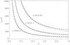 |
Fig. 2 Damping length normalised to the loop radius as a function of the dimensionless frequency (f = ωR/vAi) for three different widths of the inhomogeneous layers. The solid line corresponds to the analytical results, the dashed line represents the full numerical solution of the resistive eigenvalue problem, and the dotted line corresponds to the TT approximation calculated using Eq. (24), valid when f → 0. In this plot ρi/ρe = 3. |
5. Resistive calculations
The results based on TB approximation described in the previous sections are compared with the full resistive calculations using the same cylindrical tube model. The same approach as in Terradas et al. (2006) is used: i.e., the linearised MHD equations including magnetic diffusion are numerically solved using finite elements. This method allows us to calculate the complex eigenfrequencies of the quasimodes, which are independent of the value of the resistivity in the limit of large resistivity (see Poedts & Kerner 1991).
The comparison with the analytical results is useful since there are no implicit assumptions about the TT or TB approximation in the resistive eigenvalue problem; i.e., the TT and TB approximations are not used. The resistive calculation applies to any frequency, whether it is small compared to vAi/R or not, and also to equilibrium models that have a thin non-uniform layer or are fully non-uniform. We have solved the eigenvalue problem (for ω) and have used Eq. (40) to translate from temporal damping to spatial damping. By including resistivity, the eigenvalue problem for the wavenumber is more difficult to solve than the eigenvalue problem for the frequency. The results of the resistive calculations are shown in Figs. 1 and 2 where the damping per wavelength and the damping length are plotted as a function of the frequency of the driver. The agreement between the resistive computations and the analytical or semi-analytical methods is very good. The small differences are the result of assuming that the resonance is always located at r = R in the analytical approximations, and we have calculated the derivative of the density at this position. This explains the small deviations from the resistive estimations. A more precise determination could be done by calculating the exact location of the resonance and then using a slightly modified version of Eq. (28), but since the analytical approximations that we have already derived are quite satisfactory, there is no pressing need to explore this further.
6. Conclusions and discussion
The spatial damping due to resonant absorption of driven kink waves has been investigated. The main conclusion of the work is that the damping length of propagating kink waves due to resonant absorption is a monotonically decreasing function of frequency. The TGV relation for kink waves was derived, demonstrating that for low frequencies the damping length is exactly inversely proportional to frequency. In the high-frequency range the TGV relation continues to be an excellent approximation of the actual dependency of the damping length on frequency. Certainly, for all physically relevant frequencies the dependency of damping length on frequency is accurately described by the TGV relation. This dependency means that resonant absorption is selective as it favours low-frequency waves and can efficiently remove high-frequency waves from a broad band spectrum of kink waves. This has high significance for solar atmospheric kink waves, since high-frequency waves will tend to lose more power than their low-frequency counterparts before reaching high altitudes in the solar corona, with the exact percentage power loss depending on the properties of the equilibrium, in particular the width of the non-uniform layer and steepness of the variation in the local Alfvén speed. With respect to mode conversion, the process of resonant absorption will cause the higher frequency waves to be attenuated more because the global kink mode will be converted into localised Alfvénic modes at lower heights. If the energy of these Alfvénic motions is eventually dissipated, then resonant absorption should produce a characteristic distribution of the energy as a function of height in the solar atmosphere. This could have important consequences with for the spatial distribution of wave heating in the solar atmosphere.
It has also been shown that spatial and temporal damping are basically equivalent. In the TT approximation, the damping per period and the damping per wavelength are exactly the same. The differences in these two quantities arise in the regime where the TT is not valid, but even in this situation it is easy to relate the spatial and the temporal damping rates through the group and phase speeds of the kink MHD waves. This allows us to translate the results from the temporally damped waves (ω complex, k real) to spatially attenuated waves (ω real, k complex) due to resonant absorption. This mechanism requires the frequency of the driver to be between the internal and the external Alfvén frequency of the tube. This might seem a very restrictive condition, but in fact it is just the opposite. In the driven problem, the frequency is fixed but the system chooses the proper wavelength (along the waveguide) to accommodate the kink mode in the tube. This kink mode generated at the base of the loop propagates upwards along the tube and at the same time is attenuated by the inhomogeneity at the tube boundary.
An interesting result is that both the damping length in the spatial problem and the damping time in the temporal problem are always smaller than in the TT approximation (when f → 0), meaning that waves with short wavelengths or high frequencies are always more efficiently damped. The observations of standing kink waves observed with TRACE and for the propagating kink waves detected with the CoMP instrument are precisely in the regime where the TT is applicable, i.e., where the waves are less affected by resonant absorption. That overtones of standing kink waves and high-frequency propagating waves have proved difficult to detect may be a direct consequence of the filtering by resonant absorption. From a different perspective, we have also shown that the damping per wavelength (and the damping per period) has a weak dependence on the frequency.
It is necessary to point out that our results are based on a simple magnetic flux tube model, i.e., a straight cylinder, with no gravity and pressure. Curvature might produce some damping due to wave leakage and external resonances, while stratification might be important if the wavelength of the propagating kink modes is less than the typical density scale height of the solar corona. The effect of gas pressure should be small since the corona is expected to have very small beta. These issues need to be investigated in the future. The only inhomogeneity in our model is plasma density in the radial direction; however, this is a characteristic property of solar waveguides that is observed at all atmospheric heights, e.g., chromospheric magnetic bright points or coronal loops. Thus the theory of resonant damping of propagating kink waves due to radial plasma density inhomogeneity offers a natural explanation for the dissipation observed by, e.g., Tomczyk & McIntosh (2009). However, a detailed comparison between the observations and the expected frequency-dependent response by resonant absorption is needed to quantify the precise spatial distribution of wave heating because this mechanism in the solar plasma, e.g., kink wave dissipation as a function of both frequency and height. This problem is addressed in Verth et al. (2010).
Acknowledgments
J.T. acknowledges the Universitat de les Illes Balears for a postdoctoral position and the funding provided under projects AYA2006-07637 (Spanish Ministerio de Educación y Ciencia). M.G. and G.V. acknowledge support from K. U. Leuven via GOA/2009-009. The authors thank the anonymous referee for useful comments that helped to improve the paper.
References
- Andries, J., Arregui, I., & Goossens, M. 2005a, ApJ, 624, L57 [NASA ADS] [CrossRef] [Google Scholar]
- Andries, J., Goossens, M., Hollweg, J. V., Arregui, I., & Van Doorsselaere, T. 2005b, A&A, 430, 1109 [NASA ADS] [CrossRef] [EDP Sciences] [Google Scholar]
- Arregui, I., & Ballester, J. L. 2010, Space Sci. Rev., accepted [arXiv:1002.3489] [Google Scholar]
- Arregui, I., Van Doorsselaere, T., Andries, J., Goossens, M., & Kimpe, D. 2005, A&A, 441, 361 [NASA ADS] [CrossRef] [EDP Sciences] [Google Scholar]
- Arregui, I., Andries, J., Van Doorsselaere, T., Goossens, M., & Poedts, S. 2007, A&A, 463, 333 [NASA ADS] [CrossRef] [EDP Sciences] [Google Scholar]
- Arregui, I., Terradas, J., Oliver, R., & Ballester, J. L. 2008, ApJ, 682, L141 [NASA ADS] [CrossRef] [Google Scholar]
- Aschwanden, M. J. 2005, ApJ, 634, L193 [NASA ADS] [CrossRef] [Google Scholar]
- Aschwanden, M. J., Fletcher, L., Schrijver, C. J., & Alexander, D. 1999, ApJ, 520, 880 [NASA ADS] [CrossRef] [Google Scholar]
- Aschwanden, M. J., de Pontieu, B., Schrijver, C. J., & Title, A. M. 2002, Sol. Phys., 206, 99 [NASA ADS] [CrossRef] [Google Scholar]
- Aschwanden, M. J., Nightingale, R. W., Andries, J., Goossens, M., & Van Doorsselaere, T. 2003, ApJ, 598, 1375 [NASA ADS] [CrossRef] [Google Scholar]
- Berghmans, D., & de Bruyne, P. 1995, ApJ, 453, 495 [NASA ADS] [CrossRef] [Google Scholar]
- Brady, C. S., & Arber, T. D. 2005, A&A, 438, 733 [NASA ADS] [CrossRef] [EDP Sciences] [Google Scholar]
- De Moortel, I., & Brady, C. S. 2007, ApJ, 664, 1210 [NASA ADS] [CrossRef] [Google Scholar]
- De Pontieu, B., Martens, P. C. H., & Hudson, H. S. 2001, ApJ, 558, 859 [NASA ADS] [CrossRef] [Google Scholar]
- De Pontieu, B., McIntosh, S. W., Carlsson, M., et al. 2007, Science, 318, 1574 [NASA ADS] [CrossRef] [PubMed] [Google Scholar]
- Díaz, A. J., Oliver, R., Ballester, J. L., & Roberts, B. 2004, A&A, 424, 1055 [NASA ADS] [CrossRef] [EDP Sciences] [Google Scholar]
- Dymova, M. V., & Ruderman, M. S. 2006, A&A, 457, 1059 [NASA ADS] [CrossRef] [EDP Sciences] [Google Scholar]
- Edwin, P. M., & Roberts, B. 1983, Sol. Phys., 88, 179 [NASA ADS] [CrossRef] [Google Scholar]
- Erdélyi, R., & Verth, G. 2007, A&A, 462, 743 [NASA ADS] [CrossRef] [EDP Sciences] [Google Scholar]
- Fujimura, D., & Tsuneta, S. 2009, ApJ, 702, 1443 [NASA ADS] [CrossRef] [Google Scholar]
- Goossens, M. 2008, in IAU Symp., 247, 228 [Google Scholar]
- Goossens, M., Hollweg, J. V., & Sakurai, T. 1992, Sol. Phys., 138, 233 [NASA ADS] [CrossRef] [Google Scholar]
- Goossens, M., Ruderman, M. S., & Hollweg, J. V. 1995, Sol. Phys., 157, 75 [NASA ADS] [CrossRef] [Google Scholar]
- Goossens, M., Andries, J., & Aschwanden, M. J. 2002, A&A, 394, L39 [NASA ADS] [CrossRef] [EDP Sciences] [Google Scholar]
- Goossens, M., Andries, J., & Arregui, I. 2006, Royal Soc. London Philos. Trans. Ser. A, 364, 433 [Google Scholar]
- Goossens, M., Arregui, I., Ballester, J. L., & Wang, T. J. 2008, A&A, 484, 851 [NASA ADS] [CrossRef] [EDP Sciences] [Google Scholar]
- Goossens, M., Terradas, J., Andries, J., Arregui, I., & Ballester, J. L. 2009, A&A, 503, 213 [NASA ADS] [CrossRef] [EDP Sciences] [Google Scholar]
- He, J., Tu, C., Marsch, E., et al. 2009, A&A, 497, 525 [NASA ADS] [CrossRef] [EDP Sciences] [Google Scholar]
- Heyvaerts, J., & Priest, E. R. 1983, A&A, 117, 220 [NASA ADS] [Google Scholar]
- Hollweg, J. V., & Yang, G. 1988, J. Geophys. Res., 93, 5423 [NASA ADS] [CrossRef] [Google Scholar]
- Ionson, J. A. 1978, ApJ, 226, 650 [NASA ADS] [CrossRef] [Google Scholar]
- Jess, D. B., Mathioudakis, M., Erdélyi, R., et al. 2009, Science, 323, 1582 [NASA ADS] [CrossRef] [PubMed] [Google Scholar]
- Lin, Y., Soler, R., Engvold, O., et al. 2009, ApJ, 704, 870 [NASA ADS] [CrossRef] [Google Scholar]
- McLaughlin, J. A., & Ofman, L. 2008, ApJ, 682, 1338 [NASA ADS] [CrossRef] [Google Scholar]
- Morton, R. J., & Erdélyi, R. 2009, ApJ, 707, 750 [NASA ADS] [CrossRef] [Google Scholar]
- Nakariakov, V. M., Ofman, L., Deluca, E. E., Roberts, B., & Davila, J. M. 1999, Science, 285, 862 [NASA ADS] [CrossRef] [PubMed] [Google Scholar]
- Ofman, L. 2005, Adv. Space Res., 36, 1572 [NASA ADS] [CrossRef] [Google Scholar]
- Ofman, L., & Aschwanden, M. J. 2002, ApJ, 576, L153 [NASA ADS] [CrossRef] [Google Scholar]
- Ofman, L., & Davila, J. M. 1995, J. Geophys. Res., 100, 23427 [NASA ADS] [CrossRef] [Google Scholar]
- Okamoto, T. J., Tsuneta, S., Berger, T. E., et al. 2007, Science, 318, 1577 [NASA ADS] [CrossRef] [PubMed] [Google Scholar]
- Pascoe, D. J., Wright, A. N., & De Moortel, I. 2010, ApJ, 711, 990 [NASA ADS] [CrossRef] [Google Scholar]
- Poedts, S., & Kerner, W. 1991, Phys. Rev. Lett., 66, 2871 [NASA ADS] [CrossRef] [PubMed] [Google Scholar]
- Roberts, B. 2002, in Solar Variability: From Core to Outer Frontiers, ed. A. Wilson, ESA SP, 506, 481 [NASA ADS] [Google Scholar]
- Roberts, B., Edwin, P. M., & Benz, A. O. 1984, ApJ, 279, 857 [NASA ADS] [CrossRef] [Google Scholar]
- Ruderman, M. S., & Erdélyi, R. 2009, Space Sci. Rev., 149, 199 [NASA ADS] [CrossRef] [Google Scholar]
- Ruderman, M. S., & Roberts, B. 2002, ApJ, 577, 475 [NASA ADS] [CrossRef] [Google Scholar]
- Ruderman, M. S., Verth, G., & Erdélyi, R. 2008, ApJ, 686, 694 [NASA ADS] [CrossRef] [Google Scholar]
- Sakurai, T., Goossens, M., & Hollweg, J. V. 1991, Sol. Phys., 133, 227 [NASA ADS] [CrossRef] [Google Scholar]
- Selwa, M., Murawski, K., Solanki, S. K., Wang, T. J., & Tóth, G. 2005, A&A, 440, 385 [NASA ADS] [CrossRef] [EDP Sciences] [Google Scholar]
- Selwa, M., Murawski, K., Solanki, S. K., & Wang, T. J. 2007, A&A, 462, 1127 [NASA ADS] [CrossRef] [EDP Sciences] [Google Scholar]
- Smith, J. M., Roberts, B., & Oliver, R. 1997, A&A, 317, 752 [NASA ADS] [Google Scholar]
- Soler, R., Oliver, R., & Ballester, J. L. 2009a, ApJ, 707, 662 [NASA ADS] [CrossRef] [Google Scholar]
- Soler, R., Oliver, R., Ballester, J. L., & Goossens, M. 2009b, ApJ, 695, L166 [NASA ADS] [CrossRef] [Google Scholar]
- Steinolfson, R. S., & Davila, J. M. 1993, ApJ, 415, 354 [NASA ADS] [CrossRef] [Google Scholar]
- Tagger, M., Falgarone, E., & Shukurov, A. 1995, A&A, 299, 940 [NASA ADS] [Google Scholar]
- Terradas, J. 2009, Space Sci. Rev., 149, 255 [NASA ADS] [CrossRef] [Google Scholar]
- Terradas, J., Oliver, R., & Ballester, J. L. 2006, ApJ, 642, 533 [NASA ADS] [CrossRef] [Google Scholar]
- Terradas, J., Arregui, I., Oliver, R., et al. 2008, ApJ, 679, 1611 [NASA ADS] [CrossRef] [Google Scholar]
- Tirry, W. J., & Goossens, M. 1996, ApJ, 471, 501 [NASA ADS] [CrossRef] [Google Scholar]
- Tirry, W. J., Berghmans, D., & Goossens, M. 1997, A&A, 322, 329 [NASA ADS] [Google Scholar]
- Tirry, W. J., Cadez, V. M., Erdélyi, R., & Goossens, M. 1998, A&A, 332, 786 [NASA ADS] [Google Scholar]
- Tomczyk, S., & McIntosh, S. W. 2009, ApJ, 697, 1384 [NASA ADS] [CrossRef] [Google Scholar]
- Tomczyk, S., McIntosh, S. W., Keil, S. L., et al. 2007, Science, 317, 1192 [NASA ADS] [CrossRef] [PubMed] [Google Scholar]
- Uchida, Y. 1970, PASJ, 22, 341 [NASA ADS] [Google Scholar]
- Van Doorsselaere, T., Brady, C. S., Verwichte, E., & Nakariakov, V. M. 2008, A&A, 491, L9 [NASA ADS] [CrossRef] [EDP Sciences] [Google Scholar]
- Van Doorsselaere, T., Birtill, D. C. C., & Evans, G. R. 2009, A&A, 508, 1485 [NASA ADS] [CrossRef] [EDP Sciences] [Google Scholar]
- Vasheghani Farahani, S., Van Doorsselaere, T., Verwichte, E., & Nakariakov, V. M. 2009, A&A, 498, L29 [NASA ADS] [CrossRef] [EDP Sciences] [Google Scholar]
- Verth, G., & Erdélyi, R. 2008, A&A, 486, 1015 [NASA ADS] [CrossRef] [EDP Sciences] [Google Scholar]
- Verth, G., Van Doorsselaere, T., Erdélyi, R., & Goossens, M. 2007, A&A, 475, 341 [NASA ADS] [CrossRef] [EDP Sciences] [Google Scholar]
- Verth, G., Erdélyi, R., & Jess, D. B. 2008, ApJ, 687, L45 [NASA ADS] [CrossRef] [Google Scholar]
- Verth, G., Terradas, J., & Goossens, M. 2010, ApJ, 718, L102 [NASA ADS] [CrossRef] [Google Scholar]
- Verwichte, E., Nakariakov, V. M., Ofman, L., & Deluca, E. E. 2004, Sol. Phys., 223, 77 [NASA ADS] [CrossRef] [Google Scholar]
- Verwichte, E., Foullon, C., & Nakariakov, V. M. 2006, A&A, 446, 1139 [NASA ADS] [CrossRef] [EDP Sciences] [Google Scholar]
All Tables
Estimated range of kzR in observed propagating (P) and standing (S) MHD wave modes.
All Figures
|
Fig. 1 Damping per wavelength as a function of the dimensionless frequency (f = ωR/vAi) for three different widths of the inhomogeneous layers. The solid line corresponds to the analytical results, and the dashed line represents the full numerical solution of the resistive eigenvalue problem. The dotted line corresponds to the TT approximation, valid when f → 0. In this plot ρi/ρe = 3. |
| In the text | |
|
Fig. 2 Damping length normalised to the loop radius as a function of the dimensionless frequency (f = ωR/vAi) for three different widths of the inhomogeneous layers. The solid line corresponds to the analytical results, the dashed line represents the full numerical solution of the resistive eigenvalue problem, and the dotted line corresponds to the TT approximation calculated using Eq. (24), valid when f → 0. In this plot ρi/ρe = 3. |
| In the text | |
Current usage metrics show cumulative count of Article Views (full-text article views including HTML views, PDF and ePub downloads, according to the available data) and Abstracts Views on Vision4Press platform.
Data correspond to usage on the plateform after 2015. The current usage metrics is available 48-96 hours after online publication and is updated daily on week days.
Initial download of the metrics may take a while.