| Issue |
A&A
Volume 524, December 2010
|
|
|---|---|---|
| Article Number | A87 | |
| Number of page(s) | 5 | |
| Section | Stellar structure and evolution | |
| DOI | https://doi.org/10.1051/0004-6361/201014514 | |
| Published online | 25 November 2010 | |
Bolometric corrections for cool giants based on near-infrared photometry
1
University of ViennaDepartment of Astronomy,
Türkenschanzstraße 17,
1180
Vienna,
Austria
e-mail: franz.kerschbaum@univie.ac.at
2
Association Austria Solar, Mariahilferstrasse 89/22,
1060
Vienna,
Austria
Received: 26 March 2010
Accepted: 30 September 2010
Context. The bolometric luminosity is one of the most fundamental stellar parameters that is generally not directly observable. When integrating whole spectral energy distributions, bolometric corrections are widely used. These corrections are typically specified for a well defined object type, a measured photometric colour, and the colour index range for which it is calibrated.
Aims. We provide this bolometric correction for the near-infrared colours of red late giants.
Methods. We compare bolometric luminosities derived from fits to spectral energy distributions covering the visual and near, mid, and far infrared to different near-infrared colour indices to define subgroups within our stellar sample and finally obtain specific bolometric corrections.
Results. For well-defined subgroups of different near-infrared colours and atmospheric chemistry, we present four distinct bolometric colour relations and compare these to earlier results from the literature.
Key words: stars: late-type / stars: AGB and post-AGB / stars: carbon / stars: fundamental parameters / infrared: stars
© ESO, 2010
1. Introduction
Deriving bolometric luminosities from the photometric measurements of a star in various bands is a key stage in the comparison of stellar model predictions with observations. In the field of cool giants, the determination of the bolometric correction remains a challenging task. In these objects, millions of molecular lines – with their relatively high sensitivity to stellar structure and parameters – strongly affect the stellar flux. In addition, it remains to describe the transfer of part of the stellar flux into the mid- and far-infrared range by circumstellar dust that occurs because of enhanced mass loss during the asymptotic giant branch (AGB) phase. This process is indeed barely taken into account in previous studies that attempt to provide relations for the bolometric correction of a star’s colour.
We begin with a brief summary of the literature published in this area and focus thereby on relations for BCK versus (vs.) (J − K). A first detailed study of the bolometric correction for very cool giants was presented by Bessell & Wood (1984), who also discuss a few earlier attempts. They pointed out the usefulness of searching for a relation in the near infrared for this kind of stars. Bessell et al. (1998) provided a relation for (V − K) vs. BCK derived from model spectra down to Teff = 3600 K. In the same year, Montegriffo et al. (1998) published a set of bolometric corrections derived from black-body fits to population II stars. Their data extend down to Teff = 3200 K (below which their theoretical and empirical temperature scale strongly diverge) or (J − K) = 1.3. Costa & Frogel (1996) published a formula for the bolometric correction of carbon stars in the LMC, covering in (J − K) a range from 1 to 2.6. Another formula for carbon stars is given in Whitelock et al. (2006). The formula of Costa & Frogel is in good agreement with dust-free models of carbon stars presented by Aringer et al. (2009), while the Whitelock relation seems to represent stars with a higher mass-loss rate. Houdashelt et al. (2000) tackled again the problem from the perspective of stellar models (calibrated from observations) and gave BCK values for giants down to Teff = 4000 K or (J − K) = 0.95 for various metallicities. The most recent work in this area was presented by Guandalini & Busso (2008), who also extended the investigated range to lower temperatures. Their sample is focused on stars of spectral type MS and S, and they derive bolometric corrections for the colours (K − [8.8]) and (K − [12.5]).
In this paper, we present another approach on calculating the bolometric correction for cool, highly extended and partly dusty AGB stars using a large sample of field AGB stars covering a range in (J − K) between 1 and 2.9 mag.
2. Data base
The starting point of our analysis was a database of black-body fits to the spectral energy distribution (SED) of a sample of 832 long-period variables (Kerschbaum & Hron 1996; Kerschbaum 1999). For the fits, the SED was traced by J, H, K, and L′ band photometry (Kerschbaum & Hron 1994; Kerschbaum 1995, and references therein), visual data from the General Catalogue of Variable Stars (Kholopov et al. 1985 − 88), and mid- and far-infrared photometry from the IRAS Point Source Catalogue (Joint IRAS Working Group 1988). For details, we refer to Kerschbaum & Hron (1996). From the resulting SEDs, Kerschbaum & Hron (1996) and Kerschbaum (1999) derived mbol values by fitting two black-bodies to the SEDs – one for the photospheric component and one for the dust shell. Where a good fit to the photometric data was achieved with only one black-body, a second black-body component was omitted (obviously dust-free stars). For two black-bodies, a ratio of the luminosity inferred from the two fits was calculated.
All objects in our sample are nearby field AGB stars. Information on the atmospheric and dust chemistry, i.e. oxygen rich or carbon rich, was available for all of these targets: our sample includes 146 C-stars, 655 M- or K-type stars and 31 objects of spectral class S. For the definition of the chemistry we used both the spectral type from the GCVS and information from IRAS. The largest fraction of stars in our sample are thus of spectral type M (i.e. O-rich), so we will put the main focus of our investigation on this group. From the GCVS we have also information on the variability sub-type of our long-period variables and find 230, 369, and 233 stars classified as irregular, semi-regular, and mira-like variables, respectively. Thus our sample represents a good coverage of the parameter range of LPVs in terms of chemistry and variability type. Since the number of S-type stars is so small, we do not investigate them further here.
3. Results
3.1. BCK vs. (J – K)
To find a reliable relation between near-infrared data and the bolometric luminosity, we started with a couple of tests to assess a possible division between the subgroups in our sample. As a first test we plotted in Fig. 1 the bolometric correction, defined as BCK = mbol − K, against (J − K), differentiating between O-rich (upper panel) and C-rich (lower panel) stars. The S-type stars were included in the lower panel.
We begin our analysis with the C-rich stars that present a rather clear picture: up to (J − K) = 2, BCK increases steadily with colour. The same trend is also seen for the S-type stars, but they may show a systematic offset of approximately 0.1 mag towards a higher BCK value. The S-type stars were not analysed further because of their low number in our sample. For C-stars redder than (J − K) = 2, the relation between colour and bolometric correction seems to be inverted. A 2nd order polynomial was fitted through all the C-stars resulting in the curve shown in Fig. 1 (lower panel). As a first formula for the bolometric correction, we thus derive for the C-stars the relation  (1)defined for J − K = 1.0 to 4.4. The standard deviation from this sequence is 0.11 mag over the whole range in J − K. As can be seen in Fig. 1, the scatter is smaller below J − K = 2 (σ = 0.06 mag) than above this colour value (σ = 0.15 mag). We note that Bessell & Wood (1984) also derived a second-order polynomial fit from their data set (O-rich and C-rich), while Costa & Frogel (1996) used a fourth-degree polynomial to fit their sample of C-stars. A comparison of these relations with our results is given below.
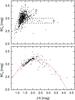 |
Fig. 1 Bolometric correction derived from black-body fits vs. (J − K). The upper panel shows the results for O-rich stars (spectral type M or K), while the lower panel presents the reuslts for the C-type stars (filled circles). S-type stars are also shown in the lower panel and are marked with crosses. See text for details. |
In the O-rich case (upper panel of Fig. 1), the situation is less clear. A simple polynomial fit would again be a helpful solution1. However, the distribution of the data points in the colour-BCK plane is clearly inconsistent with such a solution. The O-rich stars are numerous enough to look for possible substructure in the plane. As a starting point, we identify by eye three possible sequences, which we marked in Fig. 1 by numbers 1 to 3. These sequences correspond to slopes in the colour-BCK plane of 2, 0.5, and 0, respectively. While the colour range covered by each sequence is shifted towards the red from 1 to 3, there is considerable overlap between the sequences. For stars with J − K values in these overlap regions, an exact bolometric correction based on only one colour becomes impossible. This problem appears for most of the stars, because for (J − K) < 2.2 the (J − K) index is obviously insufficient to handle the influence of the circumstellar dust component correctly.
For stars with (J − K) > 2.2, all stars follow the sequence “3” and the bolometric correction is a constant value independent of colour. Thus, the K-magnitude there becomes an excellent indicator of mbol.
A closer inspection of the stars of sequence “3” indicates that their SED can only be fitted by a combination of two black-bodies. This implies that a detectable dust shell surrounds the star. Stars that could be fitted with only one black-body, i.e. dust-free stars, are all found close to sequence “1”. However, if we examine at the distribution of stars fitted with two black-bodies, we find them all over Fig. 1, upper panel. Thus, knowledge of an infrared excess alone is insufficient to derive a proper bolometric correction from (J − K).
From SED fitting, we inferred not only the number of black-bodies but also their luminosity ratio Ldust / Lstar (see Kerschbaum & Hron 1996). The larger the luminosity ratio, the more dust can be detected around the star, thus the stronger is the mass-loss. We divided our sample into three subgroups of luminosity ratios either below 0.013, between 0.013 and 0.025, or above 0.25, respectively. The 137 stars fitted with only one black-body were not taken into account for this step. The limit of 0.013 was chosen as it is the median value of all stars in our sample. The second division was chosen because above a luminosity ratio of 0.025 the stars have increasingly higher (J − K) values. The result of this exercise is presented in Fig. 2. While we see that stars with a higher luminosity ratio tend to exhibit a flatter (J − K) vs. BCK relation, a clear separation between the groups is not obvious. As a result, we must search for an additional parameter to achieve an accurate determination of the bolometric correction except for very red stars and stars with pure (dust free) photospheric colours (single black-body).
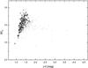 |
Fig. 2 The colour index J − K vs. the bolometric correction for the O-rich stars of our sample that required two black-bodies when fitting their SED. The sample is separated into three groups according to the luminosity ratio of the two black-bodies: L-ratio < 0.013 (filled circles), 0.013 ≤ L-ratio < 0.025 (open circles), and L-ratio ≤ 0.025 (crosses). |
3.2. Alternative relations
The next logical step was to identify an additional criterion to help us define more clearly various sequences in the (J − K) vs. BCK plane. We begin this search by including the type of variability, mira, semiregular or irregular variable, in our analysis. The classification was taken from the General Catalogue of Variable Stars. Supergiants (of variability type Lc or SRc) and stars with uncertain variability information were removed from our sample at this step. The outcome is presented in Fig. 3. From this figure, it is obvious that only miras are located on sequence “3”, but that they are also found on the other two sequences. The other two classes of variables overlap on sequences “1” and “2”. Accordingly, the variability type is also not a sufficient criterion for deriving a bolometric correction from (J − K).
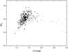 |
Fig. 3 The colour index (J − K) versus the bolometric correction for the O-rich stars of our sample separated according to their variability type: irregular variables (filled circles), semiregular variables (open circles), and miras (crosses). |
The remaining solution was to add observations acquired using additional filters to our analysis. Using (J − H) instead of (J − K) leads to an even larger scatter in the colour-BC relation. A good indicator of dust should result from a combination with mid-infrared photometry, but a test using (K − [12]) as a colour index lead to a similar indeterminacy for BCK.
These first tests show that a description focusing on either the dust or the photospheric component does not help us derive a reliable relation for the bolometric correction. Therefore we have to search for a combination of filters that allows us to describe the whole SED more properly. In this light, one has to be concerned that a combination of (J − H) and (H − K), i.e., the colours available for the largest number of cool giants in the 2MASS survey, is of little help. Our test, indeed indicates that any obvious segregation in the two-colour plane is not reflected in a clearer separation in the colour-BCK plane. The only exception is again group “3”.
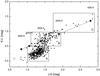 |
Fig. 4 Two-colour diagram (J − K) vs. (K − L′) for our sample stars, divided into three regions related to three different colour-mbol relations. See Fig. 5. The open circles give the intrinsic colours for giants of spectral type K0, K3, M1, and M5 from Bessell & Brett (1988), respectively. The large filled boxes mark the colours of black-body SEDs from 3500 to 1500 K. |
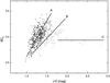 |
Fig. 5 The colour index (J − K) versus the bolometric correction for the O-rich stars of our sample separated according to their location in the (J − K) vs. (K − L′) two-colour diagram (see Fig. 4). |
For 568 O-rich stars of our sample, we also have access to measurements in the L′-band (centered on 3.8 μm). A two-colour diagram using (J − K) and (K − L′) was plotted and divided into three different regions named A, B, and C, respectively (Fig. 4). The starting point for the chosen division was to roughly separate the sequence observed in Fig. 4 into three equal parts in (K − L′), a step that was later refined to provide an optimum separation in the (J − K) vs. BCK plane as plotted in Fig. 5. As can be seen, the three groups A, B, and C hardly overlap in Fig. 5, suggesting that this selection criterion is indeed sufficient to derive a proper bolometric correction for the K-band filter from J, K, and L′ magnitudes. The remaining scatter can be easily explained by stellar variability. We fitted linear equations for the three groups and provide the results in Table 1 together with the chosen limits for the three groups in the two-colour diagram (Fig. 4). This, at the same time, delineates the valid (J − K) range for our relations. The final relations are also plotted in Fig. 5.
To more clearly understand the origin of the three groups in the (J − K) vs. (K − L′) plane, we added the corresponding colour values for a black-body (large filled boxes connected by a solid line) and the intrinsic colours for giants from Bessell & Brett (1988, large open circles) to Fig. 4. Stars in group “A”, obviously, are in good agreement with the colours given by Bessell & Brett and seem to extend their spectroscopic sequence beyond M5 (the last data point given by these authors). Around (J − K) = 1.3, the linear trend is no longer followed by the observations, and we instead see an increase in (K − L′) at a rather constant (J − K) until the data points reach the black-body sequence. For redder (J − K), the observations are reproduced well by a series of black-bodies of decreasing temperature. For the stars in group “C”, the corresponding black-body temperature is clearly too low to represent the photospheric temperature of the star. Thus, it is very likely that the colours of these objects are dominated by circumstellar dust. Group “B” seems to be an intermediate group with increasing dust mass-loss and accordingly being affected more significantly by circumstellar layers.
Linear equations for deriving BC from (J − K) using the location of the star in the two-colour plane.
3.3. Comparison with other studies
We take a brief look at how our new relations compare with those found in the literature. We selected the widely used relations by Bessell & Wood (1984), Costa & Frogel (1996; based on Frogel et al. 1980), Montegriffo et al. (1998), and Whitelock et al. (2006). We note that the relations derived from models typically agree very well with one of the relations, namely Bessell et al. (1998) is very close to the Bessell & Wood relation, while the models of Aringer et al. (2009) are in good agreement with Costa & Frogel (see Fig. 19 in Aringer et al. 2009).
We recall that the Aringer et al. models and the Costa & Frogel and Whitelock relations are for C-stars only. The reason why we combine the relations for O-rich and C-rich stars here is the strong overlap we see in colour between the two groups (as a result of the influence of circumstellar reddening) and especially with our new relations. As several studies of stellar populations use only a colour criterion to separate O- and C-rich objects, typically (J − K), an inclusion of the Costa & Frogel and Whitelock relations as well as our C-star relation (Eq. (1)) in our analysis seemed useful.
A comparison of the various relations within their defined (J − K) range can be found in Fig. 6. In this plot we added the datapoint from Houdashelt et al. (2000) with the lowest temperature (4000 K, log g = 0.5, solar metallicity). This represents the link to the K giant models, i.e., non-AGB stars, which describe the continuation of a BCK relation towards higher temperatures.
No corrections were applied to account for various photometric systems as the literature relations are all given for the Johnson system, which has only a very small difference from the ESO system used for our data (compare Bouchet et al. 1991).
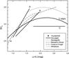 |
Fig. 6 Comparison of various relations for BCK vs. (J − K). Various line styles mark relations from various authors as shown in the figure. The single black point marks the location of the 4000 K, log g = 0, solar metallicity model of Houdashelt et al. (2000). |
For (J − K) < 2 the relations of both Bessell & Wood and Costa & Frogel fall into the cone delineated by our relations A and B (Table 1). Between (J − K) = 1.1 and 2, the two literature relations seem to be the result of a mixture of our two sequences. The bending of the Bessel & Wood relation for higher values of (J − K) may reflect the increasing importance of the relations B and C in that (J − K) range. The maximum difference between our sequences A and B is about 0.5 mag (at (J − K) = 1.5). Since the Bessell & Wood and Costa & Frogel sequences fall in-between these two sequences, their difference from either sequence A or B is between 0.1 and 0.4 mag.
The Montegriffo relation approaches relation A at redder (J − K), and the difference at (J − K) = 1 is approximately 0.1 mag. At this point, the Montegriffo relation and the one of Bessel & Wood are almost identical. However, if a star falls on our sequence B instead of A, the Montegriffo relation may overestimate the bolometric correction by between 0.2 and 0.4 mag.
It is also interesting to have a closer look at the data point given by Houdashelt et al. (2000), which lies very close the crossing point between our sequences A and B. Therefore we propose that from this point on (i.e. for a 4000 K red giant) the bolometric correction relation begins to diverge for stars in the solar neighbourhood. The various literature relations (Bessell & Wood 1984; Costa & Frogel 1996; Montegriffo et al. 1998) also appear to merge into a single relation at (J − K) values bluer than this point.
A yet completely new group are the very red O-rich objects in our sample, which have an almost flat BCK-relation (relation C in Table 1). They cannot be described by any of the relations in the literature. While the number of stars in our sample with (J − K) > 2.0 is comparably small, it is very clear that none of them fall onto an extension of sequence B, but instead form a separate BCK-relation. The general flattening of the Bessell & Wood relation for redder values of (J − K) limits the difference in bolometric correction to a maximum value of 0.4 mag, i.e. BCK would be overestimated by the Bessell & Wood relation by this value.
The Whitelock relation for C-stars seems to provide an average extension of the above-mentioned cone between A and B, which later bends again towards smaller bolometric correction values. This trend is also seen in our relation for the C-rich stars (compare Fig. 1). However, directly comparing our relation for C-rich stars with the Whitelock relation in the same (J − K) range indicates a difference of up to 0.4 mag in BCK. The Whitelock relation generally gives much weaker mbol values than our measurements of C-rich stars.
We note that the Costa & Frogel relation only partly agrees with our results. Why there is far poorer agreement among the BCK relations for C-stars than O-rich stars is not immediately obvious. To determine mbol, Whitelock et al. (2006) performed a spline fit to the photometry from 1.2 to 25 μm, while we use black-body fits to a larger baseline in wavelength, which allows us to consider the possibility of fits with one or two black-bodies. We also did some tests by integrating the flux below a spline fit (as done by Whitelock et al. 2006) and indeed found some small but not systematic differences between the two methods.
4. Conclusions
We have attempted to derive an accurate bolometric correction for AGB stars using a large database of near-infrared photometry and black-body fits performed earlier by one of us (FK). To derive an accurate bolometric correction for e.g. the K-band magnitude for stars of spectral type M, we have found that it is necessary to have L′ filter measurements in addition to the JHK photometry. No clear solution could be found using only the second set of three filters. For the C-type stars, we have established a revised BCK vs. (J − K) relation, which only partly agrees with the findings published in the literature. Understanding these differences will require further study. Summarizing the comparison of our new relations with published BCK vs. (J − K) relations, we have found a maximum difference for BCK of 0.5 mag (plus some additional scatter due to stellar variability) for AGB stars depending on the relation used.
An extension of large infrared surveys such as 2MASS by measurements in the L or L′ band would thus be very valuable to increase our knowledge of AGB stars by enabling us to derive reliable mbol values for them. In a future study, we plan alternatively to look for possible relations for this purpose
using the IRAS [12] mag to compensate for the lack of L-band measurements.
A relation based on our complete data set (all chemistries) was used already in Uttenthaler et al. (2007) to calculate bolometric luminosities for stars in the Galactic bulge.
Acknowledgments
The authors thank the anonymous referee for providing constructive comments on the manuscript leading to significant improvements. F.K. acknowledges funding by the Austrian Science Fund FWF under project number P18939-N16. T.L. acknowledges funding by the FWF under project number P20046-N16.
References
- Aringer, B., Girardi, L., Nowotny, W., Marigo, P., & Lederer, M. T. 2009, A&A, 503, 913 [NASA ADS] [CrossRef] [EDP Sciences] [Google Scholar]
- Bessell, M. S., & Wood, P. R. 1984, PASP, 96, 247 [NASA ADS] [CrossRef] [Google Scholar]
- Bessell, M. S., & Brett, J. M. 1988, PASP, 110, 1134 [NASA ADS] [CrossRef] [Google Scholar]
- Bessell, M. S., Castelli, F., & Plez, B. 1998, A&A, 333, 231 [NASA ADS] [Google Scholar]
- Bouchet, P., Manfroid, J., & Schmider, F. X. 1991, A&AS, 91, 409 [Google Scholar]
- Costa, E., & Frogel, J. A. 1996, AJ, 112, 2607 [NASA ADS] [CrossRef] [Google Scholar]
- Carpenter, J. M. 2001, AJ, 121, 2851 [NASA ADS] [CrossRef] [Google Scholar]
- Frogel, J. A., Persson, S. E., & Cohen, J. G. 1980, ApJ, 239, 495 [NASA ADS] [CrossRef] [Google Scholar]
- Guandalini, R., & Busso, M. 2008, A&A, 488, 675 [NASA ADS] [CrossRef] [EDP Sciences] [Google Scholar]
- Houdashelt, M. L., Bell, R. A., & Sweigart, A. V. 2000, AJ, 119, 1448 [Google Scholar]
- Joint IRAS Science Working Group 1988, IRAS Catalogue and Atlases, Vol. 2 − 6, ed. C. A. Beichmann, G. Neugebauer, H. J. Habing, P. E. Clegg, & T. J. Chester, NASA RP-1190 [Google Scholar]
- Kerschbaum, F. 1995, A&AS, 113, 441 [Google Scholar]
- Kerschbaum, F. 1999, A&A, 351, 627 [NASA ADS] [Google Scholar]
- Kerschbaum, F., & Hron, J. 1994, A&AS, 106, 397 [NASA ADS] [Google Scholar]
- Kerschbaum, F., & Hron, J. 1996, A&A, 308, 489 [NASA ADS] [Google Scholar]
- Kholopov, P. N., Samus, N. N., Frolov, M. S., et al. 1985 − 88, General Catalogue of Variable Stars, 4th edition (Moscow: Nauka Publishing House) [Google Scholar]
- Montegriffo, P., Ferraro, F. R., Origlia, L., & Fusi Pecci, F. 1998, MNRAS, 297, 872 [NASA ADS] [CrossRef] [Google Scholar]
- Uttenthaler, S., Hron, J., Lebzelter, T., et al. 2007, A&A, 463, 251 [NASA ADS] [CrossRef] [EDP Sciences] [Google Scholar]
- Whitelock, P. A., Feast, M. W., Marang, F., & Groenewegen, M. A. T. 2006, MNRAS, 369, 751 [NASA ADS] [CrossRef] [EDP Sciences] [Google Scholar]
Appendix A: Cross-correlation of AGB variables in the GCVS with 2MASS
As a side project, we extended our NIR-database by cross-correlating the long-period variables in the GCVS with the 2MASS catalogue. For that, we first linked the observations from the IRAS Point Source Catalogue to the GCVS data. The coordinates from the point source catalogue were then transformed from epoch 1950.0 to 2000.0 (the epoch of 2MASS). We searched for 2MASS counterparts within a search radius of 15 arcsec around the IRAS point source. In the case of multiple matches, the first selection criterion was the distance to the IRAS coordinate. If two objects were found at similar distance, the colours were taken into account. If no clear decision was possible, the object was rejected from our database. Out of the 6108 IRAS point sources analysed, 5726 stars or 93.7% could be matched unambiguously with a 2MASS source.
In our previous database described in Sect. 2, all photometric data were either obtained in or transformed to the ESO system. To establish all near-infrared data on the same photometric system, we checked the transformation from the 2MASS to the ESO system provided by Carpenter (2001). This check seemed advisable as the Carpenter sample was dominated by comparison stars with (J − K) < 0.5, and the reddest star in his comparison has J − K = 0.9, while the stars in our database have (J − K) values that extend to 1.4. We find that the mean value of the difference is close to zero and there appears to be no significant dependence on colour. The observed scatter around the relation is most likely due to stellar variability.
All Tables
Linear equations for deriving BC from (J − K) using the location of the star in the two-colour plane.
All Figures
|
Fig. 1 Bolometric correction derived from black-body fits vs. (J − K). The upper panel shows the results for O-rich stars (spectral type M or K), while the lower panel presents the reuslts for the C-type stars (filled circles). S-type stars are also shown in the lower panel and are marked with crosses. See text for details. |
| In the text | |
|
Fig. 2 The colour index J − K vs. the bolometric correction for the O-rich stars of our sample that required two black-bodies when fitting their SED. The sample is separated into three groups according to the luminosity ratio of the two black-bodies: L-ratio < 0.013 (filled circles), 0.013 ≤ L-ratio < 0.025 (open circles), and L-ratio ≤ 0.025 (crosses). |
| In the text | |
|
Fig. 3 The colour index (J − K) versus the bolometric correction for the O-rich stars of our sample separated according to their variability type: irregular variables (filled circles), semiregular variables (open circles), and miras (crosses). |
| In the text | |
|
Fig. 4 Two-colour diagram (J − K) vs. (K − L′) for our sample stars, divided into three regions related to three different colour-mbol relations. See Fig. 5. The open circles give the intrinsic colours for giants of spectral type K0, K3, M1, and M5 from Bessell & Brett (1988), respectively. The large filled boxes mark the colours of black-body SEDs from 3500 to 1500 K. |
| In the text | |
|
Fig. 5 The colour index (J − K) versus the bolometric correction for the O-rich stars of our sample separated according to their location in the (J − K) vs. (K − L′) two-colour diagram (see Fig. 4). |
| In the text | |
|
Fig. 6 Comparison of various relations for BCK vs. (J − K). Various line styles mark relations from various authors as shown in the figure. The single black point marks the location of the 4000 K, log g = 0, solar metallicity model of Houdashelt et al. (2000). |
| In the text | |
Current usage metrics show cumulative count of Article Views (full-text article views including HTML views, PDF and ePub downloads, according to the available data) and Abstracts Views on Vision4Press platform.
Data correspond to usage on the plateform after 2015. The current usage metrics is available 48-96 hours after online publication and is updated daily on week days.
Initial download of the metrics may take a while.