| Issue |
A&A
Volume 523, November-December 2010
|
|
|---|---|---|
| Article Number | A87 | |
| Number of page(s) | 9 | |
| Section | Celestial mechanics and astrometry | |
| DOI | https://doi.org/10.1051/0004-6361/201015296 | |
| Published online | 18 November 2010 | |
A precise modeling of Phoebe’s rotation
1
Observatoire de Paris, Systèmes de Référence Temps Espace (SYRTE),
CNRS/UMR8630, Paris,
France
e-mail: This email address is being protected from spambots. You need JavaScript enabled to view it.
;This email address is being protected from spambots. You need JavaScript enabled to view it.
2
Main (Pulkovo) Astronomical Observatory of the Russian Academy of
Sciences, Saint-Petersburg, Russia
e-mail: This email address is being protected from spambots. You need JavaScript enabled to view it.
Received:
29
June
2010
Accepted:
13
August
2010
Abstract
Aims. Although the rotation of some Saturn’s satellites in spin-orbit has already been studied by several authors, this is not the case for the rotation of Phoebe, which stands out because it is non-resonant. The purpose of the paper is to determine for the first time and with precision its precession-nutation motion.
Methods. We adopt an Hamiltonian formalism of the rotation motion of rigid celestial bodies set up by Kinoshita (1977, Celest. Mech., 15, 277) based on Andoyer variables and canonical equations. First we calculate Phoebe’s obliquity at J2000,0 from available astronomical data as well as the gravitational perturbation caused by Saturn on Phoebe’s rotational motion. Then we carry out a numerical integration and compare our results for the precession rate and the nutation coefficients with a purely analytical model.
Results. Our results for Phoebe’s obliquity (23°95) and Phoebe’s precession rate (5580 65/cy) are very close to the respective values for the Earth. Moreover the amplitudes of the nutations (26′′ peak to peak for the nutaton in longitude and 8′′ for the nutation in obliquity) are on the same order as the respective amplitudes for the Earth. We give complete tables of nutation, obtained from a fast fourier transform (FFT) analysis starting from the numerical signals. We show that a purely analytical model of the nutation is not accurate because Phoebe’s orbital elements e, M and LS do not show a simple linear behaviour at all.
Conclusions. The precession and nutation of Phoebe have been calculated for the first time in this paper. We will continue this study in the future by studying the additional gravitational effects of the Sun, of the large satellites such as Titan, as well as Saturn’s dynamical ellipticity.
Key words: planets and satellites: dynamical evolution and stability / celestial mechanics / planets and satellites: individual: Phoebe
© ESO, 2010
1. Introduction
Understanding the rotation of gravitationally interacting bodies with an ever increasing accuracy is an important challenge of celestial mechanics. Many authors have modeled with very high accuracy the rotation of the Earth for instance Woolard (1953), Kinoshita (1977). The other planets of the Solar system followed logically (see for instance Yoder 1997; Rambaux 2007). Today, thanks to new and very precise observational astrometric techniques, the dynamical study of celestial bodies extends to comets, asteroids and satellites (Meyer 2008; Sinclair 1977; Wisdom 1984, 1987).
Yet only a few studies have been made of the rotational motion of Phoebe, the ninth satellite of Saturn, since its discovery in 1899 by Pickering. In 1905, Ross etablished that its motion is retrograde and gave for the first time the orbital elements for the mean equinox and ecliptic of date. Jacobson (1998) determined new orbital elements thanks to Earth-based astrometric observations from 1904 to 1996. More recently Emelyanov(2007) made ephemerides of Phoebe from 1904 to 2027. Others studies have been made of the composition and the inertial parameters of Phoebe (Aleshkina et al. 2010). Phoebe is the only non-synchronous satellite of Saturn with rather well known physical parameters, such as the moments of inertia. Because Phoebe is a dissymetric body (large dynamical flattening and large triaxiality), it is interesting to study its rotation.
We propose here for the first time, to determine the combined motion of precession and nutation of Phoebe considered as a rigid body. After presenting the model (Sect. 2), we describe the orbital motion of Phoebe by fitting the curves of the temporal variations of the orbital elements a,e,M and Ls with polynomial functions. Thanks to a fast fourier transform (FFT), the large periodic variations around the mean elements are analyzed and show that the orbital motion of Phoebe is far from being Keplerian (Sect. 3). Then we determine the motion of precession and nutation of Phoebe by numerical integration using the value of the obliquity obtained in Sect. 4. Finally, after quantifying the validity of the developments done by Kinoshita (1977) for the Earth when applied to Phoebe, an analytical model is constructed.
All our results are compared to the results obtained by Kinoshita for the Earth. We show in Sect. 6 that the analytical model which is very accurate for the Earth is less acurate for Phoebe than the numerical approach to determine the precession and the nutation of Phoebe. This is due to the large periodic departure from the Keplerian motion of the Phoebe’s orbit. We note however that it gives a fairly good approximation for the precession, which is sensitive to the average value.
2. Theoretical equation of the precession-nutation motion
The present study of the rotation of Phoebe considered as a rigid body is based on the
theoritical framework by Kinoshita (1977), who
adopted an Hamiltonian formulation using Andoyer variables (1923) to evaluate the motion of the precession-nutation of the rigid Earth. Here a
simplified model is described and only the variables and the equations used in this paper
are detailed. The rotation of a rigid Phoebe involves three axes: the figure axis, which
coincides with the axis of the largest moment of inertia, the angular momentum axis directed
along  , with G the
amplitude of the angular momentum and a reference axis arbitrarly chosen as the axis
perpendicular to the orbit of Phoebe at a given epoch t (see Fig. 1). The precession and nutation motions are the linear and
the quasi-periodic parts of the motion of the figure axis or of the angular momentum axis
with respect to the reference axis. Assuming that the angle J between the
angular momentum axis and the figure axis is small, as it is for the Earth (for which its
value is less than 1′′), only the motion of the angular momentum axis is
considered here. The motion of this axis with respect to the reference axis is described by
the angles h,I (Andoyer 1923), where
I is the obliquity angle and h is characterizing the
precession-nutation in longitude, which corresponds to the angle between the reference point
γt and the node Q. The
reference point γt is the intersection between
the orbit and the equator of Phoebe at the epoch t , the so-called “departure point”
(Capitaine 1986), and Q is the
ascending node between the plane normal to the angular momentum and the orbital plan. The
Andoyer variables g,l in Fig. 1 are
the angle between the node Q and the node P and the angle
between a meridian origin and the node P, where P is
itself the ascending node between the plane normal to the angular momentum axis and the
equatorial plane. The proper rotation of Phoebe is described by the angle
l + g = Φ. The Hamiltonian related to the rotational
motion of Phoebe is
, with G the
amplitude of the angular momentum and a reference axis arbitrarly chosen as the axis
perpendicular to the orbit of Phoebe at a given epoch t (see Fig. 1). The precession and nutation motions are the linear and
the quasi-periodic parts of the motion of the figure axis or of the angular momentum axis
with respect to the reference axis. Assuming that the angle J between the
angular momentum axis and the figure axis is small, as it is for the Earth (for which its
value is less than 1′′), only the motion of the angular momentum axis is
considered here. The motion of this axis with respect to the reference axis is described by
the angles h,I (Andoyer 1923), where
I is the obliquity angle and h is characterizing the
precession-nutation in longitude, which corresponds to the angle between the reference point
γt and the node Q. The
reference point γt is the intersection between
the orbit and the equator of Phoebe at the epoch t , the so-called “departure point”
(Capitaine 1986), and Q is the
ascending node between the plane normal to the angular momentum and the orbital plan. The
Andoyer variables g,l in Fig. 1 are
the angle between the node Q and the node P and the angle
between a meridian origin and the node P, where P is
itself the ascending node between the plane normal to the angular momentum axis and the
equatorial plane. The proper rotation of Phoebe is described by the angle
l + g = Φ. The Hamiltonian related to the rotational
motion of Phoebe is  (1)Fo
is the Hamiltonian for the free rotational motion defined by
(1)Fo
is the Hamiltonian for the free rotational motion defined by  (2)where
L is the component of the angular momentum axis along the figure axis and
A,B,C are the principal moments of inertia of Phoebe.
E + E′ is a component related to the motion
of the orbit of Phoebe, which is caused by planetary perturbations and has been discussed in
detail in Cottereau & Souchay (2009) when
studying the rotation of Venus. U is the disturbing potential of Saturn,
considered as a point mass and its disturbing potential is given by
(2)where
L is the component of the angular momentum axis along the figure axis and
A,B,C are the principal moments of inertia of Phoebe.
E + E′ is a component related to the motion
of the orbit of Phoebe, which is caused by planetary perturbations and has been discussed in
detail in Cottereau & Souchay (2009) when
studying the rotation of Venus. U is the disturbing potential of Saturn,
considered as a point mass and its disturbing potential is given by
![Mathematical equation: \begin{eqnarray} \label{eq1} U_{1} &=& \frac{\mathtt{\textbf{G}} M'}{r^3} \left[\left[\frac{2C-A-B}{2}\right]P_{2}(\sin \delta )\right.\nonumber\\ &\quad+&\left.\left[\frac{A-B}{4}\right]P_2^{2} (\sin \delta) \cos 2\alpha\right] \end{eqnarray}](/articles/aa/full_html/2010/15/aa15296-10/aa15296-10-eq28.png) (3)
(3)![Mathematical equation: \begin{eqnarray} U_{2}&=&\sum_{n=3}^\infty \frac{\mathtt{\textbf{G}} M'M_{P}a^n}{r^{n+1}}[J_{n}P_{n}(\sin \delta) \nonumber\\ &\quad - &\sum_{m=1}^n{P_{n}^m (\sin\delta) \cdot (C_{nm}\cos m\alpha +S_{nm} \sin m\alpha) }], \end{eqnarray}](/articles/aa/full_html/2010/15/aa15296-10/aa15296-10-eq29.png) (4)
(4)
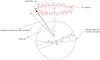 |
Fig. 1 Precession nutation motion. |
 are the classical Legendre
functions given by:
are the classical Legendre
functions given by:  (5)Note that the perturbations
caused by, the other planets, satellites and the Sun, which are a priori of second order,
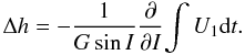
will not be studied in this paper. The variation of the obliquity and the precession angle
is given by
(5)Note that the perturbations
caused by, the other planets, satellites and the Sun, which are a priori of second order,
will not be studied in this paper. The variation of the obliquity and the precession angle
is given by ![Mathematical equation: \begin{eqnarray} \frac{{\rm d}I}{{\rm d}t}&=& \frac{1}{G}\left[\frac{1}{\sin I} \frac{\partial K}{\partial h} - \cot I \frac{\partial K}{\partial g}\right] \nonumber\\ \frac{{\rm d}h}{{\rm d}t}&=& - \frac{1}{G\sin I} \frac{\partial K}{\partial I}\cdot \end{eqnarray}](/articles/aa/full_html/2010/15/aa15296-10/aa15296-10-eq37.png) (6)To
solve these equations, Kinoshita (1977) used Hori’s
method. Because the order of the disturbing function is given by
(6)To
solve these equations, Kinoshita (1977) used Hori’s
method. Because the order of the disturbing function is given by
 (7)the
same method can be applied to Phoebe. Neglecting the very small contribution as the
component E + E′ and applying the first order
of Hori’s method, this yields
(7)the
same method can be applied to Phoebe. Neglecting the very small contribution as the
component E + E′ and applying the first order
of Hori’s method, this yields ![Mathematical equation: \begin{eqnarray} \label{eq2} \Delta I = \frac{1}{G}\left[\frac{1}{\sin I} \frac{\partial}{\partial h} \int U_{1}{\rm d}t-\cot I \frac{\partial}{\partial g} \int U_{1} {\rm d}t\right] \end{eqnarray}](/articles/aa/full_html/2010/15/aa15296-10/aa15296-10-eq39.png) (8)
(8) (9)U1
given by (3) can be expressed as a function
of the longitude λ and the latitude β of Saturn with
respect to the orbit of Phoebe at the epoch t with the transformations described by
Kinoshita (1977) and based on the Jacobi polynomials:
(9)U1
given by (3) can be expressed as a function
of the longitude λ and the latitude β of Saturn with
respect to the orbit of Phoebe at the epoch t with the transformations described by
Kinoshita (1977) and based on the Jacobi polynomials:
![Mathematical equation: \begin{eqnarray} \label{eq4} U_{1}\nonumber & = & \frac{\mathtt{\textbf{G}} M'}{r^3} \Bigg[\frac{2C-A-B}{2}\Bigg(-\frac{1}{4}(3\cos ^2 I-1)\nonumber\\ &\quad - & \frac{3}{4}\sin^2 I \cos 2 (\lambda-h)\Bigg)\nonumber \\ &\quad + & \frac{A-B}{4}\bigg[ \frac{3}{2} \sin^2I \cos(2l+2g)\nonumber \\ &\quad+ & \sum_{\epsilon = \pm 1}\frac{3}{4}(1 + \epsilon \cos I)^2 \cdot \cos 2(\lambda-h-\epsilon l - \epsilon g)\bigg]\Bigg]. \end{eqnarray}](/articles/aa/full_html/2010/15/aa15296-10/aa15296-10-eq44.png) (10)Finally
the motions of precession-nutation in longitude and in obliquity are given starting from
Eqs. (8)–(10) by
(10)Finally
the motions of precession-nutation in longitude and in obliquity are given starting from
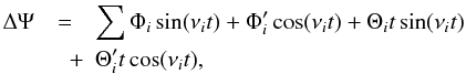
Eqs. (8)–(10) by 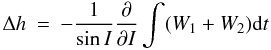 (11)
(11)![Mathematical equation: \begin{eqnarray} \label{eq6} \Delta I &=&\Bigg[\frac{1}{\sin I} \frac{\partial}{\partial h} \int (W_{1}+W_{2}) {\rm d}t \nonumber \\ &\quad -& \cot I \frac{\partial}{\partial g} \int W_{2} dt \Bigg], \end{eqnarray}](/articles/aa/full_html/2010/15/aa15296-10/aa15296-10-eq46.png) (12)where
(12)where
![Mathematical equation: \begin{eqnarray} \label{eq7} W_{1}&=&\frac{\mathtt{\textbf{G}}M'}{Gr^3}\Bigg(\frac{2C-A-B}{2}\Big[-\frac{1}{4}(3\cos ^2 I-1)\nonumber\\ & \quad -& \frac{3}{4}\sin^2 I \cos 2 (\lambda-h)\Big]\Bigg) \\ \label{eq8} W_{2}&=&\frac{\mathtt{\textbf{G}}M'}{Gr^3}\Bigg(\frac{A-B}{4}\Bigg[\frac{3}{2} \sin^2I \cos(2l+2g)\nonumber \\ &\quad +&\sum_{\epsilon=\pm 1}\frac{3}{4}(1+\epsilon \cos I)^2 \nonumber \\&& \cos 2(\lambda-h-\epsilon l-\epsilon g)\Bigg]\Bigg). \end{eqnarray}](/articles/aa/full_html/2010/15/aa15296-10/aa15296-10-eq47.png) Because
W1 does not depend on g, this variable does
not appear in the second part of the right hand side of Eq. (12). Supposing that the components ω1 and
ω2 of Phoebe’s rotation are negligible with respect to the
component ω3 along the figure axis, as it is the case for the
Earth, this yields
Because
W1 does not depend on g, this variable does
not appear in the second part of the right hand side of Eq. (12). Supposing that the components ω1 and
ω2 of Phoebe’s rotation are negligible with respect to the
component ω3 along the figure axis, as it is the case for the
Earth, this yields ![Mathematical equation: \begin{eqnarray} \label{eq9} W_{1} & = & \frac{3\mathtt{\textbf{G}}M'}{\omega r^3} \left(\frac{2C-A-B}{2C}\left[-\frac{1}{12}(3\cos ^2 I-1)\right. \right.\nonumber\\ & \quad -& \left. \left. \frac{1}{4}\sin^2 I \cos 2 (\lambda-h)\right]\right)\\ \label{eq10} W_{2} & = & \frac{3\mathtt{\textbf{G}}M'}{\omega r^3 }\Bigg(\frac{A-B}{4C}\Big[\frac{1}{2} \sin^2I \cos(2l+2g)\nonumber \\ &\quad +& \sum_{\epsilon=\pm 1}\frac{1}{4}(1+\epsilon \cos I)^2 \nonumber \\ && \cos 2(\lambda-h-\epsilon l-\epsilon g)\Big]\Bigg), \end{eqnarray}](/articles/aa/full_html/2010/15/aa15296-10/aa15296-10-eq53.png) where
where
 and
and
 are the
dynamical flattening and the triaxiality of Phoebe. Because the rotation of Phoebe is
retrograde, the conventional notations of the precession and obliquity will be respectively
are the
dynamical flattening and the triaxiality of Phoebe. Because the rotation of Phoebe is
retrograde, the conventional notations of the precession and obliquity will be respectively
 (17)
(17) (18)which are the opposite
of the conventional ones for the Earth (Kinoshita 1977; Souchay et al. 1999).
(18)which are the opposite
of the conventional ones for the Earth (Kinoshita 1977; Souchay et al. 1999).
3. Phoebe’s ephemerides
The ephemerides used in this paper for Phoebe’s orbital motion around Saturn have been constructed by Emelyanov (2007), where the orbital parameters and the coordinates (X,Y,Z) of Phoebe are given in the planeto-equatorial reference frame considered as inertial from the first observation date in 1904 to 2027. The reference point is one of the intersections between Saturn and Earth equatorial planes at J2000.0. To apply the theoretical framework of Kinoshita (1977), the mean elements for the variables a,e,M and Ls are needed. In this section, these elements are calculated in the same way as in Simon et al. (1994) for the planets. The differences betwen the true motion of Phoebe and a Keplerian motion are also studied. Throughout the paper our study is restricted to the time span ranging from 2000.0 to the limit of the ephemeris 2027.0.
3.1. The semi-major axis
The mean element for the semi-major axis for the Earth is a constant (Simon et al. 1994) and the relative variations around this mean
value are on the order 10-5. In comparaison, for Phoebe, approximating
a by a constant does not yield a good accuracy. Figure 2 shows the relative variation of a
around its mean value estimated at  in a 9000 days’ time span. The
variations clearly consist of periodic components with an amplitude on the order of
10-3. The leading oscillations of the signal are determined with a fast
fourier transform (FFT). Table 1 gives the leading
amplitudes and periods of the sinusoids characterizing the signal in Fig. 2, where the central curve represents the residuals after
substraction of these sinusoids.
in a 9000 days’ time span. The
variations clearly consist of periodic components with an amplitude on the order of
10-3. The leading oscillations of the signal are determined with a fast
fourier transform (FFT). Table 1 gives the leading
amplitudes and periods of the sinusoids characterizing the signal in Fig. 2, where the central curve represents the residuals after
substraction of these sinusoids.
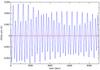 |
Fig. 2 Relative variation of a around the mean value
|
Leading amplitudes and periods characterizing the semi-major axis.
3.2. The mean elements of the orbital parameters
Below the formula for the mean elements of Phoebes′ Keplerian motion
e,M and LS are given,
where M,Ls are the mean
anomaly and mean longitude with respect to the “departure point”
γt. They were obtained by fitting the
curves of the temporal variations of these elements given by Emelyanov (2007) with a polynomial expression at 6th order as was
done for the planets of the solar system (Simon et al. 1994). Considering the limits of the ephemerides, truncating the polynomial
functions at the 6th order looks a sufficient approximation. Thus 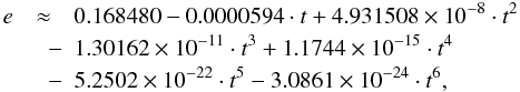 (19)
(19)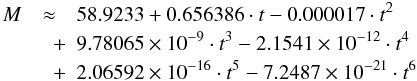 (20)
(20)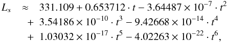 (21)where
t is counted in Julian days, M and
Ls are expressed in degrees. Figure 3 shows the variations of the eccentricity of Phoebe for
a 9000 days’ time span. An important feature of Phoebes’ orbit is the high eccentricity as
well as its very large relative variations (of the order of 10%). As we will see in
Sect. 6, this will be very important in our study
because of the large corresponding variations of
(21)where
t is counted in Julian days, M and
Ls are expressed in degrees. Figure 3 shows the variations of the eccentricity of Phoebe for
a 9000 days’ time span. An important feature of Phoebes’ orbit is the high eccentricity as
well as its very large relative variations (of the order of 10%). As we will see in
Sect. 6, this will be very important in our study
because of the large corresponding variations of  that it causes for the orbit.
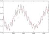 |
Fig. 3 Variation of the eccentricity of Phoebe for a 9000 days’ time span. The central curve represents the polynomial function given by Eq. (19). |
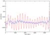 |
Fig. 4 Residuals after substraction of the polynomials given by Eq. (19) from the eccentricity of Phoebe for a 9000 days’ time span. The central curve represents the residuals after substracting the sinusoidal terms of Table 2. |
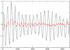 |
Fig. 5 Residuals after substraction of the polynomials given by Eq. (20) from the mean anomaly of Phoebe M for a 9000 days’ time span. The central curve represents the residuals after substracting the sinusoidal terms of Table 2. |
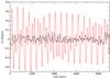 |
Fig. 6 Residuals after substraction of the polynomials given by Eq. (21) from the mean longitude of Phoebe Ls for a 9000 days’ time span. The central curve represents the residuals after substracting the sinusoidal terms of Table 2. |
Figures 4–6 represent the residuals after substraction of the polynomial functions given by Eqs. (19)–(21)from the eccentricity, the mean anomaly and the mean longitude of Phoebe. As already observed for the semi-major axis, the residuals have periodic components, which reach an amplitude of 4° for the mean anomaly.
3.3. Frequencies analysis
Thanks to a fast fourier transform (FFT) analysis the leading ampitudes and the periods of the sinusoids characterizing the signals in Figs. 4–6 are determined and given in Table 2.
Leading amplitudes and periods characterizing the orbital elements e,M, and Ls.
The central curves in Figs. 4–6 represent the residuals after substraction of the leading sinusoidal components of the mean elements. We highlight here that the motion of Phoebe is far from being a quasi-Keplerian motion as is the case for the planets of the solar system. Below the precession-nutation of Phoebe is determined both analytically and numerically. The differences between the results given by the two methods because of the non-Keplerian motion of Phoebe will be significantly increased when compared with the equivalent study for the Earth (Kinoshita 1977). All Phoebe’s parameters involved in the Eqs. (11) and (12), which enable one to calculate the precession and nutation are known except for the obliquity of Phoebe at J2000.0, which represents a fundamental initial condition. It is calculated in the following section.
4. Obliquity of Phoebe at J2000.0
With a similar method as in Cottereau & Souchay (2009), the obliquity is given by  (22)where
Pop and Pp are the unit vectors
directed toward the orbital pole and the pole of rotation of Phoebe at
t0, which are:
(22)where
Pop and Pp are the unit vectors
directed toward the orbital pole and the pole of rotation of Phoebe at
t0, which are:
![Mathematical equation: \begin{eqnarray} \overrightarrow{P_{\rm op}}= \left( \begin{array}{ll} \sin i_{0}& \sin \Omega_{0}\\[2mm] -\sin i_{0}& \cos \Omega_{0} \\[2mm] \cos i_{0} \end{array} \right), \overrightarrow{P_{\rm p}}= \left( \begin{array}{ll} \cos \delta_{\rm p}^{0}& \cos \alpha_{\rm p}^{0} \\[2mm] \sin \alpha_{\rm p}^{0} &\cos \delta_{\rm p}^{0} \\[2mm] \sin \delta_{\rm p}^{0}. \end{array} \right) \end{eqnarray}](/articles/aa/full_html/2010/15/aa15296-10/aa15296-10-eq90.png) (23)i0,
Ω0 are the inclination and the longitude of the ascending node of Phoebe in the
Saturn equatorial reference frame at J2000.0 given by the ephemerides of Emelyanov (2007) and
(23)i0,
Ω0 are the inclination and the longitude of the ascending node of Phoebe in the
Saturn equatorial reference frame at J2000.0 given by the ephemerides of Emelyanov (2007) and  ,
,  are the geo-equatorial coordinates
of the north pole of Phoebe given by Seidelmann et al. (2007). The numerical values of these variables are given in the Appendix. Applying
two rotations to
are the geo-equatorial coordinates
of the north pole of Phoebe given by Seidelmann et al. (2007). The numerical values of these variables are given in the Appendix. Applying
two rotations to  ,
the two unit vectors are expressed in the Saturn equatorial reference frame and the
obliquity at J2000.0 can be determined directly from Eq. (22).
,
the two unit vectors are expressed in the Saturn equatorial reference frame and the
obliquity at J2000.0 can be determined directly from Eq. (22).
ΔΨ = Δh: nutation coefficients in longitude of Phoebe.
Δϵ = ΔI: nutation coefficients in obliquity of Phoebe.
After computation and taking into account the Phoebe retrograd rotation the numerical value
of the obliquity at J2000.0 is  (24)Note that this obliquity
is close to the Earth’s (
(24)Note that this obliquity
is close to the Earth’s ( ). Knowing the obliquity at J2000.0, the
precession-nutation of Phoebe can be determined with the help of Eqs. (11) and (12) in the following sections.
). Knowing the obliquity at J2000.0, the
precession-nutation of Phoebe can be determined with the help of Eqs. (11) and (12) in the following sections.
5. Numerical results of the precession-nutation of Phoebe
With the ephemeris of Emelyanov (2007), the
precession and the nutation in longitude and in obliquity are determined by numerical
integration with an extrapolation-algorithm based on the explicit midpoint rule. We remind
here that the precession and the nutation in longitude and in obliquity are defined as the
variation in space of the angular momentum axis with respect to the reference axis caused by
Saturn’s gravitational perturbation. They correspond to the linear part of
h and the quasi-periodic part of h and
I. Before integration, the planeto-equatorial coordinates
(X,Y,Z) taken from the ephemerides are converted into rectangular
coordinates with respect to the orbital plane, which at their turn are converted into the
spherical coordinates used in Eqs. (11)
and (12). The values of the dynamical
flattening and the triaxiality of Phoebe are taken from Aleshkina et al. (2010). Figures 7
and 8 show Phoebe’s precession-nutation in longitude
and Phoebe’s nutation alone for a 9000 days’ time span (24.6 y). Figure 9 shows the nutation in obliquity for a 2000 days’ time span (5.47 y).
Note that 9000 days correspond to the limit of the ephemerides. The 2000 days’ time span of
the nutation in obliquity is chosen in order to clearly see the leading oscillations. The
precession and the leading oscillations of the nutation in longitude and in obliquity are
determined by a linear regression and a FFT. Our value obtained for the precession of
Phoebe is  (25)where t
is counted in Julian centuries. Note that this value for the precession in longitude is very
close to the precession for the Earth (
(25)where t
is counted in Julian centuries. Note that this value for the precession in longitude is very
close to the precession for the Earth ( cy). So the effect of the
tidal torque of Saturn on the precession of Phoebe is roughly the same as the combined
gravitational effect of the Moon and Sun on the precession of the Earth. The physical
dissymmetry (high values of the dynamical flattening and of the triaxiality) of Phoebe which
directly increase the amplitude of the precession, are compensated by its slow revolution
and fast rotation (see Eq. (15)) .
cy). So the effect of the
tidal torque of Saturn on the precession of Phoebe is roughly the same as the combined
gravitational effect of the Moon and Sun on the precession of the Earth. The physical
dissymmetry (high values of the dynamical flattening and of the triaxiality) of Phoebe which
directly increase the amplitude of the precession, are compensated by its slow revolution
and fast rotation (see Eq. (15)) .
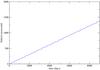 |
Fig. 7 Precession and the nutation of Phoebe in longitude for a 9000 days’ time span. |
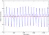 |
Fig. 8 Nutation of Phoebe in longitude for a 9000 days’ time span.The central curve represents the residual after substracting the sinusoidal terms of the Table 3. |
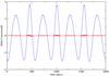 |
Fig. 9 Nutation of Phoebe in obliquity for a 2000 days’ times span.The central curve represents the residual after substracting the sinusoidal terms of the Table 4. |
 (26)where
 and
νi are the leading amplitudes and the
frequencies of the sinusoidal terms and can be found in Table 3. Similarly, the nutation in obliquity is given by
and
νi are the leading amplitudes and the
frequencies of the sinusoidal terms and can be found in Table 3. Similarly, the nutation in obliquity is given by 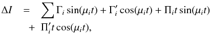 (27)where
 and
μi are given in Table 4. The corresponding arguments for a combination of
Phoebe’s mean longitude and mean anomaly are determined empirically and given when they have
been clearly identified. The residuals after substraction of Eqs. (26) and (27) to the results of the numerical integration are the flat curves in
Figs. 8 and 9.
and
μi are given in Table 4. The corresponding arguments for a combination of
Phoebe’s mean longitude and mean anomaly are determined empirically and given when they have
been clearly identified. The residuals after substraction of Eqs. (26) and (27) to the results of the numerical integration are the flat curves in
Figs. 8 and 9.
The nutation in obliquity is dominated by two frequencies associated with the arguments
2Ls and
2Ls + M with respective
periods 275.13 d and 183.45 d. In addition to these two frequencies, the nutation in
longitude also presents another leading component with argument
2Ls − M. The components
that are not identified in Tables 3 and 4 those with period 497 d and 260 d, are already pointed
out in Tables 1 and 2 (see Sect. 3). They probably come from the
non-Keplerian motion of Phoebe. As for the precession, the nutations in longitude and in
obliquity of Phoebe, which show peak to peak variations of 26′′ or 8′′
are on the same order as the nutation of the Earth (with a factor  and
and  ). Because the value of
the triaxiality ishigh (Aleshkina et al. 2010), it is
interesting to evaluate its effect on Phoebe’s nutation. This effect is determined by
Eqs. (11) and (12) taking only into account the component
depending on in Eqs. (15) and (16). Figures 10 and 11 show the nutation in longitude and in obliquity
depending on the triaxiality for a 10 days’ times span beginning at 410 days. This short
time span is chosen to clearly see the high frequency oscillation to Phoebe’s rotation with
a period roughly half of the proper rotation of Phoebe (9 h) and the higher amplitude of the
whole signal. Thus we remark that despite the large triaxiality of Phoebe, its effect on the
nutation in longitude and in obliquity, at the level of a few 10-3 arcsec
amplitude, is very small. As explained already for the precession, the effect of the
disymmetry of Phoebe, which is characterized by a very high value of its triaxiality, is
compensated by its very fast rotation, which strongly decreases the amplitude of the signal
after integration.
). Because the value of
the triaxiality ishigh (Aleshkina et al. 2010), it is
interesting to evaluate its effect on Phoebe’s nutation. This effect is determined by
Eqs. (11) and (12) taking only into account the component
depending on in Eqs. (15) and (16). Figures 10 and 11 show the nutation in longitude and in obliquity
depending on the triaxiality for a 10 days’ times span beginning at 410 days. This short
time span is chosen to clearly see the high frequency oscillation to Phoebe’s rotation with
a period roughly half of the proper rotation of Phoebe (9 h) and the higher amplitude of the
whole signal. Thus we remark that despite the large triaxiality of Phoebe, its effect on the
nutation in longitude and in obliquity, at the level of a few 10-3 arcsec
amplitude, is very small. As explained already for the precession, the effect of the
disymmetry of Phoebe, which is characterized by a very high value of its triaxiality, is
compensated by its very fast rotation, which strongly decreases the amplitude of the signal
after integration.
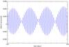 |
Fig. 10 Effect of the triaxiality on the nutation in longitude for a 10 days’ time span. |
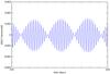 |
Fig. 11 Effect of the triaxiality on the nutation in obliquity for a 10 days’ time span. |
The goal now is to determine an analytical model to describe the precession-nutation of
Phoebe and to compare it with our numerical results. Below the effect of the triaxiality on
the nutation will be ignored and the  in
Eqs. (13) and (14) are replaced by
in
Eqs. (13) and (14) are replaced by  .
.
6. Construction of an analytical model for the precession-nutation of Phoebe
Many authors have made an analytical model of Earth’s rotation in order to understand the causes of the observed motion and to be able to predict it (Kinoshita 1977; Bretagnon et al. 1997; Roosbeek & Dehant 1997; Souchay et al. 1999). In this approach, it is interesting to build an analytical model based on the model of Kinoshita for the Earth to determine the precession and the nutation of Phoebe.
To solve analytically Eqs. (11) and (12), Kinoshita (1977) developed  and
and  as a function of time,
through the variables M and Ls
taking the eccentricity as a small parameter:
as a function of time,
through the variables M and Ls
taking the eccentricity as a small parameter: 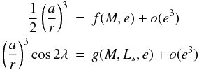 (28)The
detailed demonstration is presented in Kinoshita (1977). Because the eccentricity of the Earth is small, truncating the development
at the 3rd order is a sufficient approximation. But the eccentricity of Phoebe is higher (by
one order) than the eccentricity of the Earth (0.18 instead 0.0167). Moreover, as we have
seen before, Phoebe’s orbital elements are undergoing intensive variations. Then the
relative error made by replacing and by the developments such
as Eq. (28) need to be quantified. To that
purpose, and are developed as for the
Earth, but with the real values of
e,M,LS taken in the
ephemerides of Emelyanov (2007), instead of a linear
value (for e,M ans Ls) for the
Earth.
(28)The
detailed demonstration is presented in Kinoshita (1977). Because the eccentricity of the Earth is small, truncating the development
at the 3rd order is a sufficient approximation. But the eccentricity of Phoebe is higher (by
one order) than the eccentricity of the Earth (0.18 instead 0.0167). Moreover, as we have
seen before, Phoebe’s orbital elements are undergoing intensive variations. Then the
relative error made by replacing and by the developments such
as Eq. (28) need to be quantified. To that
purpose, and are developed as for the
Earth, but with the real values of
e,M,LS taken in the
ephemerides of Emelyanov (2007), instead of a linear
value (for e,M ans Ls) for the
Earth.
6.1. Test for the developments of  and
and 
In this section, the developments of and done by Kinoshita (1977) for the Earth and by Cottereau & Souchay (2009) for Venus
are tested for Phoebe. We used the same methods as in Cottereau & Souchay (2009) to determine the development of
. As the eccentricity of Phoebe is
high, the development at the 3rd order as done by Cottereau & Souchay (2009) for Venus is insufficient because it yields
relative errors on the order of 4 × 10⁻³. This is because of the slow
convergence of the development, which must be carried out up to 6th order in our case, if
we want to reach a relative 10-4 accuracy. Figure 12 shows the discrepancies between the numerical and the
semi-analytical results using this developments both to the 3rd and 6th order. This shows
that high order developments are needed when taking into account highly eccentric orbits
as Phoebe’s one.
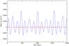 |
Fig. 12
|

For the developments of , the same conclusion is obtained. Figure 13 shows the discrepancies between the numerical and the
semi-analytical results using the developments of  , to 3rd and 6th order. The difference descreases
from 03 to 001 (peak to
peak). The developments are given by
, to 3rd and 6th order. The difference descreases
from 03 to 001 (peak to
peak). The developments are given by 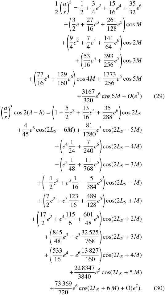
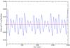 |
Fig. 13
|

6.2. Analytical model of Phoebe
To express and by purely analytical functions, Kinoshita
replaced e,M,LS by their
linear mean values. For Venus, the same method is used in Cottereau & Souchay
(2009), who replaced
e,M,LS by their linear
mean values given by Simon et al. (1994). Using the
mean elements of Sect. (2) and the developments given
by Eqs. (29) and (30), an analytical model is obtained. As
explained in Kinoshita & Souchay (1990) and
Cottereau et al. (2010) for the Earth and for Venus,
the difference between the nutation computed by analytical tables and the numerical
integration is small (on the order of 10-5) and caused by the indirect
planetary effects on the planet. For Phoebe, this difference is also caused by indirect
perturbations, but cannot be ignored as will be shown below. Replacing the semi-major axis
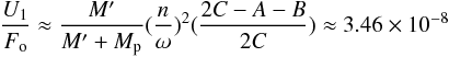
in Eqs. (11) and (12) by  (Sect. 3), Δh and
ΔI depend directly on the scaling factor
KS:
(Sect. 3), Δh and
ΔI depend directly on the scaling factor
KS:
 (31)where
is the
dynamical flattening of Phoebe, ω the angular velocity of Phoebe and
n the mean motion of Phoebe given by
(31)where
is the
dynamical flattening of Phoebe, ω the angular velocity of Phoebe and
n the mean motion of Phoebe given by
 (32)The
numerical value is directly deduced from the values of the A,B,C and
ω taken from Aleshkina et al. (2010) and Bauer et al. (2004). Note that
this scaling factor is very close to Earth’s (110366 by Julian cy). As seen
in Sect. 2 the precession of Phoebe corresponds to
the polynomial part of Eq. (11) and can be
directly determined by
(32)The
numerical value is directly deduced from the values of the A,B,C and
ω taken from Aleshkina et al. (2010) and Bauer et al. (2004). Note that
this scaling factor is very close to Earth’s (110366 by Julian cy). As seen
in Sect. 2 the precession of Phoebe corresponds to
the polynomial part of Eq. (11) and can be
directly determined by 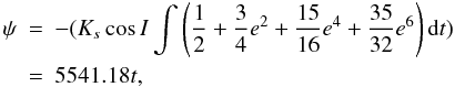 (33)where
e is replaced by the linear part of Eq. (19). The discrepancies between the precession as computed by
analytical integration and that given by Eq. (25) are on the order of 1% and show that the analytical model describes
accuratily the precession of Phoebe. Replacing
e,M,LS in the
developments (29) and (30) by the linear part of Eqs. (19)–(21), the nutation of Phoebe is determined by analytical integration.
Figures 14 and 15 show the differences between the nutation in longitude and in obliquity of
the angular momentum axis from a purely analytical formulation and numerical integration
on 9000 days’ time span. These differences are compared to the residuals obtained in
Sect. 5 after substraction Eqs. (26) and (27) determined by FFT to the numerical signal (central curves in the
Figs. 14 and 15).
(33)where
e is replaced by the linear part of Eq. (19). The discrepancies between the precession as computed by
analytical integration and that given by Eq. (25) are on the order of 1% and show that the analytical model describes
accuratily the precession of Phoebe. Replacing
e,M,LS in the
developments (29) and (30) by the linear part of Eqs. (19)–(21), the nutation of Phoebe is determined by analytical integration.
Figures 14 and 15 show the differences between the nutation in longitude and in obliquity of
the angular momentum axis from a purely analytical formulation and numerical integration
on 9000 days’ time span. These differences are compared to the residuals obtained in
Sect. 5 after substraction Eqs. (26) and (27) determined by FFT to the numerical signal (central curves in the
Figs. 14 and 15).
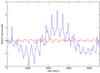 |
Fig. 14 Difference between the nutation in longitude of the analytical and numerical integration for 9000 days’ time span. The flat curve represents the residual after substraction (26) to the nutation signal in longitude obtained by numerical integration. |
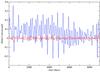 |
Fig. 15 Difference between the nutation in obliquity of the analytical and numerical integration for 9000 days’ time span. The flat curve represents the residual after substraction (27) to the nutation signal in obliquity obtained by numerical integration. |
Figures 14 and 15 show that the semi-analytical functions characterizing the nutation of Phoebe in longitude and in obliquity determined thanks to a FFT are more accurate than those obtained by a pure analytically integration (with linear values of e,M,Ls). The purely analytical model restricts the expressions of the functions that describe the orbital elements. For the Earth (Kinoshita & Souchay 1990) and for Venus (Cottereau et al. 2010), this model is very satisfying because their motions are close to Keplerian and consequently the orbital parameters can be replaced by linear functions. Because the motion of Phoebe is highly disturbedcompared to the planets of the solar system, the curves of the temporal variations of the orbital elements (Emelyanov 2007) cannot be fitted by simple functions as shown by the large variations around the mean elements in Sect. 3. Thus the analytical model does not describe the periodic components due to the indirect effect of the Sun or of the other satellites of Saturn. In contrast these effects are directly taken into account when using the functions given by Eqs. (26) and (27) because the FFT approach followed in Sect. 5 is better suited to describe quasi-periodic motion. However, the precession is less sensitive to these periodic variations, which are averaged during the calculation. This explains the similarity of the precession rate given by the two models. To conclude, the purely analytical model set by Kinoshita (1977) for the Earth gives a good first approximation of the nutation of Phoebe but a more sophisticated analytical model is needed if one wants a precision down to the 10-5 level. We state here that this accuracy is iherent to our model and is independant of the uncertainties in the observations. This shows that we are limited only by the uncertainties on the input data.
7. Conclusion
The purpose of this paper was to calculate for the first time the combined motion of precession and nutation of Saturn’s satellite Phoebe.
One of the important steps in our study was to describe the orbital motion of Phoebe by
fitting the curves of the temporal variations of the orbital elements a,e,M
and Ls with polynomial functions. As shown in
Fig. 2, the periodic variations of the semi-major
axis around its mean value with a relative amplitude of the order on 10-3 are
clearly due to the perturbing effects of other celestial bodies like the Sun. The orbital
motion is far from be a Keplerian one, as shown by the large polynomial expressions of
e,M and Ls, and by the large
sinusoidal amplitudes characterizing the residuals after substraction of these polynomials.
Applying the theoritical framework already used by Kinoshita (1977) for the Earth, the precession and the nutation motion of Phoebe are
determined both analytically and from numerical integration of the equations of motion. We
found that the precession-nutation motion of Phoebe undergoing the gravitational
perturbation of Saturn is quite similar to the Earth undergoing the gravitational effect of
both the Moon and the Sun. Thus our value for the precession of Phoebe, that is to say
558065 cy, is very close to the corresponding
value for the Earth (5081"/cy) and the nutation in longitude and in obliquity of Phoebe with
peak to peak variations of 26′′ and 8′′ are of the same order on
amplitude as the nutation of the Earth (36′′ and 18′′ peak to peak).
Moreover Phoebe’s obliquity ( ) is roughly the same as the Earth’s
(). Note that the physical dissymmetry (high value
of the dynamical flattening and of the triaxiality) and the high eccentricity of Phoebe,
which direclty increases the amplitude of the precession and the nutation, is compensated by
its slow revolution and fast rotation.
) is roughly the same as the Earth’s
(). Note that the physical dissymmetry (high value
of the dynamical flattening and of the triaxiality) and the high eccentricity of Phoebe,
which direclty increases the amplitude of the precession and the nutation, is compensated by
its slow revolution and fast rotation.
In Cottereau & Souchay (2009) we have demonstrated that the effects of the large triaxiality of Venus on its nutation are on the same order of magnitude as the effects of the dynamical flattening. By contrast, the effects of the large triaxiality of Phoebe on its nutation are compensated by its fast rotation and decrease the of amplitude, which becomes negligible compared to the dynamical flattening.
We also investigated the possibility to construct analytical tables of Phoebe nutation, as was done for the Earth. Because Phoebe has a high eccentricity, the analytical developments at the 3th order given by Kinoshita (1977) for the Earth are not valid. We must carry out the developments up to 6th order to reach a relative 10-4 accuracy.
Thus although the amplitude of the nutation motion is close to the Earth’s, we demonstrated that the analytical model used by Kinoshita for the Earth does not describe the nutation motion of a disturbed body like Phoebe with the same accuracy. This analytical model does not take into account the large perturbing effects of the celestial bodies on the orbit of the satellite.
To describe the nutation motion of Phoebe a FFT approach is better than a pure analytical integration done with linear expressions for e,M and LS as shown Figs. 14 and 15. The FFT analysis is better able to describe the periodic variations characterizing the nutation signals of Phoebe. These periodic variations are averaged during the calculation of the precession, which lessens the discrepancies between the two models.
To conclude, we have shown that the analytical model set by Kinoshita (1977) gives a good first approximation of the precession-nutation of Phoebe, but further analytical developments are needed to reach the same accuracy as for the terrestrial planets.
This work can be a starting point for further studies such as the study of another very precise analytical model of the rotation of Phoebe by taking into account effects ignored in this paper, as for instance the direct effects of the Sun, of Titan and of Saturn’s dynamical flattening. Such a model is required to develop the long’s term ephemerides of Phoebe’s rotation, which should require long’s term orbital ephemerides, which are not yet available.
References
- Aleshkina, E. Y., Devyatkin, A. V., & Gorshanov, D. L. 2010, IAU Symp., 263, 141 [NASA ADS] [Google Scholar]
- Andoyer H. 1923, Cours de Mécanique Céleste (Paris: Gauthier-Villars et cie) [Google Scholar]
- Bauer, J. M., Buratti, B. J., Simonelli, D. P., & Owen, W. M., Jr. 2004, ApJ, 610, L57 [NASA ADS] [CrossRef] [Google Scholar]
- Bretagnon P., Rocher P., & Simon J. L. 1997, A&A, 319, 305 [NASA ADS] [Google Scholar]
- Capitaine N., Souchay J., & Guinot B. 1986, Celest. Mech., 39, 283 [NASA ADS] [CrossRef] [Google Scholar]
- Cottereau, L., & Souchay, J. 2009, A&A, 507, 1635 [NASA ADS] [CrossRef] [EDP Sciences] [Google Scholar]
- Cottereau, L., Souchay, J., & Aljbaae, S. 2010, A&A, 515, A9 [NASA ADS] [CrossRef] [EDP Sciences] [Google Scholar]
- Emelyanov, N. V. 2007, A&A, 473, 343 [NASA ADS] [CrossRef] [EDP Sciences] [Google Scholar]
- Jacobson, R. A. 1998, A&AS, 128, 7 [Google Scholar]
- Kinoshita H. 1977, Celest. Mech., 15, 277 [Google Scholar]
- Kinoshita, H., & Souchay, J. 1990, Celest. Mech. Dyn. Astron., 48, 187 [NASA ADS] [CrossRef] [Google Scholar]
- Meyer, J., & Wisdom, J. 2008, Icarus, 193, 213 [NASA ADS] [CrossRef] [Google Scholar]
- Rambaux, N., Lemaitre, A., & D’Hoedt, S. 2007, A&A, 470, 741 [NASA ADS] [CrossRef] [EDP Sciences] [Google Scholar]
- Roosbeek, F., & Dehant, V. 1997, IAU Joint Discussion, 3 [Google Scholar]
- Ross, F. E. 1905, Annals of Harvard College Observatory, 53, 101 [NASA ADS] [Google Scholar]
- Seidelmann, P. K., Archinal, B. A., A’Hearn, M. F., et al. 2007, Celest. Mech. Dyn. Astron., 98, 155 [NASA ADS] [CrossRef] [Google Scholar]
- Simon J. L.,Bretagnon, P., Chapront, J., et al. 1994, A&A, 282, 663 [NASA ADS] [Google Scholar]
- Sinclair, A. T. 1977, MNRAS, 180, 447 [NASA ADS] [Google Scholar]
- Souchay, J., Loysel, B., Kinoshita, H., & Folgueira, M. 1999, A&AS, 135, 111 [Google Scholar]
- Wisdom, J. 1987, AJ, 94, 1350 [NASA ADS] [CrossRef] [Google Scholar]
- Wisdom, J., Peale, S. J., & Mignard, F. 1984, Icarus, 58, 137 [NASA ADS] [CrossRef] [Google Scholar]
- Woolard, E. W. 1953, Astronomical papers prepared for the use of the American ephemeris and nautical almanac (Washington), 15, 1 [Google Scholar]
- Yoder, C. F., & Standish, E. M. 1997, J. Geophys. Res., 102, 4065 [Google Scholar]
Appendix A Appendix A
Numerical values.
All Tables
All Figures
|
Fig. 1 Precession nutation motion. |
| In the text | |
|
Fig. 2 Relative variation of a around the mean value
|
| In the text | |
|
Fig. 3 Variation of the eccentricity of Phoebe for a 9000 days’ time span. The central curve represents the polynomial function given by Eq. (19). |
| In the text | |
|
Fig. 4 Residuals after substraction of the polynomials given by Eq. (19) from the eccentricity of Phoebe for a 9000 days’ time span. The central curve represents the residuals after substracting the sinusoidal terms of Table 2. |
| In the text | |
|
Fig. 5 Residuals after substraction of the polynomials given by Eq. (20) from the mean anomaly of Phoebe M for a 9000 days’ time span. The central curve represents the residuals after substracting the sinusoidal terms of Table 2. |
| In the text | |
|
Fig. 6 Residuals after substraction of the polynomials given by Eq. (21) from the mean longitude of Phoebe Ls for a 9000 days’ time span. The central curve represents the residuals after substracting the sinusoidal terms of Table 2. |
| In the text | |
|
Fig. 7 Precession and the nutation of Phoebe in longitude for a 9000 days’ time span. |
| In the text | |
|
Fig. 8 Nutation of Phoebe in longitude for a 9000 days’ time span.The central curve represents the residual after substracting the sinusoidal terms of the Table 3. |
| In the text | |
|
Fig. 9 Nutation of Phoebe in obliquity for a 2000 days’ times span.The central curve represents the residual after substracting the sinusoidal terms of the Table 4. |
| In the text | |
|
Fig. 10 Effect of the triaxiality on the nutation in longitude for a 10 days’ time span. |
| In the text | |
|
Fig. 11 Effect of the triaxiality on the nutation in obliquity for a 10 days’ time span. |
| In the text | |
|
Fig. 12
|
| In the text | |
|
Fig. 13
|
| In the text | |
|
Fig. 14 Difference between the nutation in longitude of the analytical and numerical integration for 9000 days’ time span. The flat curve represents the residual after substraction (26) to the nutation signal in longitude obtained by numerical integration. |
| In the text | |
|
Fig. 15 Difference between the nutation in obliquity of the analytical and numerical integration for 9000 days’ time span. The flat curve represents the residual after substraction (27) to the nutation signal in obliquity obtained by numerical integration. |
| In the text | |
Current usage metrics show cumulative count of Article Views (full-text article views including HTML views, PDF and ePub downloads, according to the available data) and Abstracts Views on Vision4Press platform.
Data correspond to usage on the plateform after 2015. The current usage metrics is available 48-96 hours after online publication and is updated daily on week days.
Initial download of the metrics may take a while.