| Issue |
A&A
Volume 523, November-December 2010
|
|
|---|---|---|
| Article Number | A4 | |
| Number of page(s) | 16 | |
| Section | Cosmology (including clusters of galaxies) | |
| DOI | https://doi.org/10.1051/0004-6361/201014347 | |
| Published online | 10 November 2010 | |
Reionization by UV or X-ray sources
1
LERMA, Observatoire de Paris,
61 Av. de l’Observatoire,
75014
Paris,
France
2
Scuola Normale Superiore,
Piazza dei Cavalieri 7,
56126
Pisa,
Italy
e-mail: sunghye.baek@sns.it
3
Université Pierre et Marie Curie,
4 place Jussieu, 75005
Paris,
France
4
GEPI, Observatoire de Paris, 5 place Jules Janssen, 92195
Meudon Cedex,
France
5
Laboratoire d’Astrophysique, École Polytechnique Fédérale de
Lausanne (EPFL), Swizerland
Received:
3
March
2010
Accepted:
3
August
2010
We present simulations of the 21-cm signal during the epoch of reionization. We focus on properly modeling the absorption regime in the presence of inhomogeneous Wouthuysen-Field effect and X-ray heating. We ran radiative transfer simulations for three bands in the source spectrum (Lyman, UV, and X-ray) to fully account for these processes. We find that the brightness temperature fluctuation of the 21 cm signal has an amplitude greater than 100 mK during the early reionization, up to 10 times greater than the typical amplitude of a few 10 mK obtained during the later emission phase. More importantly, we find that even a rather high contribution from QSO-like sources only damps the absorption regime without erasing it. Heating the IGM with X-ray takes time. Our results show that observations of the early reionization will probably benefit from a higher signal-to-noise value than during later stages. After analyzing the statistical properties of the signal (power spectrum and PDF) we find three diagnostics to constrain the level of X-ray, hence the nature of the first sources.
Key words: dark ages, reionization, first stars / radiative transfer / HII regions / quasars: general / intergalactic medium / early Universe
© ESO, 2010
1. Introduction
The epoch of reionization (EoR) started with the formation of the first sources of light around z = 15−30. As shown by the Gunn-Peterson effect (Gunn & Peterson 1965) in the spectra of high-redshift quasars (QSO) (e.g., Fan et al. 2006), the universe was fully reionized by z ~ 6. WMAP 5-year results show that the optical depth for the Thomson scattering of CMB photons traveling through the reionizing universe is τ = 0.084 ± 0.016 (Komatsu et al. 2009). Together with the Gunn-Peterson data, this strongly favors an extended reionization period between z > 11 and z = 6.
While other observations, such as the Lyman-α emitter luminosity function (Ouchi et al. 2009), may produce other constraints on the history of reionization in the next few years, the most promising is the observation of the 21-cm line in the neutral IGM using large radio-interferometers (LOFAR1, MWA2, GMRT3, 21-CMA4, SKA5). The signal will be observed in emission or in absorption against the CMB continuum. Both theoretical modeling (Madau et al. 1997; Furlanetto et al. 2006) and simulations (e.g., Ciardi & Madau 2003; Gnedin 2004; Mellema et al. 2006b; Lidz et al. 2008; Ichikawa et al. 2010; Thomas et al. 2009) show that the brightness temperature fluctuations of the 21 cm signal have an amplitude of a few 10 mK in emission, on scales from tens of arcmin down to sub-arcmin. With this amplitude, and ignoring the issue of foreground cleaning residuals, statistical quantities such as the three-dimensional power spectrum should be measurable with LOFAR or MWA with a few 100 h integration (Morales & Hewitt 2004; Furlanetto et al. 2006; Lidz et al. 2008). In absorption however, the amplitude of the fluctuations may exceed 100 mK (Gnedin 2004; Santos et al. 2008; Baek et al. 2009), the exact level depending on the relative contribution of the X-ray and UV sources to the process of cosmic reionization.
The signal will be seen in absorption during the initial phase of reionization, probably at z > 10, when the accumulated amount of emitted X-ray is not yet sufficient to raise the IGM temperature above the CMB temperature. The duration and intensity of this absorption phase, regulated by the spectral energy distribution (SED) of the sources, are crucial. SKA precursors able to probe the relevant frequency range, 70–140 MHz, may benefit from a much higher signal-to-noise than during later periods in the EoR. However, if the absorption phase is confined at redshifts above 15, RFI and the ionosphere will become an problem. Quite clearly, the different types of sources of reionization and different formation histories produce very different properties for the 21-cm signal. It is therefore important for future observations to explore the range of astrophysically plausible scenarios using numerical simulations.
To properly model the signal, it is necessary to use >100 h-1Mpc box sizes (Barkana & Loeb 2004). Together with a large box size, it is desirable to resolve halos with masses down to 108 M⊙ as these contain sources (able to cool below their virial temperature by atomic processes), or even minihalos with masses down to 104 M⊙ became they act as an efficient photon sink because of their high recombination rate (Iliev et al. 2005). As this work focuses on improving the physical modeling, we restrict ourselves to resolving halos with a mass 1010 M⊙ or higher. Indeed, simulating the absorption phase correctly, as we do in this work, requires a more extensive and more costly implementation of radiative transfer. We are exploring the direct implication of this improved physical modeling, and will turn to better mass resolution in the near future.
There are three bands in the sources SED that influence the level of the 21 cm signal: the Lyman band, the ionizing UV band, and the soft X-ray band. Lyman band photons are necessary to decouple the spin temperature of hydrogen from the CMB temperature through the Wouthuysen-Field effect (Wouthuysen 1952; Field 1958), and make the EoR signal visible. UV band photons are of course responsible for the ionization of the IGM, and soft X-rays are able to preheat the neutral gas ahead of the ionizing front, deciding whether the decoupled spin temperature is less (weak preheating) or greater (strong preheating) than the CMB temperature. While a proper modeling should perform the full 3D radiative transfer in all 3 bands, a simpler modeling has often been used in previous works. Indeed, for the usual source SEDs and source formation histories, once the average ionization fraction of the universe is greater than ~10%, the background flux of Lyman-α photons is so high that the hydrogen spin temperature is fully coupled to the kinetic temperature by the Wouthuysen-Field effect (Baek et al. 2009). Thereafter, computing the Lyman band radiative transfer is unnecessary. In the same spirit, it has usually been assumed that the preheating of the IGM by soft X-ray was strong enough to raise the kinetic temperature much higher than the CMB temperature everywhere early in the EoR. However, both assumptions fail during the early reionization: the absorption phase. Even in the later part of reionization the second assumption may fail, depending on the nature of the sources. We will quantify this possibility in this paper. Computing the full radiative transfer in all three bands is necessary to study the absorption regime. Indeed, fluctuations in the local Lyman-α flux induce fluctuations in the spin temperature (while the Wouthuysen-Field effect is not yet saturated), which, in turn, modify the power spectrum of the 21 cm signal (Barkana & Loeb 2005; Semelin et al. 2007; Chuzhoy & Zheng 2007; Naoz & Barkana 2008; Baek et al. 2009). The same is true for the fluctuations in the local flux of X-ray photons (Pritchard & Furlanetto 2007; Santos et al. 2008).
Let us emphasize however that, in modeling Lyman-α and X-ray fluctuations, Barkana & Loeb (2005), Naoz & Barkana (2008), Pritchard & Furlanetto (2007) and Santos et al. (2008) all use the semi-analytical approximation that the IGM has a uniform density of absorbers and ignore wing effects in the radiative transfer of Lyman-α photons. Semelin et al. (2007) and Chuzhoy & Zheng (2007) have shown that these wing effects do exist. Moreover, once reionization is under way, ionized bubbles create sharp fluctuations in the number density of absorbers (not to mention simple matter density fluctuations). In this work, for the first time, we present results based on simulations with full radiative transfer for both Lyman-α and X-ray photons.
What are the possible candidates as sources of reionization? Usually, two categories are considered: ionizing UV sources (Pop II and III stars), and X-ray sources (quasars). When we study 21 cm absorption, however, we must distinguish between Pop II and Pop III stars beyond the large difference in luminosity per unit mass of formed star. Indeed Pop II stars have a three times larger Lyman band to ionizing UV band luminosity ratio than Pop III stars. It means that the 21 cm signal will reach its full power (near saturated Wouthuysen-Field effect) at a lower average ionization fraction for Pop II stars than for Pop III stars. The relevant question is: how long do Pop III stars dominate the source population before Pop II stars take over? The answer to this question, related to the whole process of star formation, feedback and metal enrichment of the IGM, is a difficult one. At this stage, state of the art numerical simulations of the EoR use simple prescriptions in the best case (e.g. Iliev et al. 2007), or simply ignore this issue.
The other category of sources are X-ray sources. They may be mini-quasars, X-ray binaries, supernovae (Oh 2001; Glover & Brand 2003), or even more exotic candidates such as dark stars (Schleicher et al. 2009). The exact level of emission from these sources is a matter of speculation. The generally accepted view is that stars dominate over X-ray sources and are sufficient to drive reionization (Shapiro & Giroux 1987; Giroux & Shapiro 1996; Madau et al. 1999; Ciardi et al. 2003). Recently, Volonteri & Gnedin (2009) supported the opposite view. While, in their models, X-ray sources are marginally able to complete reionization by z ~ 6, they find a very low contribution from stars. Indeed they rely on Gnedin et al. (2008) who find, using numerical simulations, a negligible escape fraction for ionizing radiations from galaxies with total mass less than a few 1010 M⊙, who should actually contribute to 90% of the ionizing photon production during the EoR (Choudhury & Ferrara 2007). While the physical modeling in their innovative simulations is quite detailed, this surprizing behavior of the escape fraction definitely needs to be checked at higher resolution and with different codes. For the time being the best simulations can only explore a plausible range of X-ray contributions, and quantify the impact on observables. When the observations become available we would like to be able, using simulation results, to derive tight constraints on the relative level of emission from ionizing UV and X-ray sources. This work, exploring the 21 cm signal for a few different levels of X-ray emission, is a first step toward this goal.
The paper is organized as follows. We present the numerical methods in Sect. 2 and describe our source models in Sect. 3. In Sect. 4, we show the results and analyze the differences between the models. We discuss our findings and conclude in Sect. 5.
2. Numerical simulation
The numerical methods used in this work are similar to those presented in Baek et al. (2009,hereafter Paper I). The references to previous and some new validation tests are presented in the Appendix. The dynamical simulations have been run with GADGET-2 (Springel 2005) and post-processed with UV continuum radiative transfer and further processed with Ly-α transfer using LICORICE. The same cosmological parameters and particle number are used and we refer the reader to Paper I for details related to the numerical methods and parameters. The main improvement on the previous work is using a more realistic source model including soft X-ray and implementing He chemistry.
We have run seven different simulations, all of which use the same 100h-1 Mpc box, density fields, and star formation rate, but with different initial mass functions (IMF), chemistry (with helium or without), X-ray fraction of the total luminosity or X-ray spectral index. S1 is the reference model. S2 has a top-heavy IMF (Salpeter IMF restricted to a 100−120 M⊙ range), while the others uses a Salpeter IMF in a 1.6−120 M⊙ range. Only S3 contains helium. In all other models, helium is replaced by the same mass of hydrogen. X-ray radiative transfer is included in S4, S5, S6 and S7. They have either different X-ray fraction of the total luminosity or X-ray spectral index. The basic parameters of these simulations are summarized in Table 1
The simulations are controlled by a few parameters. We adopted the same value as in Paper I for the maximum value of the number of particles per radiative transfer cell in the adaptive grid: Nmax = 30. The resulting minimum radiative transfer cell size is 200 h-1 kpc at z = 6.6. Between two snapshots, i.e. ~10 Myr, we cast 3 × 10⁶ photon packets for photoionization (all in the UV for models S1 to S3, half in the UV and half X-rays for models S4 to S7), and 3 × 10⁷ photons for Lyman-α transfer. At the end of the simulations (z ~ 6), the number of sources reaches ~15 000, so the number of ionizing photon packets per source is only 200. However, at this final stage the sources are highly clustered and very large and ionized regions surround the source clusters. So the clustered sources cooperate to reduce the Monte Carlo noise at the ionization fronts. In addition, the adaptive grid responds better than a fixed grid to sampling issues: big cells where there are few photons, small cells where there are many. Maselli & Ferrara (2005) presents convergence tests for a Monte-Carlo radiative transfer code very similar to ours. Their convergence tests suggest that the typical level of noise in our ionization and temperature cubes is ~10%. We accept is as a reasonable value, especially since, having run the Iliev et al. (2009) comparison tests, we are confident that our ionization fronts propagate at the correct speed. We use 1000 frequency bins in each of the photoionizing-UV and X-ray spectra. For Lyman-α transfer, we sample the frequency at random between Lyman-α and Lyman-β.
Simulation parameters.
2.1. X-ray radiative transfer
The main difference between the cosmological radiative transfer of ionizing UV and X-ray is the mean free path of the photons, at most a few 10 comoving Mpc in the first case, possibly several 100 Mpc in the second case. A usual trick in implementing UV transfer is to use an infinite speed of light: do so with LICORICE (see Paper I). This is correct if the crossing time of the photons between emission and absorption points is much less than the recombination time, the photo-ionization time (Abel et al. 1999) and the typical time for the variation of luminosity of the sources. This is the case in most of the IGM during the EoR, except very close to the sources where the photo-ionizing rate is very high. Obviously, this is not the case for X-rays which have a much longer crossing time. Consequently, we implemented the correct propagation speed for X-ray photons. We propagate an X-ray photon packet during one radiative transfer time step Δtreg (<1 Myr, same notation from Fig. 1 of Paper I) over a distance of cΔtreg, where c is the velocity of light. Then, the frequency of the photon packet and photoionizing cross sections are recomputed with the updated value of the cosmological expansion factor. The photon packet propagates during the next radiative transfer time step using these new parameters. If the photon packet loses 99% of its initial energy, we drop it. X-ray photon packets containing photons with an energy of several keV pass through the periodic simulation box several times before they lose most of their initial content. For each density snapshot, that is every ~10 Myr, 1.5 millions of photon packets are sent from the X-ray sources. About half of them are absorbed during the computation on the same density snapshot when they were emitted, and the other half is stored in memory to be propagated through the next density snapshots. Some X-ray packets with very high energy photons still survive several snapshots later, so the number of stored photon packets grows as simulations progress. About 50 millions photon packets are stored in memory toward the end of the simulations.
It may seem that this memory overhead, which sets a limitation to the possible
simulations with LICORICE, would not appear with radiative transfer algorithms which
naturally include a finite velocity of light like moment methods. However, these methods
would suffer from an overhead connected to the number of frequency bins necessary to
correctly model X-rays, while it does not exist in Monte-Carlo methods. Including complete
X-ray transfer in EoR simulations comes at a non-negligible cost, whatever the numerical
implementation. Since the X-ray photons can propagate over several box sizes during
several tens of Myr, the X-ray frequency can redshift considerably between emission and
absorption. The cross-section of photoionization has a strong frequency dependence, so we
have to redshift the frequency of the photons. At each radiative transfer time step
Δtreg, we update the frequency of all the X-ray photon
packets, 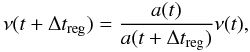 (1)where
a(t) is the expansion factor of the Universe.
(1)where
a(t) is the expansion factor of the Universe.
The treatment of non-thermal electrons produced by X-ray will be described in Sect. 3.5
2.2. Helium reionization
The intergalactic medium is mainly composed of hydrogen and helium, with contributions of 90% and 10% in number. Until now, we have run simulations with hydrogen only, but including helium is worth studying because the different value of the ionization thresholds and photoionization rates could affect the reionization history. We included He, He+, and He++ in LICORICE, and used Cen (1992) and Verner et al. (1996) for various cooling rate and cross sections. When helium chemistry is turned on, the ionization fractions (H+, He+ and He++) and the temperature are integrated explicitly using the adaptive scheme described in Paper I. More details on the numerical methods and a validation tests of the treatment of helium are presented in Appendix.
3. Source model
3.1. Computing the star formation rate
Our new source model needs the star formation rate for all baryon particles. We recompute the star formation in the radiative transfer simulations rather than to rerun the dynamical simulation. Here is why and how.
We adopted the procedure described in Mihos &
Hernquist (1994), employing a local Schmidt law and an hybrid-particles algorithm
to implement it in our code. Indeed, in our model, the star formation rate solely depends
on the density, and we make the assumption that the star formation feedback (kinetic and
thermal) on the dynamics does not vary much from the fiducial simulation. LICORICE uses
the classical Schmidt law: 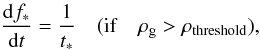 (2)where
t ∗ is defined by:
(2)where
t ∗ is defined by:
 (3)ρg
is the gas density and f ∗ is the star fraction. We set the
parameters t0 ∗ and ρthreshold so
that the evolution of the global star fraction follows closely that of the S20 simulation
(20 h-1 Mpc) in Paper I, and reionization completes at
z ~ 6. In this way, we reuse the tuning made for the S20
simulation, and at high z, we get a similar star formation history as in
the higher resolution (but smaller box size) S20 simulation. All simulations in the
present work have a 100 h-1 Mpc box size. Following the
above equations, a gas particle whose local density exceeds the threshold
(ρthreshold = 5ρcritical × Ωb)
increases its star fraction, f ∗ , where
ρcritical is the critical density of the universe and
Ωb is the cosmological baryon density parameter.
(3)ρg
is the gas density and f ∗ is the star fraction. We set the
parameters t0 ∗ and ρthreshold so
that the evolution of the global star fraction follows closely that of the S20 simulation
(20 h-1 Mpc) in Paper I, and reionization completes at
z ~ 6. In this way, we reuse the tuning made for the S20
simulation, and at high z, we get a similar star formation history as in
the higher resolution (but smaller box size) S20 simulation. All simulations in the
present work have a 100 h-1 Mpc box size. Following the
above equations, a gas particle whose local density exceeds the threshold
(ρthreshold = 5ρcritical × Ωb)
increases its star fraction, f ∗ , where
ρcritical is the critical density of the universe and
Ωb is the cosmological baryon density parameter.
3.2. Limiting the number of sources
We compute the increase in the star fraction for each particle, Δf ∗ between two consecutive snapshots. Then the total mass of young stars formed in a particle is m × Δf ∗ , where m is the mass of the particle. To avoid a huge number of sources, we had to set a threshold on the new star fraction for the particle to act as a source. We used Δf ∗ > 0.001. We checked that this leaves out a negligible amount of star formation, about 0.4%. It happens that several source particles reside in the same radiative transfer cell, but we treated individually ray tracing for each source.
3.3. Choosing an IMF
With our mass resolution, this amount mgas × Δf ∗ corresponds to a star cluster or a dwarf galaxy so an IMF should be taken into account. We choose a Salpeter IMF, with masses in the range 1.6−120 M⊙ or 100−120 M⊙ (model S2). The first range is used to model the SED of an intermediated Pop II and Pop III star population, and the other one is for pure Pop III stars.
3.4. Computing the luminosity and SED of the stellar sources
The next step is to make the link between the amount of created stars and the luminosity of the sources. When only the ionizing UV luminosity is considered, it is quite justified to use simple models. For example we can make it proportional to the mass of the host dark matter halo (Iliev et al. 2006b), or, as we did in Paper I, to the mass of the baryonic particles newly converted into stars. Things are more complicated when we consider both the Lyman band and ionizing UV. Indeed, since each particle is massive enough to contain a representative sample of the choosen IMF, and since each mass bin has a different life time, we should consider an SED evolving with the age of the star particle. This would be possible using pre-tabulated SEDs. However, unlike in Paper I, we decided to use hybrid particles which begin to produce photons as soon as a small fraction of the particle is turned into stars. This is useful to make the local luminosity less noisy in the early EoR when the source mass resolution is an issue. Including this star formation history for each particle and convolving with the time-varying SED would be extremely costly in terms of both memory and computation time.
We simplified the issue by considering the fact that in the Lyman and UV band, most of the luminosity is produced by the massive stars, with a short life time comparable to the time between two snapshots of our simulations. So we decided to use a constant SED and luminosity during a characteristic life time. Both luminosity and SED are computed independently in each of the Lyman and ionizing band. To compute the luminosity and the SED for a star particle we use the data for massive, low metallicity (Z = 0.004 Z⊙) stars in the main sequence (Meynet & Maeder 2005; Hansen & Kawaler 1994, see Table 2). The details of how this is done can be found in Appendix. The constant luminosity and characteristic life time, computed in the two spectral bands, are given in Table 3 We find characteristic life time of <8 Myr for the UV band. In the implementation of the UV transfer however, for technical reasons, the source fraction of the particle actually shines for a duration equal the interval between two snapshots. This varies varies between 6 and 20 Myr, so we recalibrate the luminosity to produce the correct amount of energy. The whole point of the procedure, is to take the different typical life time in the Lyman band into account, especially at at z, when Lyman-α coupling is not yet saturated. We should not concentrate the emission within a single snapshot interval, which is 3 times shorter than the source life-time, or we would artificially boost the coupling between the spin temperature of hydrogen and the kinetic temperature of the gas and alter the resulting brightness temperature. Consequently we let each newly formed star fraction of a particle shine for 3 consecutive snapshots, which is close to the typical life time in the Lyman band, and we still recalibrate the luminosity to produce the correct amount of energy. While we do not use a time-evolving SED, we believe that implementing different life times for the Lyman and UV sources with the correctly average luminosities is a substantial improvement in our source model.
We use an escape fraction fesc = 0.12 for photoionizing UV photons and fesc = 1 for Lyman-α.
Physical properties of low metalicity (Z = 0.004 Z⊙) main sequence stars (Meynet & Maeder 2005).
Averaged luminosities and life times of our source model for a baryon particle depending on the energy band.
3.5. X-ray source model
X-rays can have a significant effect on the 21 cm brightness temperature. The X-ray photons, having a smaller ionizing cross-section, can penetrate neutral hydrogen further than UV photons and heat the gas above the CMB temperature. This X-ray heating effect on the IGM is often assumed to be homogeneous because of X-rays’ long mean free path. In reality, the X-ray flux is stronger around the sources and the inhomogeneous X-ray flux can bring on extra fluctuations for the 21 cm brightness temperature (Pritchard & Furlanetto 2007; Santos et al. 2008). Moreover, patchy reionization induce further fluctuations in the local X-ray flux which can only be accounted for using a full radiative transfer modeling.
X-rays luminosity
First, we need to determine the luminosity and location of X-rays sources. We simply divided the total luminosity, Ltot, of all source particles into a stellar contribution, Lstar, and a QSO contribution, LQSO. LQSO depends on the star formation rate, since Ltot itself is proportional to the increment of the star fraction, Δf ∗ , between two snapshots of the dynamic simulation.
One reason for this approach is that X-ray binaries and supernova remnants contribute to X-ray sources as well as quasars and they are strongly related to the star formation rate. Following the work of Glover & Brand (2003), we took 0.1% of Ltot as the fiducial X-ray source luminosity, LQSO. However, considering that they assumed a simple and empirically motivated model we have also run simulations with different values LQSO, 1% and 10% of Ltot. Quasar luminosity fractions less than 0.1% are not of interest for us, since their heating effect will be negligible.
X-ray energy range and nature of the sources
First, we have to choose the photon energy range since hard X-ray photons have a huge
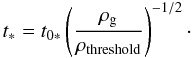
mean free path which costs a lot for ray-tracing computations. The comoving mean free path
of an X-ray with energy E is (Furlanetto
2006)  (4)Only photons with
energy below
(4)Only photons with
energy below ![$E\sim 2[(1+z)/15]^{1/2}\overline{x}^{1/3}_{\rm{HI}}\,$](/articles/aa/full_html/2010/15/aa14347-10/aa14347-10-eq96.png) keV are absorbed within a
Hubble time and the E-3 dependence of the cross-section means
that heating is dominated by soft X-rays, which do fluctuate on small scales (Furlanetto
et al. 2006). Therefore, we choose an energy range for X-ray photons from 0.1 keV to
2 keV. The photons with energy higher than 2 keV are not absorbed until the end of
simulation at z ≈ 6.
keV are absorbed within a
Hubble time and the E-3 dependence of the cross-section means
that heating is dominated by soft X-rays, which do fluctuate on small scales (Furlanetto
et al. 2006). Therefore, we choose an energy range for X-ray photons from 0.1 keV to
2 keV. The photons with energy higher than 2 keV are not absorbed until the end of
simulation at z ≈ 6.
While the most likely astrophysical sources of X-ray during the EoR are supernovae, X-binaries and (mini-) quasars, it is interesting to mention that the X-ray SED of supernovae and X-binaries typically peaks above 1 keV (e.g. Oh 2001). This means that most of the X-rays emitted by these sources will interact with the IGM more than 108 years later, which is not true for QSO-like SEDs. During this time interval the global source mass (and, to first order, luminosity) easily rises by a factor of 10. Thus the longer delay will lower the effective luminosity of X-binaries and supernovae compared to QSO. For this reason, but also to avoid detailed modeling of some aspects while others, like the overall luminosity of X-ray sources, remain largely unconstrained, we use QSO as our typical X-ray source.
QSO spectral Index
We model the specific luminosity of our QSO-like sources as a power-law with index
α;  (5)k
is a normalization constant so that
(5)k
is a normalization constant so that 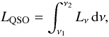 (6)where
hν1 = 0.1 keV and
hν1 = 2 keV. The amount of X-ray heating
can be altered by the shape of the spectrum but there exists a large observational
uncertainty in the mean and distribution of α. We extrapolate from the
measurement of extreme UV spectral index by Telfer et al.
(2002) to higher energy. The index values are derived from fitting
1Ry < E < 4Ry, and we
extrapolated to 2 keV. The measured value by Telfer et al.
(2002) is approximately ≈ 1.6, but with a large gaussian standard deviation of
0.86. Scott et al. (2004) derived an average value
of α = 0.6 from a sample of FUSE and HST quasars. We choose
α = 1.6 as our fiducial case, and used α = 0.6 for
comparison.
(6)where
hν1 = 0.1 keV and
hν1 = 2 keV. The amount of X-ray heating
can be altered by the shape of the spectrum but there exists a large observational
uncertainty in the mean and distribution of α. We extrapolate from the
measurement of extreme UV spectral index by Telfer et al.
(2002) to higher energy. The index values are derived from fitting
1Ry < E < 4Ry, and we
extrapolated to 2 keV. The measured value by Telfer et al.
(2002) is approximately ≈ 1.6, but with a large gaussian standard deviation of
0.86. Scott et al. (2004) derived an average value
of α = 0.6 from a sample of FUSE and HST quasars. We choose
α = 1.6 as our fiducial case, and used α = 0.6 for
comparison.
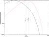 |
Fig. 1 Normalized spectral intensity of our source model. Black solid line is the SED from Salpeter IMF and red dashed line is from top-heavy IMF. |
Secondary Ionization
X-rays deposit energy in the IGM by photoionization through three channels. The primary high velocity electron torn from hydrogen and helium atoms distributes its energy by 1) collisional ionization, producing secondary electrons, 2) collisional excitation of H and He and 3) Coulomb collision with thermal electrons. The fitting formula in Shull & van Steenberg (1985) is used to compute the fraction of secondary ionization and heating. These are taken into account when computing the evolution of the state of the IGM.
Then, it is legitimate to ask whether the lyman-α electrons resulting from the collisional excitations are important for the Wouthuysen-Field effect. The simple answer is that, in our choice of models, the energy emitted as X-ray is at most 10% of the UV energy, itself 3 times less than the Lyman luminosity. Moreover at most 40% of the X-ray energy is converted into excitations (Shull & van Steenberg 1985), and only ~30% of the excitations result in a Lyman-alpha photon (Pritchard & Furlanetto 2006). So, in the best case, Lyman-α photons produced by X-ray represent only 0.3% of the photons produced directly by the sources.
4. Results
4.1. Ionization fraction
The evolution of the averaged ionization fraction tells us about the global history of reionization. We plot the mass and volume weighted average ionization fraction in Fig. 2. Including quasar (S4, S5, S6 and S7, not plotted) does not change the global evolution of the ionization fraction much, because of its small fraction of the total luminosity. The total number of emitted photons is similar to S1. The S3 simulation has also the same number of emitted photons, but S3 reaches the end of reionization a little bit earlier (Δz ≈ 0.25) than S1. Unlike other simulations, S3 contains helium which occupies 25% of the IGM in mass. Including helium, the total number of atoms is reduced by 20%. At the same time, unless X-ray are the dominant source of reionization, most of the helium is only ionized once while z > 6, due to the higher energy threshold for the secondary ionization(He++). Therefore the number of emitted photons per baryon is higher in S3 than S1, and it results in an earlier reionization.
On the other hand, S2 has the same number of photon absorbers as S1, but the total number of emitted photons is much higher than in S1. Using a top-heavy IMF, it produces 10 times more photons (see Fig. 1 and Table 3), and results in a Δz ≈ 1 earlier reionization.
In all three cases, volume weighted values are less than mass weighted values, since gas particles in dense regions around the sources are ionized first. The volume occupied by each particle is estimated using the SPH smoothing length.
We computed the Thomson optical depth for all simulations, the values are τ = 0.062, 0.076, 0.064 for S1, S2 and S3. The other simulations (S4-S5) have the same τ as S1, since they follow the same evolution of ionization fraction. They are somewhat lower than the Thompson optical depth derived from WMAP5 (Hinshaw et al. 2009), τ = 0.084 ± 0.016, only the S2 value is within 1σ of the WMAP5 value. A variable escape fraction, decreasing with time, would allow the IGM to start ionization earlier and increase τ, without terminating ionization after z = 6.
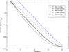 |
Fig. 2 Mass (thicker lines) and volume (thinner lines) weighted ionization fraction of hydrogen. S1 and S3 use Salpeter IMF and S2 use top-heavy IMF. S3 contains helium element. |
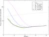 |
Fig. 3 The evolution of the gas temperature of the neutral IGM with redshift. The neutral gas is chosen so that its ionization fraction is less than 0.01. |
4.2. Gas temperature
The main goal of this study is to investigate the effect of inhomogeneous X-ray heating on the 21-cm signal. If the Ly-α coupling is sufficient, and X-rays can heat the gas above the CMB temperature TCMB, the 21-cm signal will be observed in emission. However if the X-ray heating is not very effective, particularly during the early phase of the EoR, we will observe the signal in absorption.
We plot in Fig. 3 the averaged gas temperature of the neutral IGM whose ionization fraction xHII is less than 0.01. We chose the criterion of xHII < 0.01 for the following reasons. Once a gas particle is 10% ionized, it is heated by photoheating to a temperature of several thousand Kelvin. At redshift 10, the number of gas particles which have an ionization fraction between 0.01 and 0.1 is only 0.1% of all the particles, but if we include these particles, the average temperature increases from 2.94 K to 5.41 K. Therefore, we used the criterion xHII < 0.01 to evaluate properly the average temperature of neutral regions, and verified that xHII < 0.001 gives a very similar average temperature. We have checked that even for model S7 which has the highest level of X-rays, at z > 7.5, 99% of the neutral IGM has indeed an ionization fraction less than 1%, so we have not excluded a significant fraction of the 21 cm emitting IGM from our average. This neutral gas is mostly located in the voids of the IGM. In fact, we have to consider Ly-α heating as well as X-ray heating since a few K difference can reduce the intensity of δTb by up to 100 mK. We recompute the gas temperature to include Ly-α heating as a post-treatment using the formula from Furlanetto & Pritchard (2006). This was detailed in Paper I. The temperature of all simulations in Fig. 3 decreases until z ≈ 12 because of the adiabatic expansion of the universe. Then S7, which has the highest LQSO, starts to increase first and reaches the CMB temperature at redshift z ≈ 8.8. Our fiducial model, S4, which contains 0.1% of total energy as X-rays, shows very little increase with respect to S1, a simulation without X-rays. Even for S7, the gas temperature of neutral hydrogen in the void is still under the TCMB until z ≈ 8.8. This means that the X-ray heating needs time to heat the IGM above TCMB. Even with a rather high level of X-ray, the absorption phase survives and produces greater brightness temperature fluctuations than the subsequent emission phase (the delay in the absorption of X-ray connected to the long mean free path is partly responsible for this). It will be important to keep this result in mind when choosing the design and observation strategies for the future instruments.
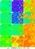 |
Fig. 4 Differential brightness temperature maps for different simulations. The thickness of the slice is ≈ 2 Mpc. The maps in the left column are when ⟨ xα ⟩ = 1, the middles when ⟨ xα ⟩ = 10 and the right when ⟨ xHII ⟩ = 0.5. The black contour separates absorption and emission region. (l) shows no absorption region. |
There is a large observational uncertainty in the mean and distribution of the quasar spectral index α. Our fiducial model assumes α = 1.6 but we run a simulation (S5) with α = 0.6 for comparison. The total emitted energy is fixed, but the S5 simulation has more energetic photons which penetrate the ionization front further than those of S4. However, the difference of the gas temperature between two simulations is negligible. The temperature of S5 is slightly higher than S4, but the difference is less than 0.5 K at all redshifts.
We estimate that our 1% model yields around 5 times more X-rays than the fiducial model in Santos et al. (2008), although the source formation modeling is quite different and the comparison is difficult (we do not use the dark matter halo mass at all in computing the star formation rate). However, comparing their plots of the average temperature and ionization fraction evolution with ours, we can deduce that their average gas kinetic temperature rises above the CMB temperature around ionization fraction xHII = 10% while in our case the same event occurs at xHII = 15%. We find several reasons for this apparent discrepancy. First we defined neutral IGM as xHII < 0.01 and use this to compute the average gas temperature. Although this is not absolutely explicit in the paper, we believe they use xHII < 0.5, thereby including warmer gas in the average. Then, they have a more extended reionization history, which reduces the effect of the delay in the X-ray heating (see next section). Finally the initial X-ray heating is shifted to higher redshifts, when the difference between the average neutral gas temperature and the CMB temperature is less.
4.3. Brightness temperature maps
We have run Lyman-α simulations as a further post-treatment to obtain
the differential brightness temperature δTb.
The δTb is determined by various elements,
and it is expressed as (Madau et al. 1997):
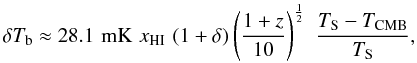 (7)where
δ is the baryon over density, Ts is the
spin temperature, TCMB is the CMB temperature, and
xHI is the neutral fraction. The contribution of the
gradient of the proper velocity is not considered in this work.
(7)where
δ is the baryon over density, Ts is the
spin temperature, TCMB is the CMB temperature, and
xHI is the neutral fraction. The contribution of the
gradient of the proper velocity is not considered in this work.
The spin temperature Ts can be computed with: 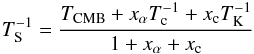 (8)and
 (9)where
Pα is the number of
Lyman-α scatterings per atom per second,
A10 is the spontaneous emission coefficient of the 21 cm
hyperfine transition, T ⋆ is the excitation
temperature of the 21 cm transition, and C10 is the
deexcitation rate via collisions. Details on deriving these relations and computing
C10 can be found, e.g., in Furlanetto et al. (2006). The peculiar velocity gradients (Barkana & Loeb 2005; Bharadwaj
& Ali 2004) is not considered in this work.
(9)where
Pα is the number of
Lyman-α scatterings per atom per second,
A10 is the spontaneous emission coefficient of the 21 cm
hyperfine transition, T ⋆ is the excitation
temperature of the 21 cm transition, and C10 is the
deexcitation rate via collisions. Details on deriving these relations and computing
C10 can be found, e.g., in Furlanetto et al. (2006). The peculiar velocity gradients (Barkana & Loeb 2005; Bharadwaj
& Ali 2004) is not considered in this work.
As we can see in Eq. (9), TS is coupled to the CMB temperature TCMB by Thomson scattering of CMB photons, and to the kinetic temperature of the gas TK by collisions and Ly-α pumping. Coupling by collisions is efficient only at z > 20, or in dense clumps, so Ly-α is the key coupling process in the diffuse IGM. The δTb maps are a good way to see how these different elements affect the signal. In Fig. 4 we show several δTb maps of the same slice from different radiative transfer simulations, S1, S2, S6 and S7. S4 and S5, which sets the X-ray luminosity at 0.1% of the UV luminosity show a trend very similar to S1 and are not plotted. The bandwidth of the slice is 0.1 MHz for all maps, which corresponds to 1.9 Mpc for the maps on the left column (a)–(d), 1.8 Mpc for (e)–(h) and 1.6 Mpc for (i)–(l).
The left four maps of δTb in Fig. 4a–d, are plotted when the mass averaged Ly-α coupling coefficient xα is ⟨ xα ⟩ = 1. This value is interesting because in this moderate coupling regime, fluctuations in the Ly-α local flux induce fluctuations in the brightness temperature, which is not the case anymore when the coupling saturates. The corresponding redshifts are z = 10.50 for S2 and 10.13 for the others. The corresponding averaged ionization fractions are 0.005, 0.018, 0.005 and 0.005 for (a)–(d). Indeed, the averaged ionization fraction of S2 is higher than the others since it uses a harder spectrum. The ratio of the integrated energy emitted in the Lyman band (Ly-α < E < Ly-limit) with respect to the ionizing band, β = ELyman/Eion, is three times less for S2 than for the others. For a given number of emitted Ly-α photons, a harder spectrum produces a larger number of UV ionizing photons, therefore S2 has a higher ionization fraction when ⟨ xα ⟩ = 1. S1 shows a deeper absorption region around the ionized bubbles than S2, and it is also due to the different ratio of the number photons in the Lyman band and the ionizing band. In the case of S1, the ionized bubble is smaller than the highly Ly-α coupled region. Since the kinetic temperature outside of ionized bubble is a few kelvin, which is lower than the CMB temperature (TCMB ≈ 30K), the neutral hydrogen has a strong 21-cm absorption signal. On the other hand, the highly Ly-α coupled regions in S2 mostly resides in the ionized bubbles, which are bigger than in S1. S7 has almost the same averaged ionization fraction and ionized bubble size as S1, but the gas around the ionized bubbles as well as in the void is heated by strong X-rays. The signal is still in absorption because the X-ray heating has not been able to raise the IGM temperature above TCMB, but the intensity is reduced. Contrary to S1 and S2, the neutral gas around the ionized bubbles produces a weaker signal than in the void, because the gas around the bubbles is more efficiently heated by X-rays. S6 shows an intermediate behavior between S1 and S7.
The four maps in the middle of Fig. 4e–h, are for ⟨ xα ⟩ = 10. The corresponding redshifts are z = 9.03 for S2 and 8.57 for the others. The averaged ionization fractions are 0.043, 0.141, 0.043 and 0.040 for (e)–(h). These redshifts when ⟨ xα ⟩ = 10 are interesting because the amplitude of fluctuation δTb reaches a maximum. If we do not consider the effect of Ly-α coupling and assume Tk ≫ TCMB, which does not allow the signal in absorption, the largest fluctuations would appear around ⟨ xHII ⟩ = 0.5 as noticed by Mellema et al. (2006a) and Lidz et al. (2007a), but including the inhomogeneous Ly-α coupling and computing TK self-consistently, this maximum is shifted to an earlier phase of reionization. The ionization fraction and bubble size in S2 are still greater than in the other models, but the absorption intensity is lower than in S1. Here is why. The evolution of kinetic temperature in the void regions is dominated by the adiabatic cooling: the temperature drops as the expansion progresses. The kinetic temperature of S1 in the voids is lower than in S2 by 0.5 K due to the difference in redshift, which explains the stronger absorption intensity in S1. The neutral gas around ionized bubbles in S7 is heated by the high X-rays level above TCMB, and starts to produce the signal in emission. The neutral gas in the voids is also affected by X-rays. However, it is not sufficiently heated yet so that the signal turns everywhere from absorption to emission. Nevertheless the intensity of the signal is reduced by the X-ray heating, and it shows the weakest signal among the four maps at ⟨ xα ⟩ .
The four maps on the right of Fig. 4, (i)–(l), are for ⟨ xHII ⟩ = 0.5. The corresponding redshifts are z = 7.68 for S2, 7.00 for S1 and S6, 6.93 for S7. The averaged Ly-α coupling coefficients, xα, are 138.3, 34.9, 138.75 and 187.75 for (i)–(l). Contrary to the above cases, the absorption intensity of S1 in the void region is weaker than that of S2. This is due to the Ly-α heating. Ly-α heating is negligible during the early phase, but the amount of Ly-α heating accumulated between z ~ 12 and z ~ 7 can heat the gas in the voids by several kelvins. In order to reach 50% ionization, S1 produces a larger number of Ly-α photons, which propagate beyond the ionizing front. The ⟨ xα ⟩ of S1 is almost 4 times greater than that of S2, and the accumulated Ly-α heating increases the kinetic temperature by 3–4 K more than in S2. The intensity in absorption is very sensitive to the value of kinetic temperature, so this small amount of heating reduces the signal by up to 100 mK. The X-ray heating in S7 is strong enough to heat all the gas above TCMB at this redshift, so we see the signal in emission everywhere. S6 shows intermediate features between S1 and S7, showing the weakest signal. Indeed, the X-ray heating in S6 increased the gas temperature in the neutral voids just around the TCMB, which is the transition phase from absorption to emission.
4.4. Power spectrum
Figure 5 shows 3 dimensional power spectra of the
brightness temperature fluctuations for the S1, S2, S6 and S7 simulations. The power
spectrum can be defined as the variance of the amplitude of the Fourier modes of the
signal for a given wavenumber modulus:
 (10)We binned our modes
with
(10)We binned our modes
with  and plotted
the quantity
Δ2 = k3P(k)/2π2.
The power spectra of S4, S5 are not presented in Fig. 5 since their patterns are similar to S1. During the early phase, when
⟨ xα ⟩ = 1, the amplitude of the
powerspectrum of 4 simulations are similar. The spectra follow patterns similar to the
power spectrum of S100 in Paper I (see Fig. 15). Model S6, shows a spectrum similar to the
fiducial model of Santos et al. (2008). The main
difference in shape appears at k > 1 h-1Mpc in our
model. This is possibly connected to the fact that they assume a
and plotted
the quantity
Δ2 = k3P(k)/2π2.
The power spectra of S4, S5 are not presented in Fig. 5 since their patterns are similar to S1. During the early phase, when
⟨ xα ⟩ = 1, the amplitude of the
powerspectrum of 4 simulations are similar. The spectra follow patterns similar to the
power spectrum of S100 in Paper I (see Fig. 15). Model S6, shows a spectrum similar to the
fiducial model of Santos et al. (2008). The main
difference in shape appears at k > 1 h-1Mpc in our
model. This is possibly connected to the fact that they assume a  dependence of
the Lyman-α flux, while at short distances from the sources (<10
comoving Mpc), wings scattering effects produce a
dependence of
the Lyman-α flux, while at short distances from the sources (<10
comoving Mpc), wings scattering effects produce a  dependence (Semelin et al. 2007). Also noticeable
is the difference between S6 and S7. S7 is depleted at small scale, the strong X-ray
heating damping the absorption near the sources. On very large scale, however the already
strong heating in S7 creates temperature fluctuations which boost the S7 power spectrum.
dependence (Semelin et al. 2007). Also noticeable
is the difference between S6 and S7. S7 is depleted at small scale, the strong X-ray
heating damping the absorption near the sources. On very large scale, however the already
strong heating in S7 creates temperature fluctuations which boost the S7 power spectrum.
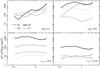 |
Fig. 5 Power spectrum evolution of the δTb from the S1 (thin black), S2 (thick black), S6 (thin gray) and S7 (thick gray) simulations. S2 use top-heavy IMF whereas the others use Salpeter IMF. S6 has 1% and S7 has 10% of total luminosity for X-rays. |
When ⟨ xα ⟩ = 10, the power of both S6 and S7 decreases since X-ray heating prevents a strong absorption signal. The strong X-ray heating of S7 increases the gas temperature around TCMB, and it shows the smallest power. However, the power of S6 falls down under the power of S7 when the hydrogen is 50% ionized. At this redshift, the rising temperature of neutral gas reaches TCMB in S6, while it is already much greater than TCMB in S7. This is also visible in Fig. 4. Later, when ⟨ xHII ⟩ = 0.9, all power spectra drop. Our S6 model agrees quite well with Santos et al. (2008) both in shape and amplitude for these two last stages. Indeed both the effects of Lyman-α coupling and X-ray heating reach a saturation in the determination of the brightness temperature, erasing the differences in our treatments. S2 has the largest power over all scale when ⟨ xHII ⟩ = 0.5 and ⟨ xHII ⟩ = 0.9. This is due to the near lack of Ly-α heating. Let us mention however that some sort of transition to Pop II formation should have occurred by then, providing some level of Ly-α heating. So S2 is probably not realistic during the late EoR.
In brief, the 21-cm power spectra of our models vary in the 10 to 1000 mK2 range, in broad agreement with Santos et al. (2008) who included the inhomogeneous X-ray and Ly-α effect on the signal in a semi-analytical way, with moderate discrepancies at high-redshift and small scale due to wing effet in the Lyman-α radiative transfer. Quite logically our results differ at high-redshift from (Mellema et al. 2006b; Zahn et al. 2007; Lidz et al. 2007b; McQuinn et al. 2006) who focused on the emission regime. These authors found a flattening of the spectrum around ⟨ xHII ⟩ = 0.5. It is interesting to notice that in the case of a strong X-ray heating (model S7) the spectrum is quite flat at all redshift (temperature fluctuation boost the power on large scales at high-redshift). In the future observations, this would be a first clue of larger-than-expected contribution from X-ray sources.
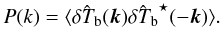
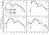 |
Fig. 6 Evolution of the brightness temperature power spectrum with redshift. k = 0.07 h/Mpc (thin black), k = 0.19 h/Mpc (thick black ), k = 1.00 h/Mpc (thin gray) and k = 3.15 h/Mpc (thick gray). |
We now plot the evolution of the power as a function of redshift for 4 different k values. The evolution of the power spectrum with and without X-rays is very different. S1 and S2, which do not have X-rays, show a single maximum on small scales (k = 1.00 h/Mpc and k = 3.15 h/Mpc) around redshifts 8.5 and 9 which correspond to the redshifts of ⟨ xα ⟩ = 10 for each simulation. On large scales (k = 0.07 h/Mpc and k = 0.19 h/Mpc) the power spectrum shows two local maxima on large scale. The first peak is related to the Ly-α fluctuations. The δTb fluctuations are dominated by Ly-α fluctuations at high-redshift, but it decreases when the Ly-α coupling saturates. Then it rises again. This time, the fluctuations are dominated by the fluctuations of ionization fraction. The second peak appears at the redshift when ⟨ xHII ⟩ = 0.5 for each simulations. The overall amplitude of S1 and S2 are similar, but the position of the local maximum peaks of S2 are at higher redshift due to the faster reionization. The key to the single-double peak difference is that the contribution of the ionizing field fluctuation to the brightness temperature power spectrum increases during reionization on large scale but not on small scales (Iliev et al. 2006b).
 |
Fig. 7 The evolution of the 21-cm PDF. The redshifts are 14.05, 10.64 and 8.48 for a), b), and c). The PDFs of panel d) is chosen so that the ionization fraction is 0.5. The red curves on b) are gaussian fits with the mean and variance of the PDFs. |
With X-rays (models S6 and S7), the evolution follows a different scenario. We find a pattern similar to Santos et al. (2008). On small scales (thin and thick gray in Fig. 6), the intensity of the signal increases up to the maximum as the spin temperature couples to the kinetic temperature. Then it decreases during the absorption-emission transition. As the fluctuation due to the ionization fraction comes to dominate, the power reincreases slightly or remains in a plateau until it drops at the end of reionization. The evolution of the power on small scale does not show a marked minimum. The evolution of large scales (thin and thick gray in Fig. 6) is the most interesting: it shows three maxima. From high-redshift to low redshift, each peak corresponds to the period where the fluctuation of the Ly-α coupling, gas temperature and ionization fraction dominate. There exists a deep suppression between the second and the third peaks which does not appear without X-ray. It occurs when the X-ray heating raises the gas temperature of the neutral IGM around TCMB, which dampens the signal. The second minimum in S7 occurs earlier than in S6, since the stronger X-ray heating of S7 increase the gas temperature around TCMB at a higher redshift. We find a much narrower third peak in S4 (not plotted), which uses a 10 times weaker X-ray heating than S6. The position and amplitude of the peaks as well as the width depend on the intensity of X-ray heating. The width of the third bump (6.5 < z < 7.5) is the largest in S7 (with 10% X-ray) and the smallest or negligible in S4 (with 0.1% X-ray). The existence/position of this third peak and of the second dip in the evolution of large scale power spectrum will be measurable by LOFAR and SKA observations, and it will help us constrain the nature of the sources during the EoR.
4.5. Non-Gaussianity of the 21-cm signal
The non-gaussianity of the 21-cm signal has been studied in previous works. Ciardi & Madau (2003); Mellema et al. (2006b) shows the non-gaussianity of the 21-cm signal in numerical simulations by computing the pixel distribution function (PDF). Ichikawa et al. (2010) draws the history of reionization from the measurement of the 21-cm PDF. Harker et al. (2009) compute the skewness of the PDF and show how it could help in separating the cosmological signals from the foregrounds. However, all these works model the signal in emission only.
We present the 21-cm PDF from our simulations in Fig. 7, for several representative redshifts. To obtain the 21-cm PDF, we sample δTb within a 1 h-1 Mpc resolution, an acceptable value for SKA. The 21-cm PDF from our simulations is highly non-Gaussian as expected, but is also quite different from Ciardi & Madau (2003); Mellema et al. (2006b); Harker et al. (2009) and Ichikawa et al. (2010), Our distributions extend to negative differential brightness temperature with a variety of shapes depending on the redshift.
The panel (a) of Fig. 7 is the 21-cm PDF at the beginning of reionization, z = 14.05. It is at the beginning of reionization that Ichikawa et al. (2010) find a 21-cm PDF closest to a Gaussian, but this is also when their model is the less relevant. In our case, all signals are found in absorption and their distribution is peaked around 0mK, completely non-Gaussian.
We show the PDFs at z = 10.64, still during the early EoR, in panel (b) of Fig. 7. The position of peaks are shifted around −100 mK ~ −50 mK which means that the spin temperature of the particles is decoupled from TCMB by Ly-α photons. The PDF is much close to a gaussian distribution, extending to positive values (the smooth curves are the best gaussian fit to the PDFs). However, all of them are left skewed (toward negative temperature). The reason for this negative skewness is the same as the reason for the positive skewness in Mellema et al. (2006b); Ichikawa et al. (2010); Harker et al. (2009): it is due to the signal from high density regions seen in absorption for us and in emission for them.
Panel (c) in Fig. 7 shows the PDFs when z = 8.48. Here we find a bimodal distribution with a plateau in the absorption region between 100 mK and 0 mK, for models S1, S2 and S4. The left peaks of the PDFs moves also toward higher δTb with increasing heating efficiency. In the case of S7, the left peak merges with the right one, and the form is very similar to a gaussian.
The panel (d) of Fig. 7 is plotted when the ionization fraction is 50%. The width of the PDF of S1 and S4 is reduced because Ly-α heating is well advanced. We find signals in emission in S6 and S7, since X-rays heat the gas in neutral regions above TCMB. Indeed, these PDF forms are similar to Ichikawa et al. (2010). The PDFs of S6 and S7 could be fitted by the Dirac-exponential-Gaussian distribution used by Ichikawa et al. (2010). S2 has broad PDF still, since the Ly-α heating is 4 times lower than in the others and it retains the signal in strong absorption.
It is interesting to note that the PDF always shows a spike around ~0 mK. During the beginning of reionization, it is due to the large amount of neutral hydrogen whose spin temperature is still well coupled to the CMB temperature. As the reionization proceed, the spin temperature is decoupled from the CMB and the number of pixels at ~0 mK decreases, but the peak grows again with the increasing contribution from completely ionized regions. This feature is interesting since interferometers such as LOFAR or SKA only measure fluctuations in the signal and do not directly provide a zero point.
Ichikawa et al. (2010) extract informations about the averaged ionization fraction from the 21-cm PDF. As could be expected our PDFs converge with their result when the contribution from X-ray sources is sufficient and the EoR somewhat advanced. What we find is that a clear tracking of the nature of the ionizing source remains on the PDF when the absorption phase is modeled. A strong X-ray contribution produce unimodal PDFs while a weak X-ray contribution yield a bimodal PDF.
The evolution of the skewness is presented in Fig. 8. The skewness γ is defined as
![\begin{equation} \gamma=\frac{\frac{1}{N}\Sigma _i (\delta T_{\rm b}^i -\overline{ \delta T_{\rm b}})^3 } {[\frac{1}{N}\Sigma _i (\delta T_{\rm b}^i -\overline{\delta T_{\rm b}})^2]^{3/2}} , \end{equation}](/articles/aa/full_html/2010/15/aa14347-10/aa14347-10-eq181.png) (11)where N
is total number of pixels in δTb data cube,
(11)where N
is total number of pixels in δTb data cube,
 is
δTb in ith pixel, and
is
δTb in ith pixel, and
 is
the average on the data cube.
is
the average on the data cube.
At the beginning the skewness is highly negative for all simulations as we can expect the skewness rises to a local positive maximum when the average ionization fraction is a few percents. It is interesting to notice that the skewness of all simulations close to zero again when the neutral fraction is about 0.3. While this behavior could be used to provide a milestone of reionization, its robustness should first be checked. We can notice that two of the three models presented in Harker et al. (2009) show the same behavior. Those are however the two less detailed models.
Another interesting feature in Fig. 8 is that the skewness of S7 has two local maxima while others do not. Again, this could be used as a clue to a large contribution from X-ray sources.
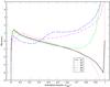 |
Fig. 8 Evolution of the skewness with the ionization fraction. |
5. Conclusions
We modeled the 21-cm signal during the EoR using numerical simulations putting the emphasis on how various types of sources can affect the signal. The numerical methods used in this work are similar to Baek et al. (2009). The N-body and hydrodynamical simulations have been run with GADGET2 and post-processed with UV continuum radiative transfer further processed with Ly-α transfer using LICORICE, allowing us to model the signal in absorption. The main difference from the previous work is a more elaborated source model, including X-ray radiative transfer and He chemistry.
We have run 7 simulations to investigate the effect of different IMFs, helium, different spectral indexes and the different luminosities of X-rays sources. The reference simulation in this work, S1, using only hydrogen and stellar type sources, reached the end of reionization at z ≈ 6.5 and showed a strong absorption signal until the end of reionization. Our top heavy IMF (model S2) produces ~2.6 times more ionizing photons than the Salpeter IMF. S2 reached the end of reionization earlier than the others by Δz ≈ 1. In addition the different SED changes the ratio of Ly-α and to ionizing UV photon numbers, and it slows down the saturation of the Ly-α coupling and the heating by Lyman-α in the top heavy IMF case. This modifies the statistical properties of 21-cm signal.
The simulation with helium, S3 also has a slightly earlier reionization than the others since the number of emitted photons per baryon is higher. Except for the slightly lower kinetic temperature in the bulk of ionized regions due to the higher ionization potential than for hydrogen, the properties of the 21-cm signal from S3 is similar to S1. We chose QSO type sources with a power-law spectrum as X-ray sources in model S4 to S7. The spectral index α has large observational uncertainty, so we used two different spectral indexes. S4 and S5 have 0.1% of the total luminosity in the X-ray band. S5 uses α = 0.6, while other simulations with X-rays use α = 1.6. S5 showed very little difference on the gas temperature with respect to S4. S4, S6 and S7 have different luminosities in the X-ray band, keeping the same values for the other simulation parameters. Using a stronger X-ray luminosity indeed increased the gas temperature in the neutral hydrogen. Accordingly the 21-cm signal and its power spectra are modified. We found an increase of a few kelvin for the neutral gas temperature in our fiducial model, S4, in which X-rays account for 0.1% of the total emitted energy. The 21-cm signal in S4 was similar to S1, showing the maximum intensity in absorption, ~200 mK, at z ≈ 9. Stronger X-ray levels increase the gas temperature and reduce the intensity. We found that in S6 and S7, which uses 1% and 10% of the total luminosity for X-rays, the absolute maximum intensity in absorption decreases to ~130 mK and ~80 mK. The 21-cm power spectrum of our work is greater by two or three orders of magnitude than in works focusing on the emission regime (Mellema et al. 2006b; Zahn et al. 2007; Lidz et al. 2007b; McQuinn et al. 2006). However, the results are in broad agreement with the work of Santos et al. (2008), who modeled absorption using semi-analytical methods for X-ray and Lyman-α transfer. We noticed that the 21-cm fluctuation is dominated by Ly-α fluctuations during the early phase, X-rays later (or the gas temperature), and the ionization fraction at the end. This is visible on the evolution of the 21-cm power spectrum with redshift. The 21-cm PDF of our work was different from other work, since we do not assume that the spin temperature Ts ≫ TCMB.
The first most important conclusion from our work is that even including a higher than generally expected level of X-ray, the absorption phase of the 21-cm survives. Its intensity and duration are reduced, but the signal is still stronger than in the emission regime. Heating the IGM with X-rays takes time!
The second important result is that we found three diagnostics which could be used in the analysis of future observations to constrain the nature of the sources of reionization. (i) The first and maybe the most robust is the evolution with redshift of large scale modes (k ~ 0.1 h/Mpc) of the powerspectrum. If reionization is overwhelmingly powered by stars, this evolution should have one local minimum (two local maxima). However, if the energy contribution of QSO is greater than ~1%, a second local minimum (third maximum) appears. The higher the X-ray level, the broader the third peak. (ii) The second simple diagnostic is the bimodal aspect of the PDF which disappears when the X-ray level rises above 1% of the total ionizing luminosity. (iii) Last is the redshift evolution of the skewness of the 21-cm signal PDF. While all other models show a single local maximum at a few percent reionization, a very high level of X-rays (>10% of the total ionizing luminosity) produces a second local maximum appear around 50% reionization.
Modeling the sources in the simulation is complex. It involves taking the formation history, IMF, SED, life time, and more into account. Although detailed models are desirable for the credibility of the results, we believe that the effect in the 21-cm signal can be bundled in 3 quantities. The first is the efficiency: how many photons are produced by atoms locked into a star. This parameter must be calibrated to fit observational constraint: end of reionization between redshift 6 and 7, and Thomson scattering optical depth in agreement with CMB experiment. The two other quantities which contain most of the information are two box-averaged ratios: the energy emitted in the Lyman band to the energy emitted in the ionizing band ratio and the same ionizing UV to X-ray ratio. In this work we explored values of 0.32 (model S2) and 0.75 (all other models) for the former and 0.001, 0.01 and 0.1 for the latter. Once additional physics is included in the simulation and using a higher resolution to account for all the sources, it will be interesting to explore the value of these quantities systematically.
We mentioned in the introduction that the minimum boxsize for reliable predictions of the signal is 100h-1 Mpc. It is important to realize that this value (confirmed by emission regime simulations, e.g., Iliev et al. 2006b) is estimated based on the clustering properties of the sources and applies to the topology of the ionization field. It may be underestimated when we study the early absorption regime, when only the highest density peaks contain sources. Their distribution is the most sensitive to possible non-gaussianities in the matter power spectrum. Moreover, they are distant from each other and, consequently, produce large scale fluctuations in the local flux of Lyman-α and X-ray photons. We intend to extend our investigation to larger box sizes in a future work.
A few final words on additional physics not included in our model. Shock heating from the cosmological structure formation is ignored, but it could have the potential to affect the 21-cm signal by increasing the gas temperature above the CMB temperature. However, it is not sure whether shocks are strong enough in the filaments of the neutral regions to affect the 21-cm signal. Mini-halos (~104−108M⊙) form very early during the EoR and are dense and warm enough from shock heating during virialization to emit the 21 cm signal, but Furlanetto & Oh (2006) find that the contribution of mini-halos will not dominate, because of the limited resolution of the instrumentation. However, shock heating is worth investigating with coupled radiative hydrodynamic simulations with higher mass resolution. Also worth investigating is the effect of including higher Lyman lines in the radiative transfer.
LOw Frequency ARray, http://www.lofar.org
Murchison Widefield Array, http://mwatelescope.org/
Giant Metrewave Radio Telescope, http://www.gmrt.ncra.tifr.res.in
21 Centimeter Array, http://21cma.bao.ac.cn/
Square Kilometre Array, http://www.skatelescope.org/
Available at http://aramis.obspm.fr/~baek/these.pdf
Acknowledgments
This work was realized in the context of the SKADS and LIDAU projects. SKADS, the Design Study of the SKA project, financed by the FP6 of the European Commission, the ANR project LIDAU, financed by the French Ministry of Research.
References
- Abel, T., Norman, M. L., & Madau, P. 1999, ApJ, 523, 66 [NASA ADS] [CrossRef] [Google Scholar]
- Baek, S. 2009, Ph.D Thesis [Google Scholar]
- Baek, S., di Matteo, P., Semelin, B., Combes, F., & Revaz, Y. 2009, A&A, 495, 389 [NASA ADS] [CrossRef] [EDP Sciences] [Google Scholar]
- Barkana, R., & Loeb, A. 2004, ApJ, 609, 474 [NASA ADS] [CrossRef] [Google Scholar]
- Barkana, R., & Loeb, A. 2005, ApJ, 626, 1 [NASA ADS] [CrossRef] [Google Scholar]
- Bharadwaj, S., & Ali, S. S. 2004, MNRAS, 352, 142 [NASA ADS] [CrossRef] [Google Scholar]
- Cen, R. 1992, ApJS, 78, 341 [NASA ADS] [CrossRef] [Google Scholar]
- Choudhury, T. R., & Ferrara, A. 2007, MNRAS, 380, L6 [NASA ADS] [Google Scholar]
- Chuzhoy, L., & Zheng, Z. 2007, ApJ, 670, 912 [NASA ADS] [CrossRef] [Google Scholar]
- Ciardi, B., & Madau, P. 2003, ApJ, 596, 1 [NASA ADS] [CrossRef] [Google Scholar]
- Ciardi, B., Ferrara, A., & White, S. D. M. 2003, MNRAS, 344, L7 [NASA ADS] [CrossRef] [Google Scholar]
- Fan, X., Carilli, C. L., & Keating, B. 2006, ARA&A, 44, 415 [NASA ADS] [CrossRef] [Google Scholar]
- Field, G. B. 1958, IRE, 46, 240 [Google Scholar]
- Furlanetto, S. R. 2006, MNRAS, 371, 867 [NASA ADS] [CrossRef] [Google Scholar]
- Furlanetto, S. R., & Oh, S. P. 2006, ApJ, 652, 849 [NASA ADS] [CrossRef] [Google Scholar]
- Furlanetto, S. R., & Johnson Stoever, S. 2010, MNRAS, 370 [Google Scholar]
- Furlanetto, S. R., & Pritchard, J. R. 2006, MNRAS, 372, 1093 [NASA ADS] [CrossRef] [Google Scholar]
- Furlanetto, S. R., Oh, S. P., & Briggs, F. H. 2006, Phys. Rep., 433, 181 [NASA ADS] [CrossRef] [Google Scholar]
- Giroux, M. L., & Shapiro, P. R. 1996, ApJS, 102, 191 [Google Scholar]
- Glover, S. C. O., & Brand, P. W. J. L. 2003, MNRAS, 340, 210 [NASA ADS] [CrossRef] [Google Scholar]
- Gnedin, N. Y. 2004, ApJ, 610, 9 [NASA ADS] [CrossRef] [Google Scholar]
- Gnedin, N. Y., Kravtsov, A. V., & Chen, H. 2008, ApJ, 672, 765 [NASA ADS] [CrossRef] [Google Scholar]
- Gunn, J. E., & Peterson, B. A. 1965, ApJ, 142, 1633 [NASA ADS] [CrossRef] [Google Scholar]
- Hansen, C. J., & Kawaler, S. D. 1994, Stellar Interiors. Physical Principles, Structure, and Evolution., ed. C. J. Hansen & S. D. Kawaler [Google Scholar]
- Harker, G. J. A., Zaroubi, S., Thomas, R. M., et al. 2009, MNRAS, 393, 1449 [NASA ADS] [CrossRef] [Google Scholar]
- Hinshaw, G., Weiland, J. L., Hill, R. S., et al. 2009, ApJS, 180, 225 [NASA ADS] [CrossRef] [Google Scholar]
- Hui, L., & Gnedin, N. Y. 1997, MNRAS, 292, 27 [Google Scholar]
- Ichikawa, K., Barkana, R., Iliev, I. T., Mellema, G., & Shapiro, P. 2010, MNRAS, 406, 2521 [NASA ADS] [CrossRef] [Google Scholar]
- Iliev, I. T., Scannapieco, E., & Shapiro, P. R. 2005, ApJ, 624, 491 [NASA ADS] [CrossRef] [Google Scholar]
- Iliev, I. T., Ciardi, B., Alvarez, M. A., et al. 2006a, MNRAS, 371, 1057 [NASA ADS] [CrossRef] [Google Scholar]
- Iliev, I. T., Mellema, G., Pen, U.-L., et al. 2006b, MNRAS, 369, 1625 [NASA ADS] [CrossRef] [Google Scholar]
- Iliev, I. T., Mellema, G., Shapiro, P. R., & Pen, U.-L. 2007, MNRAS, 376, 534 [NASA ADS] [CrossRef] [Google Scholar]
- Iliev, I. T., Whalen, D., Mellema, G., et al. 2009, MNRAS, 400, 1283 [NASA ADS] [CrossRef] [Google Scholar]
- Komatsu, E., Dunkley, J., Nolta, M. R., et al. 2009, ApJS, 180, 330 [NASA ADS] [CrossRef] [Google Scholar]
- Lidz, A., Zahn, O., McQuinn, M., et al. 2007a, ApJ, 659, 865 [NASA ADS] [CrossRef] [Google Scholar]
- Lidz, A., Zahn, O., McQuinn, M., et al. 2007b, ApJ, 659, 865 [NASA ADS] [CrossRef] [Google Scholar]
- Lidz, A., Zahn, O., McQuinn, M., Zaldarriaga, M., & Hernquist, L. 2008, ApJ, 680, 962 [NASA ADS] [CrossRef] [Google Scholar]
- Madau, P., Meiksin, A., & Rees, M. J. 1997, ApJ, 475, 429 [NASA ADS] [CrossRef] [Google Scholar]
- Madau, P., Haardt, F., & Rees, M. J. 1999, ApJ, 514, 648 [NASA ADS] [CrossRef] [Google Scholar]
- Maselli, A., & Ferrara, A. 2005, MNRAS, 364, 1429 [NASA ADS] [CrossRef] [Google Scholar]
- Maselli, A., Ferrara, A., & Ciardi, B. 2003, MNRAS, 345, 379 [NASA ADS] [CrossRef] [Google Scholar]
- McQuinn, M., Zahn, O., Zaldarriaga, M., Hernquist, L., & Furlanetto, S. R. 2006, ApJ, 653, 815 [NASA ADS] [CrossRef] [Google Scholar]
- Mellema, G., Iliev, I. T., Alvarez, M. A., & Shapiro, P. R. 2006a, New Astron., 11, 374 [Google Scholar]
- Mellema, G., Iliev, I. T., Pen, U.-L., & Shapiro, P. R. 2006b, MNRAS, 372, 679 [NASA ADS] [CrossRef] [Google Scholar]
- Meynet, G., & Maeder, A. 2005, A&A, 429, 581 [Google Scholar]
- Mihos, J. C., & Hernquist, L. 1994, ApJ, 437, 611 [NASA ADS] [CrossRef] [Google Scholar]
- Morales, M. F., & Hewitt, J. 2004, ApJ, 615, 7 [NASA ADS] [CrossRef] [Google Scholar]
- Naoz, S., & Barkana, R. 2008, MNRAS, 385, L63 [NASA ADS] [Google Scholar]
- Oh, S. P. 2001, ApJ, 553, 499 [NASA ADS] [CrossRef] [Google Scholar]
- Ouchi, M., Mobasher, B., Shimasaku, K., et al. 2009, ApJ, 706, 1136 [NASA ADS] [CrossRef] [Google Scholar]
- Pritchard, J. R., & Furlanetto, S. R. 2006, MNRAS, 367, 1057 [NASA ADS] [CrossRef] [Google Scholar]
- Pritchard, J. R., & Furlanetto, S. R. 2007, MNRAS, 376, 1680 [NASA ADS] [CrossRef] [Google Scholar]
- Santos, M. G., Amblard, A., Pritchard, J., et al. 2008, ApJ, 689, 1 [NASA ADS] [CrossRef] [Google Scholar]
- Schleicher, D. R. G., Banerjee, R., & Klessen, R. S. 2009, Phys. Rev. D, 79, 043510 [NASA ADS] [CrossRef] [Google Scholar]
- Scott, J. E., Kriss, G. A., Brotherton, M., et al. 2004, ApJ, 615, 135 [NASA ADS] [CrossRef] [Google Scholar]
- Semelin, B., Combes, F., & Baek, S. 2007, A&A, 474, 365 [NASA ADS] [CrossRef] [EDP Sciences] [Google Scholar]
- Shapiro, P. R., & Giroux, M. L. 1987, ApJ, 321, L107 [NASA ADS] [CrossRef] [Google Scholar]
- Shull, J. M., & van Steenberg, M. E. 1985, ApJ, 298, 268 [NASA ADS] [CrossRef] [Google Scholar]
- Springel, V. 2005, MNRAS, 364, 1105 [NASA ADS] [CrossRef] [Google Scholar]
- Telfer, R. C., Zheng, W., Kriss, G. A., & Davidsen, A. F. 2002, ApJ, 565, 773 [NASA ADS] [CrossRef] [Google Scholar]
- Thomas, R. M., Zaroubi, S., Ciardi, B., et al. 2009, MNRAS, 393, 32 [NASA ADS] [CrossRef] [Google Scholar]
- Verner, D. A., Ferland, G. J., Korista, K. T., & Yakovlev, D. G. 1996, ApJ, 465, 487 [NASA ADS] [CrossRef] [Google Scholar]
- Volonteri, M., & Gnedin, N. Y. 2009, ApJ, 703, 2113 [NASA ADS] [CrossRef] [Google Scholar]
- Wouthuysen, S. A. 1952, AJ, 57, 31 [NASA ADS] [CrossRef] [Google Scholar]
- Zahn, O., Lidz, A., McQuinn, M., et al. 2007, ApJ, 654, 12 [NASA ADS] [CrossRef] [Google Scholar]
Appendix A: Implemented method for UV and X-ray
In this section, we explain the numerical methods that we use for radiative transfer with helium and X-ray. A description of the main methods used in LICORICE appears in Baek (2009)6.
A.1. Hydrogen and helium ionization
The radiation field is discretized into monochromatic photon packets which are emitted with random direction and frequency (with appropriate distribution) from the point sources. Photon packets propagate through radiative transfer cells and deposit photons and energy depending on the absorption probability of each cell. We need to compute absorption probabilities for each absorbers H0, He0 and He+7.
The probabilities of the photon being absorbed by each elements are given by
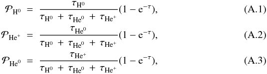 where
τH0,
τHe0 and
τH+ are the optical depths for H0,
He0 and He+ in a given cell, and
τ ≡ τH0 + τHe0 + τH+.
Therefore, the total absorption probability,
where
τH0,
τHe0 and
τH+ are the optical depths for H0,
He0 and He+ in a given cell, and
τ ≡ τH0 + τHe0 + τH+.
Therefore, the total absorption probability,  , for a photon packet
arriving in a cell of optical depth τ is given by
, for a photon packet
arriving in a cell of optical depth τ is given by
 (A.4)For each cell, the
optical depth τ is
(A.4)For each cell, the
optical depth τ is
![\appendix \setcounter{section}{1} \begin{eqnarray} \tau &=& \tau_{\rm{H}^0} +\tau_{\rm{He}^0}+\tau_{\rm{He}^+} \nonumber \\ &=&\left[ \sigma_{\rm{H}^0}(\nu)n_{\rm{H}^0} +\sigma_{\rm{He}^0}(\nu)n_{\rm{He}^0}+\sigma_{\rm{He}^+}(\nu)n_{\rm{He}^+}\right]l, \end{eqnarray}](/articles/aa/full_html/2010/15/aa14347-10/aa14347-10-eq210.png) (A.5)where
σA is the photoionization cross-section for absorber
(A.5)where
σA is the photoionization cross-section for absorber
 ,
,
 , is
number density in the cell and l is the path length in a cell. We use
photoionization cross section fits in Verner et al.
(1996).
, is
number density in the cell and l is the path length in a cell. We use
photoionization cross section fits in Verner et al.
(1996).
If Nγ is the number of photons in a photon
packet arriving in a cell, then the number of photons absorbed in a cell,
NA, is:
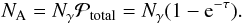 (A.6)The contribution of
photoionization and photoheating to the evolution of the ionization fraction and the
temperature within a time step Δt is:
(A.6)The contribution of
photoionization and photoheating to the evolution of the ionization fraction and the
temperature within a time step Δt is:
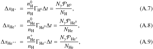
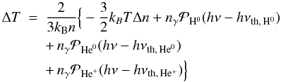 (A.10)where
NH and NHe is the total number
of hydrogen and helium in a cell, hνth,A
are the ionization potential of the recombined atom,
nγ is the
Nγ in a unit volume.
ΓA are the continuous photoionization rates used to
actually integrate the evolution of th ionization fractions. Indeed recombination,
collisional ionization and radiative cooling are treated as continuous process, with
integration time step Δt∗ much less than
Δt using the following coupled equations
(A.10)where
NH and NHe is the total number
of hydrogen and helium in a cell, hνth,A
are the ionization potential of the recombined atom,
nγ is the
Nγ in a unit volume.
ΓA are the continuous photoionization rates used to
actually integrate the evolution of th ionization fractions. Indeed recombination,
collisional ionization and radiative cooling are treated as continuous process, with
integration time step Δt∗ much less than
Δt using the following coupled equations
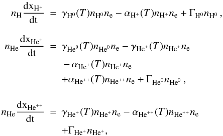 (A.11)where
αI and γA indicate the
recombination and collisional ionization coefficients and
I ∈ {H+,He+,He++}. We use
the values in Hui & Gnedin (1997) for the
recombination coefficient and recombination cooling. For collisional ionization
coefficients and other radiative cooling we use the values in Cen (1992).
(A.11)where
αI and γA indicate the
recombination and collisional ionization coefficients and
I ∈ {H+,He+,He++}. We use
the values in Hui & Gnedin (1997) for the
recombination coefficient and recombination cooling. For collisional ionization
coefficients and other radiative cooling we use the values in Cen (1992).
The temperature is computed from the energy conservation equation. E
is the internal energy of the gas,  .
.
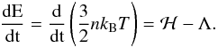 (A.12)ℋ and Λ are the
heating and cooling function which account for the energy gained and lost in a unit
volume per unit time.
(A.12)ℋ and Λ are the
heating and cooling function which account for the energy gained and lost in a unit
volume per unit time.
Each photon packet keeps propagating until it exits the simulation box (if we use free
boundary condition) or until the remaining photon content is much less than the initial
photon content,  .
We typically adopt p = 4 for the UV continuum.
.
We typically adopt p = 4 for the UV continuum.
Appendix B: Validation tests
B.1. Radiative transfer comparison test
A cosmological radiative transfer code comparison project was performed in Iliev et al. (2006a) trying to understand which algorithms (including various flavors of ray-tracing and moment schemes) are suitable for a given non-trivial problem as well as to validate each code by comparing the results with other codes. Five tests are run for radiative transfer in a static density field. We reproduced several of tests in Iliev et al. (2006a) with LICORICE. LICORICE shows good agreements with other codes: results and comparisons with other codes are shown in Baek (2009).
Three additional tests are presented in Iliev et al. (2009) for the coupled gas dynamical and radiative transfer evolution. LICORICE directly participated in this second project and shows good agreements with the other codes.
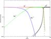 |
Fig. B.1 Comparison of different ionization fractions between LICORICE (circles) and CLOUDY (solid lines), as a function of distance from the point source in cell units (1 pc). |
B.2. Comparison with CLOUDY I: helium
An analytic solution to the radiative transfer evolution of an homogeneous medium around a single source exists only in the isothermal case with only hydrogen. In order to validate helium ionization and spectrum hardening, we reproduced the Strömgren sphere test in Maselli et al. (2003), and compared our results with the 1-D radiative transfer code CLOUDY8 (C08 version of the code).
A point source, emitting as a black body at T = 60000 K with ionizing
luminosity L = 1038ergs-1, is located at the
center of the simulation box in a homogeneous density field with
n = 1 cm-3 composed of hydrogen (90% by number) and
helium (10% by number). The gas is initially completely neutral at a temperature of
T = 102 K in the entire simulation box cube of
Lbox = 128 pc. The comparison is performed at a time
ts = 6 × 10⁵ yr  (where
 is the characteristic time
scale for hydrogen recombination).
is the characteristic time
scale for hydrogen recombination).
The script used for CLOUDY is the following:
blackbody, T=60,000K
luminosity 38
radius 0.01 60 linear parsecs
hden -0.0457
abundances all -15
sphere static
element abundance helium -0.9542
punch element hydrogen "hydrogen_caseA.dat"
punch element helium "helium_caseA.dat"
punch temperature "temperature_caseA.dat"
punch continuum units eV "spectrum_60pc.dat"
In Figs. B.1 and B.2, the comparison between CLOUDY (solid lines) and LICORICE (circles) is shown. The value of the different physical quantities is plotted as a function of the distance from the source, expressed in cell units, Δx = 1 pc. The points represent spherically averaged LICORICE outputs. LICORICE shows a good agreement with CLOUDY. The positions of various ionizing fronts agree within 1%. To obtain this good agreement we consider the effect of secondary ionization and heating by fast electrons as CLOUDY does. The secondary ionization and heating fits in Shull & van Steenberg (1985) are only accurate for the primary photoelectrons higher than 100 eV, so we follow fits in Furlanetto & Johnson Stoever (2010) which is valid for ones less than 100 eV.
The temperature profile shows also a good agreement, except for the warm tail extending beyond the ionizing front for CLOUDY. This warm tail may originate from heat conduction which LICORICE does not implement.
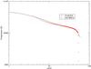 |
Fig. B.2 Comparison of temperature distribution between LICORICE (circles) and CLOUDY (solid lines), as a function of distance from the point source in cell units (1 pc). |
Treating properly the spectrum hardening is an important issue in the radiative transfer with helium. Since each absorber (H0, He0 and He+) has a different ionizing potential, the emitted spectrum will be strongly depleted just above the different ionizing frequencies once it hits a sufficient amount of absorbers. We plot in Fig. B.3 the luminosity per unit surface at different distances and compare between CLOUDY (solid lines) and LICORICE (circles). Our results agree well with the ones of CLOUDY. The noise at higher frequencies (>5 Ryd) is due to the nature of the Monte Carlo method: the tails of the distributions are poorly sampled. At 4 pc, all species are already ionized so the medium is transparent and the spectrum is close to the initial one. At 14 pc, only photons with energy higher than 4 Ryd are absorbed to double ionize He. Above 40 pc, we can observe also the depletion at ~1.8 Ryd, which corresponds to the single ionization of helium.
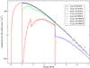 |
Fig. B.3 The luminosity per unit surface at different distances. Comparison between CLOUDY (solid lines) and LICORICE (circles). |
B.3. Comparison with CLOUDY II: X-ray
We have also performed a comparison test with CLOUDY to validate X-ray radiative transfer. The geometrical initial set up is the same as in the test above. Now a point source in the center emits X-ray photons with energy from 100 eV to 2 keV, and a power-law spectrum with α = −1.6 in Eq. (5). The total luminosity is the same as in the helium test, L = 1038ergs-1. The gas is composed of pure hydrogen, and completely neutral at the beginning. The recombination time is proportional to the inverse of electron density. But instead of a sharp ionization front we have a gradual decrease in the ionization fraction with increasing radius. At the boundary of the box, the equilibrium ionization fraction is only ~5% so the recombination time is ~20 times large than in the inner region. Consequently the integration with LICORICE was extended to t = 2500 Myr.
The script used for CLOUDY is the following:
interpolate (1. -10.) (7.34 -10.) (7.35 0.) (147.35 -2.08) (147.4 -10.) (200. -10.)
luminosity 38
radius 0.1 100 linear parsecs
hden -0.0457
abundances all -15
sphere static
punch element hydrogen "hydrogen_Xray.dat"
punch temperature "temperature_Xray.dat"
In Figs. B.4 and B.5, the comparison between CLOUDY (solid lines) and LICORICE (circles) is shown. The value of the different physical quantities is plotted as a function of the distance from the source, expressed in cell units, Δx = 1 pc. The points represent spherically averaged LICORICE outputs. LICORICE shows a very good agreement with CLOUDY. The (very) small difference in the ionization fraction at large radii is due to the fact that we stopped the integration at t = 2500 Myr, which is not much more than one local recombination time: the equilibrium is not fully established. We could integrate for a longer time, but then the problem would only be shifted to larger radii and smaller ionization fractions.
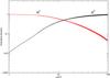 |
Fig. B.4 Comparison of different ionization fractions between LICORICE (circles) and CLOUDY (solid lines), as a function of distance from the point source in cell units (1 pc). |
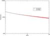 |
Fig. B.5 Comparison of temperature distribution between LICORICE (circles) and CLOUDY (solid lines), as a function of distance from the point source in cell units (1 pc). |
Appendix C: Luminosity, SED, and typical life time of the sources
Let us consider a source particle containing a population of stars. The number of stars dN in a mass interval dM is described by the IMF function ξ(M):
 The properties of a star
of mass M are described by the bolometric luminosity
L(M), the effective blackbody temperature
Teff(M), and its life time
tlife(M). We can write the emissivity of a
single star ϵν
(erg s-1 Hz-1):
The properties of a star
of mass M are described by the bolometric luminosity
L(M), the effective blackbody temperature
Teff(M), and its life time
tlife(M). We can write the emissivity of a
single star ϵν
(erg s-1 Hz-1):
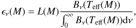 where
Bν is the Planck law. Then we can write
the time dependent emissivity of the complete population
ϵtot as:
where
Bν is the Planck law. Then we can write
the time dependent emissivity of the complete population
ϵtot as:
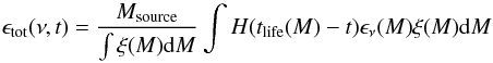 were
H is the Heavy side step function and the integrals over the masses are
bounded by the mass interval in which we want to apply the IMF. With this quantity, we
define a characteristic life-time in a spectral band
[ν1,ν2] :
were
H is the Heavy side step function and the integrals over the masses are
bounded by the mass interval in which we want to apply the IMF. With this quantity, we
define a characteristic life-time in a spectral band
[ν1,ν2] :
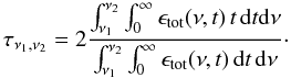 If the total emissivity
was a simple decaying exponential, this definition would give two characteristic decay
times. We choose it as a typical time during which most of the energy has been emitted.
From this we can define the typical constant luminosity emitted in the band as:
If the total emissivity
was a simple decaying exponential, this definition would give two characteristic decay
times. We choose it as a typical time during which most of the energy has been emitted.
From this we can define the typical constant luminosity emitted in the band as:
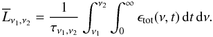 The value of
τν1,ν2
and
The value of
τν1,ν2
and  are
computed in Table 3 for different IMF in the Lyman and ionizing bands. Finally, we can
compute the time-averaged total emissivity:
are
computed in Table 3 for different IMF in the Lyman and ionizing bands. Finally, we can
compute the time-averaged total emissivity:
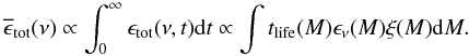 This gives the
constant SED to use during a characteristic life-time, and the normalization is given by
the relation:
This gives the
constant SED to use during a characteristic life-time, and the normalization is given by
the relation:
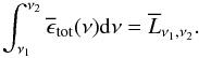
All Tables
Physical properties of low metalicity (Z = 0.004 Z⊙) main sequence stars (Meynet & Maeder 2005).
Averaged luminosities and life times of our source model for a baryon particle depending on the energy band.
All Figures
|
Fig. 1 Normalized spectral intensity of our source model. Black solid line is the SED from Salpeter IMF and red dashed line is from top-heavy IMF. |
| In the text | |
|
Fig. 2 Mass (thicker lines) and volume (thinner lines) weighted ionization fraction of hydrogen. S1 and S3 use Salpeter IMF and S2 use top-heavy IMF. S3 contains helium element. |
| In the text | |
|
Fig. 3 The evolution of the gas temperature of the neutral IGM with redshift. The neutral gas is chosen so that its ionization fraction is less than 0.01. |
| In the text | |
|
Fig. 4 Differential brightness temperature maps for different simulations. The thickness of the slice is ≈ 2 Mpc. The maps in the left column are when ⟨ xα ⟩ = 1, the middles when ⟨ xα ⟩ = 10 and the right when ⟨ xHII ⟩ = 0.5. The black contour separates absorption and emission region. (l) shows no absorption region. |
| In the text | |
|
Fig. 5 Power spectrum evolution of the δTb from the S1 (thin black), S2 (thick black), S6 (thin gray) and S7 (thick gray) simulations. S2 use top-heavy IMF whereas the others use Salpeter IMF. S6 has 1% and S7 has 10% of total luminosity for X-rays. |
| In the text | |
|
Fig. 6 Evolution of the brightness temperature power spectrum with redshift. k = 0.07 h/Mpc (thin black), k = 0.19 h/Mpc (thick black ), k = 1.00 h/Mpc (thin gray) and k = 3.15 h/Mpc (thick gray). |
| In the text | |
|
Fig. 7 The evolution of the 21-cm PDF. The redshifts are 14.05, 10.64 and 8.48 for a), b), and c). The PDFs of panel d) is chosen so that the ionization fraction is 0.5. The red curves on b) are gaussian fits with the mean and variance of the PDFs. |
| In the text | |
|
Fig. 8 Evolution of the skewness with the ionization fraction. |
| In the text | |
|
Fig. B.1 Comparison of different ionization fractions between LICORICE (circles) and CLOUDY (solid lines), as a function of distance from the point source in cell units (1 pc). |
| In the text | |
|
Fig. B.2 Comparison of temperature distribution between LICORICE (circles) and CLOUDY (solid lines), as a function of distance from the point source in cell units (1 pc). |
| In the text | |
|
Fig. B.3 The luminosity per unit surface at different distances. Comparison between CLOUDY (solid lines) and LICORICE (circles). |
| In the text | |
|
Fig. B.4 Comparison of different ionization fractions between LICORICE (circles) and CLOUDY (solid lines), as a function of distance from the point source in cell units (1 pc). |
| In the text | |
|
Fig. B.5 Comparison of temperature distribution between LICORICE (circles) and CLOUDY (solid lines), as a function of distance from the point source in cell units (1 pc). |
| In the text | |
Current usage metrics show cumulative count of Article Views (full-text article views including HTML views, PDF and ePub downloads, according to the available data) and Abstracts Views on Vision4Press platform.
Data correspond to usage on the plateform after 2015. The current usage metrics is available 48-96 hours after online publication and is updated daily on week days.
Initial download of the metrics may take a while.