| Issue |
A&A
Volume 522, November 2010
|
|
|---|---|---|
| Article Number | A112 | |
| Number of page(s) | 15 | |
| Section | Galactic structure, stellar clusters and populations | |
| DOI | https://doi.org/10.1051/0004-6361/200913234 | |
| Published online | 09 November 2010 | |
The ultracool-field dwarf luminosity-function and space density from the Canada-France Brown Dwarf Survey⋆,⋆⋆
1
Observatoire de Besançon, Université de Franche-Comté, Institut Utinam, UMR
CNRS 6213
, BP 1615,
25010
Besançon Cedex,
France
e-mail: celine@obs-besancon.fr
2
School of Physics and Astronomy, University of St Andrews,
North Haugh,
St Andrews
KY16 9SS,
UK
3
Herzberg Institute of Astrophysics, National Research Council, 5071 West Saanich Rd, Victoria, BC
V9E 2E7,
Canada
4 Canada-France-Hawaii Telescope Corporation, 65-1238 Mamalahoa
Highway, Kamuela, HI96743, USA
5
Laboratoire d’Astrophysique de Grenoble, Université J. Fourier,
CNRS, UMR5571, Grenoble, France
6
Département de physique and Observatoire du Mont Mégantic,
Université de Montréal, C.P.
6128, Succursale Centre-Ville,
Montréal, QC
H3C 3J7,
Canada
7
McDonald Observatory, University of Texas at Austin, 1 University
Station C1402, Austin, TX
78712-0259,
USA
Received:
3
September
2009
Accepted:
7
August
2010
Context. Thanks to recent and ongoing large scale surveys, hundreds of brown dwarfs have been discovered in the last decade. The Canada-France Brown Dwarf Survey is a wide-field survey for cool brown dwarfs conducted with the MegaCam camera on the Canada-France-Hawaii Telescope.
Aims. Our objectives are to find ultracool brown dwarfs and to constrain the field brown-dwarf luminosity function and the mass function from a large and homogeneous sample of L and T dwarfs.
Methods. We identify candidates in CFHT/MegaCam i′ and z′ images and follow them up with pointed near infrared (NIR) imaging on several telescopes. Halfway through our survey we found ~ 50 T dwarfs and ~ 170 L or ultra cool M dwarfs drawn from a larger sample of 1400 candidates with typical ultracool dwarfs i′ − z′ colours, found in 780 square degrees.
Results. We have currently completed the NIR follow-up on a large part of the survey for all candidates from mid-L dwarfs down to the latest T dwarfs known with utracool dwarfs’ colours. This allows us to draw on a complete and well defined sample of 102 ultracool dwarfs to investigate the luminosity function and space density of field dwarfs.
Conclusions. We found the density of late L5 to T0 dwarfs to be
 objects
pc-3, the density of T0.5 to T5.5 dwarfs to be
objects
pc-3, the density of T0.5 to T5.5 dwarfs to be  objects
pc-3, and the density of T6 to T8 dwarfs to be
objects
pc-3, and the density of T6 to T8 dwarfs to be  objects
pc-3. We found that these results agree better with a flat substellar mass
function. Three latest dwarfs at the boundary between T and Y dwarfs give the high density
objects
pc-3. We found that these results agree better with a flat substellar mass
function. Three latest dwarfs at the boundary between T and Y dwarfs give the high density
 objects pc-3.
Although the uncertainties are very large this suggests that many brown dwarfs should be
found in this late spectral type range, as expected from the cooling of brown dwarfs,
whatever their mass, down to very low temperature.
objects pc-3.
Although the uncertainties are very large this suggests that many brown dwarfs should be
found in this late spectral type range, as expected from the cooling of brown dwarfs,
whatever their mass, down to very low temperature.
Key words: stars: low-mass / brown dwarfs / stars: luminosity function, mass function / Galaxy: stellar content
Based on observations obtained with MegaPrime/MegaCam, a joint project of CFHT and CEA/DAPNIA, at the Canada-France-Hawaii Telescope (CFHT), which is operated by the National Research Council (NRC) of Canada, the Institut National des Sciences de l’Univers of the Centre National de la Recherche Scientifique (CNRS) of France, and the University of Hawaii. This work is based in part on data products produced at TERAPIX and the Canadian Astronomy Data Centre as part of the Canada-France-Hawaii Telescope Legacy Survey, a collaborative project of NRC and CNRS. Based on observations made with the ESO New Technology Telescope at the La Silla Observatory. Based on observations obtained at the Gemini Observatory, which is operated by the Association of Universities for Research in Astronomy, Inc., under a cooperative agreement with the NSF on behalf of the Gemini partnership: the National Science Foundation (United States), the Science and Technology Facilities Council (United Kingdom), the National Research Council (Canada), CONICYT (Chile), the Australian Research Council (Australia), CNPq (Brazil) and CONICET (Argentina). Based on observations with the Kitt Peak National Observatory, National Optical Astronomy Observatory, which is operated by the Association of Universities for Research in Astronomy, Inc. (AURA) under cooperative agreement with the National Science Foundation. Based on observations made with the Nordic Optical Telescope, operated on the island of La Palma jointly by Denmark, Finland, Iceland, Norway, and Sweden, in the Spanish Observatorio del Roque de los Muchachos of the Instituto de Astrofisica de Canarias. Based on observations made at The McDonald Observatory of the University of Texas at Austin.
Tables 3, 5 and 8 are only available in electronic form at http://www.aanda.org
© ESO, 2010
1. Introduction
Brown dwarfs are very low-luminosity objects. Even at their flux maximum in the near and mid-infrared, brown dwarfs are more than ten magnitudes fainter than solar-type stars. That explains the very low number of detected substellar objects compared to that of known stars, although they probably represent a sizeable fraction of the stellar population in our Galaxy.
The first discoveries of brown dwarfs were made by Nakajima et al. (1995) around the nearby star Gliese 229 and by Stauffer et al. (1994) and Rebolo et al. (1995) in the Pleiades. Delfosse et al. (1997); Ruiz et al. (1997) and Kirkpatrick et al. (1997) found the first field brown dwarfs. Since then, several hundreds of field brown dwarfs have been identified, most of them thanks to large-scale optical and near-infrared imaging surveys because they can be identified by their red optical minus near-infrared colours. Most of them have been found in the Two-Micron All-Sky Survey (2MASS, Skrutskie et al. 2006) and in the Sloan Digital Sky Survey (SDSS, York et al. 2000). See Kirkpatrick (2005) for a review on brown dwarf discoveries.
The new generation of large-area surveys uses deeper images. As a consequence, the number of known brown dwarfs increases and new types of rarer and fainter brown dwarfs are detected (Delorme et al. 2008a; Burningham et al. 2008). Such surveys are the UKIRT Infrared Deep Sky Survey (UKIDSS, Lawrence et al. 2007) and the one we undertook, the Canada-France-Brown-Dwarf Survey (CFBDS, Delorme et al. 2008b). The Canada-France-Brown-Dwarf Survey is based on deep multi-colour MegaCam optical imaging obtained at the Canada-France-Hawaii Telescope (CFHT). We expect that complete characterisation of all our candidates will yield about 100 T dwarfs and over 400 L or very late-M dwarfs, which will approximately double the number of known brown dwarfs with a single, well-characterised survey.
With that large number of identified brown dwarfs, it becomes possible to define uniform and well-characterised samples of substellar objects to investigate their mass and luminosity functions. The knowledge of these functions is essential in several studies. In terms of Galactic studies, it gives clues on the baryonic content of the Galaxy and contributes to determine the evolution of the Galaxy mass. In terms of stellar physics studies, it gives constraints on stellar and substellar formation theories.
It has been shown that a single log-normal function could fit the mass function from field stars to brown dwarfs (see Chabrier 2003; see also Luhman et al. 2007). Our Galaxy probably counts several 1010 of brown dwarfs, hundreds of them in the Solar neighbourhood!
To validate these assumptions, which are mainly based on the study of brown dwarfs in stars clusters, it is necessary to first refine the field brown dwarf luminosity-function. An initial estimate of the local space density of late T dwarfs have been made by Burgasser (2002)1, from a sample of 14 T-dwarfs. Allen et al. (2005) used these results combined with data compiled from a volume-limited sample of late M and L dwarfs (Cruz et al. 2003) to compute a luminosity function. Recently, a detailed investigation on a volume-limited sample of field late-M and L dwarfs has been performed by Cruz et al. (2007). A similar empirical investigation of field T-dwarfs have been presented by Metchev et al. (2008). Still the number of objects in their sample is relatively small (46 L-dwarfs and 15 T-dwarfs, respectively) and the field brown dwarf luminosity-function remains poorly constrained. Thus further efforts are needed to measure the space density of brown dwarfs.
At mid-course of the CFBDS survey, we are able to define an homogeneous sample of 102 brown dwarfs redder than i′ − z′ = 2, from the mid-L dwarfs to the far end of the brown dwarfs observed sequence at the T/Y transition, and to derive a luminosity function. These objects are drawn from a 444 square degree area (57% of the total area) where all candidates with i′ − z′ > 2.0 have been followed-up with near-infrared photometry and, for the reddest of them, with spectroscopy. They represent a sub-sample in colour (i′ − z′ < 2.0) and in magnitude (z′ < 22.5) of the hundreds of brown dwarfs found with i′ − z′ > 1.7 on the entire survey. Section 2 briefly describes the CFBDS and the related observations. The construction of a complete and clean sample of L5 and cooler dwarfs is explained in Sect. 3.2. In Sect. 5, we compare our results with prior studies and link them to the mass function of brown dwarfs. Section 4 presents the luminosity function derived from this sample. Conclusions are given in Sect. 6.
2. Observations
The brown dwarf sample is drawn from the CFBDS. The survey is fully described in Delorme et al. (2008b). The CFBDS is a survey in the i′ and z′ filters conducted with MegaCam (Boulade et al. 2003) at the CFHT. It is based on two existing surveys, the CFHT Legacy Survey (CFHTLS2, Cuillandre & Bertin 2006) and the Red-sequence Cluster Survey (RCS-2, Yee et al. 2007), complemented with significant Principal Investigator data at CFHT. The survey is also extremely effective at finding high-redshift quasars. The parallel programme is called the Canada-France High-z Quasar Survey, and results are presented in Willott et al. (2007, 2009).
The i′ and z′ imaging part of the 780 deg2 CFBDS is nearing completion to typical limit of z′ = 22.5, probing the brown dwarf content of the Galaxy as far as 215 pc for the mid-L dwarfs, 180 pc for the early-type T dwarfs and 50 pc for the late-type T dwarfs.
The reddest sources are then followed-up with pointed J-band imaging to distinguish brown dwarfs from other astronomical sources, and spectra are obtained for the latest type dwarfs.
Throughout this paper, we use Vega magnitudes for the J-band and AB magnitudes for the i′ and z′ optical bands.
2.1. Optical imaging
We only briefly describe the processing and photometry of the imaging observations in this paper. A full description can be found in Delorme et al. (2008b).
Pre-processing of the MegaCam images is carried out at CFHT using the ELIXIR pipeline. This removes the instrumental effects from the images. We then run our own algorithms to improve the astrometry and check the photometry. Finally, we stack the images (if there is more than one exposure at a given position) and register the images in the four different filters. Photometry is carried out with an adaptation of SExtractor (Bertin & Arnouts 1996), which uses dual-image multiple point-spread function fitting to optimise the signal-to-noise ratio (S/N) of point sources.
Candidate brown dwarfs and quasars are initially identified on the optical images as objects which have very high i′ − z′ colours. A 10σ detection in z′ is required but no constraint is set on i′: in several cases, the targets are i′-dropouts and only i′ − z′ lower limits can be determined. As shown in Willott et al. (2005), photometric noise causes many M dwarfs with intrinsic colours of 0.5 < i′ − z′ < 1.5 to be scattered into the region of the diagram at i′ − z′ > 1.5 where we would expect to find only L or T dwarfs and quasars. The huge number of these M stars would require a lot of telescope time for complete follow-up. Therefore, we limit our survey to objects observed to be redder than i′ − z′ > 1.7. Changing this criterion reduces the number of M dwarf contaminants by ~ 95%.
Spectral indices for the the unified scheme of Burgasser et al. (2006) and spectrophotometric distances.
2.2. Near-infrared imaging
As shown by Fan et al. (2001), brown dwarfs and quasars (and artefacts) can be separated with NIR J-band imaging. Willott et al. (2005) described in detail the method for identifying high-redshift quasars and brown dwarfs using MegaCam optical plus near-IR imaging. The very red i′ − z′ of high-redshift quasars is caused by deep Lyman-α absorption on a relatively flat intrinsic spectrum, and they appear significantly bluer than brown dwarfs in z′ − J. On the contrary the spectral distribution of brown dwarfs keeps rising into the J band. We therefore carried out NIR imaging at several observatories: La Silla (New Technology Telescope, 3.6 m), McDonald (2.7 m), Kitt Peak (2.1 m), La Palma (Nordic Optical Telescope, 2.5 m). We obtained the J magnitude for all candidates, dwarfs or quasars. For dwarfs, the signal-to-noise ratio is 10 to 50σ.
Besides pinpointing the few high-redshift quasars that contain important clues on the reionization of the Universe (Willott et al. 2005, 2007, 2009), the J-band photometry very effectively rejects any remaining observational artefacts, as well as the more numerous M stars scattered into the brown dwarf/quasar box by large noise excursions.
2.3. Spectroscopy
Follow-up spectroscopy of the T dwarf candidates with the reddest z′ − J colour was then carried out at Gemini. Before the GNIRS incident at Gemini-South on April 2007 (see Gemini Observatory call for proposal archive, semester 2007B3), it was used in its cross-dispersed mode to obtain a 0.9–2.4 micron coverage. Then NIRI at Gemini-North was used in a two-step approach: 1) H-band spectra were obtained to determine spectral types and 2) T6 and cooler objects were targeted for additional coverage in the J band and occasionally in the K band.
To date we obtained spectroscopic follow-up for 40 T-dwarfs. Four more T-dwarf candidates have been followed-up by Knapp et al. (2004); Chiu et al. (2006); Warren et al. (2007). Spectral types range between T0 and the T/Y transition with 6 dwarfs being of type T7 or later. Four of these have already been presented in (Delorme et al. 2008a,b). Spectral indices of the others are given in Table 1 and are fully described in a forthcoming paper (see also Albert et al. 2009). For all of them we use an absolute magnitude versus spectral type relation instead of the absolute magnitude versus colour used for the other objects (see Sect. 4.1).
3. Defining a homogeneous, complete, and clean sample
3.1. Photometric classification
One square-degree MegaCam image contains several hundred thousand objects, of which at most a few are brown dwarfs. We thus need to strike a careful balance between sample completeness and contamination. To tune this compromise we need a precise knowledge of the colours of brown dwarfs for the exact instruments and filters used in our survey.
The spectral energy distribution obtained from several photometric bands is characteristic of the spectrum of one object. In order to get information on the spectral type of the CFBDS candidates based on its photometry, we determined the colours in the photometric system used by CFBDS of brown dwarfs with known spectral type.
We used publicly available spectra from the L and T dwarf data archive4, (Martín et al. 1999; Kirkpatrick et al. 2000; Geballe et al. 2001; Leggett et al. 2002; Burgasser et al. 2003; Knapp et al. 2004; Golimowski et al. 2004; Chiu et al. 2006) of 45 brown dwarfs with spectral types L1 to T8. Spectral types for L and T dwarfs are given according to the infrared classification scheme described in Geballe et al. (2002) and Burgasser et al. (2006), respectively.
Thus synthetic colours in the MegaCam filters are computed in the AB system (Fukugita et al. 1996) using detector quantum efficiency and transmission curves for the atmosphere, telescope, camera optics, and filters. We similarly synthesised J-band photometry for each of the instruments and J filters used in the J-band follow up. These instruments have significantly different response curves, which must be taken into account to obtain homogeneous selection criteria.
Synthetic colours are given in Table 2. Figure 1 displays the resulting colour–colour diagram. The synthetic colours of each brown dwarf are represented by filled squares. The dashed line shows the resulting colour–colour relation. Spectral types are given along this track, indicating the averaged colour of brown dwarfs at a given spectral type.
Synthetic colours computed on publicly available spectra.
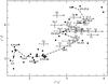 |
Fig. 1 z′ − J synthetic colour versus i′ − z′ synthetic colour computed from available spectra in the literature. i′ and z′ are computed in the CFHT/MegaCam filters, J is computed for the NTT/SOFI Js filter. The filled squares show the colours of each brown dwarf. The dashed line shows the mean colour–colour relation. Spectral types are given along this track, indicating the averaged colour of brown dwarfs with a given spectral type. Crosses with error bars show the T dwarfs for which we obtained spectroscopic observations. An arrow indicates no detection in the i′-band, meaning that the i′ − z′ colour is a lower limit. |
Owing to the high dispersion of brown dwarf colours, the classification of one candidate based on its photometry is not reliable. However, the colours can be used to classify the object within a large category such as early L or late L, the overall classification of the objects being statistically significant. Table 3 gives the locus of the spectral classes in the colour–colour diagram.
In the L-dwarf domain, bright L dwarfs discovered in SDSS or 2MASS and with known spectral type that are also identified on the CFBDS images allow us to validate the colour-based classification. In the T-dwarf domain, we compared the synthetic colours as a function of spectral type with the real colours of T-dwarf candidates that we followed-up spectroscopically. Their locus in the colour–colour diagram is shown by crosses with error bars in Fig. 1. While the agreement is good for early T-dwarfs, it is poor for the late T-dwarfs where the observed z′ − J colours are bluer than the synthetic ones. In particular, some of the coldest known object are located in the same region of the colour–colour diagram as mid-T dwarfs.
Several reasons can be invoked to explain the discrepancy between observed and synthetic colours of late-T. First, the number of available spectra of late T-dwarfs is very small (only five with spectral type later than T6). Because the colour dispersion is quite high for a given spectral type, the mean synthetic colour can be biased by one peculiar object. Next, the synthetic colours of late T-dwarfs may be uncertain, because for these extreme objects with very narrow flux peaks a small error in the optical transmission can lead to large colour uncertainties. However, as we performed spectroscopic follow-up for all candidates with late-T colours, we used their spectral type for classification instead of colours.
3.2. The sample
The CFBDS is composed of several patches – contiguous areas on the sky – with sizes ranging from 9 to 79 deg2. The galactic latitude over a patch is nearly constant, as well as the stellar density and the interstellar reddening. The reddening is low for all patches (~0.011 ± 0.009 for RCS2 patches and ~ 0.020 ± 0.009 for CFHTLS patches). Therefore each patch constitutes a sample of homogenous data.
Because the priority was given for the reddest candidates (i′ − z′ = 2 or redder) for J-band follow-up, we can now build a complete sample of late L and T dwarf candidates over 16 patches with a total effective area of 444 deg2 (Table 4). The sample contains all candidates with z′ < 22.5 and i′ − z′ > 2.0 detected in this area.
Patches used to build a complete sample.
This sample contains 249 objects that are candidates cooler than L5 on the basis of their i′ − z′ colour. However, due to the photometric errors, many contaminants with true colour i′ − z′ < 2.0 enter this sample, such as the more numerous M and early L dwarfs. A classification of the candidates is made on the basis of their position in the i′ − z′/z′ − J diagram, as shown in Fig. 2 and explained in Sect. 3.1 (see Table 3 for a summary). Based upon this classification, 102 of the 249 objects remain L5 and later dwarf candidates (Table 3), the others are dwarfs earlier than M 8, artefacts, or quasars. Dwarfs of spectral type > M8 to L5 are theoritically not retained by the i′ − z′ > 2.0 criteria. But they could statistically contaminate our > L5 sample if their i′ − z′ colour is reddened by photometric errors; then the z′ − J criteria will not reject them because they have similar colours as the > L5 dwarfs in this wavelength bandpass. This contamination has to be carefully estimated (Sect. 3.4). The distribution of objects within the spectral classes is given in Table 6.
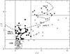 |
Fig. 2 z′ − J versus i′ − z′ diagram of the brown dwarf candidates in our sample with complete J-band follow-up. Open circles: dwarfs earlier than M 8. Filled circles: M 8 to L dwarfs. Open triangles: early T dwarfs. Filled triangles: late T dwarfs. The dotted line shows the colour–colour relation derived in Sect. 3.1. The solid lines show the different spectral type regions defined in Table 3. Note that to build the T dwarfs luminosity-function we did not use this colour-based classification but used the spectral type obtained with spectroscopic follow-up whenever available. |
Preliminary classification of the sample based on the i′ − z′ and z′ − J colours.
3.3. Completeness
Owing to photometric errors, some objects with true colours within our selection criteria are spread out of our selection box and are not identified. Given the depth of CFBDS, one cannot estimate the completeness with a reference sample of objects detected in the images with previously known magnitude and colours. To obtain a reference sample we built a point spread function (PSF) model for each science image using PSfex (E. Bertin, private communication) and created fake stars with 1.2 < i′ − z′ < 4 and 20 < z′ < 23.5 with Skymaker (Bertin 2009). These artificial stars are thus a PSF model scaled to the desired magnitude, affected with a realistic photon noise. This model is oversampled so that it handles correctly the randomised non-integer pixel position of the fake stars. We then added these stars to the science images from which the PSF model was derived, which means that any analysis of these fake stars is affected by the same background noise, bad pixels, saturated stars, and cosmic ray distribution as the actual stars are.
To avoid any significant increase of the image crowding caused by this addition, we injected a number of artificial stars that is lower than 5% of the number of astrophysical sources on the images. This left us with a statistically comfortable sample of 1 500 000 artificial ultracool dwarfs. Drawing upon this sample we were able to derive CFBDS’s completeness.
The resulting images, containing both astrophysical sources and fake stars, went through the same analysis and selection pipelines used to select true candidates. The injection of fake objects in the science images allows us to take into account all effects such as cosmic rays, bad pixels, resampling noise, and possible selection biases when going through the selection pipeline. The effect of faint sources being lost due to the presence of a nearby bright star is also perfectly taken into account without the use of the somewhat arbitrary masking of a given area around saturated stars: their recovery rate directly depends on their magnitude and separation to the saturated stars actually present in the science images. The injection of stars into the actual science images is a direct and extremely robust measure of completeness regardless of what actually causes the loss of completeness.
Thus we can count the number of detected objects as a function of magnitude on the detection image (z′-band) and colour. This is done separately for each patch of the CFBDS. The completeness is given by the fraction of recovered fake objects at the end of the analysis process. Note that the measured colours and magnitudes of fake objects are different from the injected colours because of noise and measurement errors. Figure 3 shows the completeness averaged over the patches of the RCS-2 survey as a function of “true” (that is before going through the analysis process) magnitude and colour. We note cij the completeness in each bin (i,j) of 0.1 mag in magnitude and colour. Note that this completeness does not merely reflect the number of objects detected, but the number of detected objects which went through our whole pipeline and were selected as ultracool dwarfs candidates with a star-like shape, a signal-to-noise ratio over 10, a measured i′ − z′ colour over our selection criterion (i′ − z′ > 2.0 for the sub-sample studied here), and a measured z′ magnitude below 22.5.
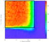 |
Fig. 3 Completeness of the RCS2 component of the CFBDS survey as a function of z′ magnitude and i′ − z′ colour. The colour bar ranges from 0% (blue, all objects went out of the selection limits) to 100% (red, all objects detected). The volume-weighted average completeness over our selection criterion (black rectangle, i′ − z′ > 2.0 and z′ < 22.5) is 73%. This plot also highlights the contamination of our sample by objects whose actual colours and magnitudes lay outside our selection box but are scattered inside by photometric errors. |
Moreover, the measured magnitudes are compared with the “true” ones to derive an error probability distribution (Fig. 4). It gives the probability for one object in a given patch to have a different measured photometry by a given number of σ from its true photometry. The result is very close to a Gaussian distribution, the only difference is found in the wings at more than 5σ, where the number of deviations stands at 1–2%, several orders of magnitude above a Gaussian distribution. This is due to blended objects with galaxies, bad pixels, etc. This distribution, which also takes into account the correlation between pixels caused when resampling any images, will be used when computing the contamination of the sample (Sect. 3.4).
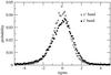 |
Fig. 4 Probability error distribution for one of the RCS2 patches, in the i′ and z′ bands. The errors are given in number of σ. They are computed by comparing the magnitudes of the fake cool dwarfs when injected in the science images with their measured magnitudes. |
3.4. Contaminants
Reddened stars are not possible contaminants because the CFBDS fields are in a low galactic extinction area (i′ − z′ galactic reddening < 0.02 mag). Giant stars are not expected in our sample because with the apparent magnitude of our sample (z′ between 18.5 and 22.5) they would be located at 100 kpc to 1 Mpc, well outside of the Milky Way. Actually, we noticed a contamination by giant stars for fields close to Messier galaxies that we had to eliminate from the survey.
Extremely reddened galaxies could potentially have i′ − z′ and z′ − J colours the same as those of brown dwarfs. These galaxies would have to be at a fairly high redshift (z > 1) for two reasons: (i) higher redshift means shorter rest-frame wavelengths and therefore a lower AV to give the red observed colours; (ii) the CFBDS objects are unresolved in good seeing (typically 0.6 − 0.8′′) and lower redshift galaxies would be easily resolved. However, the high redshift necessary, coupled with the fairly bright J magnitudes of the CFBDS objects and the fact that the red z′ − J indicates significant extinction still at J (e.g. about 3 mag of extinction for rest-frame E(B − V) = 1), means these galaxies would need to have extremely high intrinsic absolute magnitudes and stellar masses ( > 2 × 10¹²M⊙). Galaxies of this mass are extremely rare at redshift z ~ 1 (Drory et al. 2009), and are composed of evolved stellar populations rather than dusty starbursts (Taylor et al. 2009). These massive galaxies would likely be resolved by ground-based seeing out to redshift z ~ 2 (Mancini et al. 2010). In conclusion, we find that high-redshift unresolved galaxies cannot appear as red as the L and T dwarfs and do not cause a significant contaminant.
As already mentioned, high-redshift quasars have the same i′ − z′ colour as brown dwarfs but are easily removed form the sample through their bluer z′ − J colour by about one magnitude. Moreover, they are rare objects, so their contamination is indeed negligible.
As shown in the colour–colour graph in Fig. 1 our sample selects L5 and cooler dwarfs. However, each Megacam field shows on average 50 000 sources, of which about one is selected as a brown dwarf candidate, meaning that non-brown dwarf sources outnumber brown dwarfs by more than a factor 10 000, making 3 or 4σ photometric noise scattering a probable source of contamination, particularly in the i′ band where brown dwarfs are faint and observed at low signal-to-noise ratio and a fraction of earlier type dwarfs with true colour i′ − z′ < 2.0 are sent within the i′ − z′ > 2.0 sample (see Fig. 3). This contamination has to be estimated carefully because earlier dwarfs are much more numerous in a limited-magnitude sample than the later ones.
There is only a small probability for a given object to have large photometric deviations in two independent filters. Therefore the J-band observations at a good S/N ratio are useful to identify a significant fraction of the contaminants. All objects with z′ − J < 2.5 are removed from the sample. This selection rejects (1) artefacts with obviously no J-band detection, (2) quasars, and (3) dwarfs with true i′ − z′ colour lower than 1.3, corresponding to spectral type earlier than M 8, and reddening by photometric noise.
The contamination in z′ − J does exist but has a much lower impact on our study for several reasons: (i) we only obtain J magnitudes for the selected candidates, 249 objects, which make several sigma noise excursions non-significant. This is especially true because the signal-to-noise ratio in J is much better than in i′, leading to much smaller photometric errors, typically in the 0.02–0.1 mag range; (ii) because the colour spectral type relation is very steep at the M 7–M 8.5 transition, going from z′ − J = 2.3 to z′ − J = 2.9, we are confident that possible contamination from earlier than M8 dwarfs part of our 249-strong brown dwarf candidates sample into our z′ − J confirmed brown dwarf sample trough 4 to 8σ noise excursion is marginal; (iii) our sample is z′ selected, so the flux limit bias or Eddington bias that occurs due to a scattering of sources fainter than our z′ magnitude limit into the sample will act to increase the number of high i′ − z′ objects, but decrease the number of high z′ − J′ objects. In practice this bias is very small in both directions because we have a 10 σz′ limit; (iv) the main reason the scattering from low i′ − z′ to high i′ − z′ is so bad is because the number density of objects with true low i′ − z′ is so much higher than those with true high i′ − z′. The opposite is actually true for the L and T dwarfs: in our i′ − z′ selected sample, there are more objects with true high z′ − J (L and T dwarfs) than low z′ − J (z ~ 6 quasars).
The z′ − J cut cannot distinguish ultracool dwarfs with true colour 1.3 < i′ − z′ < 2.0 because they have the same z′ − J colour as late L and early T dwarfs. We therefore need to evaluate the number of potential contaminants that populate this colour range and can leak into our selection through photometric errors. The estimate of the number of contaminants with true colour 1.7 < i′ − z′ < 2.0 is done in two steps as explained below and is done separately for each patch.
-
1.
Six patches of the CFBDS have J-band follow-up for all the candidates with measured colour i′ − z′ > 1.7. These patches contain 228 candidates over a total area of 199 deg2. The z′ − J diagnostic shows that 35% of these objects have indeed spectral type later than M8; the 65% another objects are < M 8, artefacts or quasars. We assume that this value of 35% is representative of the fraction of > M 8 in the 1.7 < i′ − z′ < 2.0 sample for all the patches. These > M 8 dwarfs are the main sources of contaminations in our > L5 stellar count.
-
2.
Thus we compute the probability to get a M 8 to L4.5 dwarf with true colour 1.7 < i′ − z′ < 2.0 but resulting colour i′ − z′ > 2.0. We draw a photometric error in the i′ and z′ bands for 35% of the objects with 1.7 < i′ − z′ < 2.0. Objects with resulting i′ − z′ > 2.0 and z′ < 22.5 are the contaminants. In practical, we added a photometric error to all objects with 1.7 < i′ − z′ < 2.0, and each object that enters our selection box will count for only 0.35 contaminant, which provides a smoother contaminant distribution.
This analysis underestimates the number of contaminants because we do not consider direct contamination from the 1.3 < i′ − z′ < 1.7 colour range to i′ − z′ > 2.0, but also overestimates the number of contaminants because some objects within our 1.7 < ′i − z′ < 2.0 contaminants sample are themselves contaminants with bluer true colours. However these effects to compensate each other: from a statistical analysis of 300 000 fake objects, Delorme (2008)5 derived the contamination percentage from a colour bin to another and showed that the overall probability for any of the objects in the 1.3 < i′ − z′ < 1.7 colour range to be falsely taken into account in our contamination calculation as a potential contaminant is 0.35%.
The number of contaminants in our 444 deg2 sample is obtained in z′ magnitude bins of 0.1 mag and i′ − z′ colour bins of 0.1 mag. The number of objects in these small bins is usually smaller than 1. This number represents the probability of contamination within one bin. The total number of contaminants is 30, among which 23 have a resulting colour i′ − z′ < 2.2.
4. The brown dwarf space-density
The CFBDS patches contain a sufficient number of images and candidates to provide significant statistics. Completeness and contamination are thus handled separately in each patch before combining all data to derive the brown dwarf space-density.
In order to take into account the photometric errors, each object is spread over a colour range following the probability error distribution already used for contaminants (Fig. 4). In this process, we take into account that the true colour of the object is more likely to be bluer than redder, considering the density gradient as a function of i′ − z′ colour: the probability shown in Fig. 4 is weighted by the ratio of densities at the new colour and the observed colour, where densities as a function of colour are derived from our sample. Resulting objects with new i′ − z′ colours and new z′ magnitudes beyond our selection limits are removed. Each object is thus split into several objects (about one hundred) whose weight is smaller than one, representing the actual likelihood that the object belongs to a given colour bin for a given observed colour. The final weight w is obtained by dividing by cij, the completeness in the colour-magnitude bin (i,j). The contaminants are assigned a negative weight.
We determine the luminosity function of ultracool field dwarfs with the generalised form of the Vmax classical technique (Schmidt 1968), which allows to consider density gradients in the Galactic disc. We compute the maximum volume probed by our magnitude-limited survey at a given colour (that is at a given absolute magnitude). This geometric volume is corrected to take into account the decrease of the stellar density with increasing distance above the Galactic plane (Felten 1976; Stobie et al. 1989; Tinney et al. 1993):
![$$V_{\rm Gen}=\Omega\frac{h^3}{\sin^3|b|}[2-(\xi^2+2\xi+2)\exp(-\xi)],$$](/articles/aa/full_html/2010/14/aa13234-09/aa13234-09-eq84.png) where Ω is the area of
the survey, b is the Galactic latitude of the field, h is
the thin disc scale height (h ~ 250 pc from Robin et al. 2003), and
where Ω is the area of
the survey, b is the Galactic latitude of the field, h is
the thin disc scale height (h ~ 250 pc from Robin et al. 2003), and  with d
the maximum distance of detection.
with d
the maximum distance of detection.
For each object d is estimated. Thus the object is counted as the inverse of the maximum volume VGen in which it is observed. The luminosity function is the sum over all objects within an absolute magnitude bin:
 where
w is the weight assigned to each object in this colour bin, taking into
account the photometric errors and the completeness, as explained above.
where
w is the weight assigned to each object in this colour bin, taking into
account the photometric errors and the completeness, as explained above.
The parallax is obtained from absolute magnitude–colour relations as described below.
4.1. Absolute magnitude versus colours and spectral type relations
Among the publicly available spectra found in the L and T dwarf data archive that are used to derive synthetic colours (Sect. 3.1), 32 also have measured parallax. They allow us to derive an absolute magnitude colour relation. The absolute magnitude-colour diagrams are shown in Figs. 5 and 6. The symbols indicate the different spectral classes: open circle for a M 7 dwarf, open squares for M 8 to L4.5 dwarfs, filled circles for L5 to L9.5 dwarfs, open triangles for T0 to T4.5 dwarfs and filled triangles for T5 and later dwarfs. The dotted line shows the derived absolute magnitude–colour relation. The scatter around the relations ranges from 0.2 to 0.8 mag with a mean value of 0.5 mag.
As one can see in the upper panels of Fig. 5, the i′ − z′ colour is a good luminosity estimator for late M and L dwarfs, as shown before in the SDSS photometric system (West et al. 2005). In the T dwarf domain, the i′ − z′ colour is a poor luminosity estimator. Moreover many T dwarfs are not detected in the i′ band. Thus we use the z′ − J colour as a proxy. However the absolute z′ and J band magnitudes of early T dwarfs are nearly constant. This translates into a flux increase in the z′ and J bands from L8 to T4 spectral types (known as J-band bump, Dahn et al. 2002; Tinney & Burgasser 2003; Vrba et al. 2004), contrarily to the classical decrease of luminosity with increasing spectral type. This behaviour at the L-T transition might be caused by the clearing of dust clouds in the atmosphere that reveals a deeper and higher temperature region of the atmosphere (Burgasser et al. 2002; Knapp et al. 2004).
Of our candidates, 32 were found to be T dwarfs from their spectroscopic follow-up. They
are plotted in Fig. 6 (circled symbol) with their
observed z′ − J colour and with
MJ and  determined from brown dwarfs
with known parallax that have the same spectral type. Whereas the agreement is good for
early T dwarfs (open triangles), the synthetic colours of late T dwarfs may be biased and
are redder than the observed colours of T dwarfs with similar spectral type, as already
discussed in Sect. 3.1, We performed spectroscopic
follow-up for all of our candidates with
z′ − J > 4. Thus we do not use their
z′ − J colour to derive their absolute magnitude but
use their spectral type instead. Absolute magnitude versus spectral type relations are
shown in Fig. 7.
determined from brown dwarfs
with known parallax that have the same spectral type. Whereas the agreement is good for
early T dwarfs (open triangles), the synthetic colours of late T dwarfs may be biased and
are redder than the observed colours of T dwarfs with similar spectral type, as already
discussed in Sect. 3.1, We performed spectroscopic
follow-up for all of our candidates with
z′ − J > 4. Thus we do not use their
z′ − J colour to derive their absolute magnitude but
use their spectral type instead. Absolute magnitude versus spectral type relations are
shown in Fig. 7.
To summarise, we use – Mz′ and MJ vs. i′ − z′ relations for i′ − z′ < 2.4 (L dwarfs):
 –
Mz′ and
MJ vs.
z′ − J relations for
i′ − z′ > 2.4 (early-T dwarfs):
–
Mz′ and
MJ vs.
z′ − J relations for
i′ − z′ > 2.4 (early-T dwarfs):
 –
Mz′ and
MJ vs spectral type relations for dwarfs
with spectroscopic follow-up (part of the early-T dwarfs and all late-T dwarfs).
–
Mz′ and
MJ vs spectral type relations for dwarfs
with spectroscopic follow-up (part of the early-T dwarfs and all late-T dwarfs).


 |
Fig. 5
MJ and |
 |
Fig. 6 Same as Fig. 5 for the z′ − J colour. Additional objects are shown (circled symbols). They are our candidates with spectroscopic follow-up. For these objects, z′ − J is the observed colour and the absolute magnitude is derived from their spectral type. The dotted line shows the derived absolute magnitude-colour relation valid for the early-T dwarfs. Error bars are indicated when larger than the symbol. Note that only objects with measured parallax – non circled objects – are used to derive the relation. |
 |
Fig. 7 MJ and |
4.2. Photometric distances
The previous relations are used to derive the photometric distances of the brown dwarfs in our sample. The scatter in the absolute magnitude-colour relation translates to an uncertainty of 26% on the distance estimate. Figure 8 shows the distribution of photometric distances obtained from the z′ magnitudes without (solid line) and with (dotted line) contamination and completeness correction of the sample. It mostly contains brown dwarfs within 20 pc and 120 pc, which most probably belongs to the galactic disc, although it may contain close subdwarfs that can be revealed by high kinematics or low-metallicity features in the spectrum (Burgasser et al. 2002; Geballe et al. 2002; Burgasser et al. 2009; Burningham et al. 2010a). The distribution peaks between 60 and 100 pc, which is about the maximal detection distance for late-L and mid-T dwarfs. Most of the objects detected farther away than 120 pc are early T dwarfs brighter than both late L and mid-T because of the J and z′-bump.
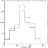 |
Fig. 8 Photometric distance distribution computed in the z′ band of our sample, without (solid line) and with (dotted line) contamination and completeness correction. |
4.3. Malmquist bias
The Malmquist bias (Malmquist 1920) comes from the intrinsic dispersion in the absolute magnitude-colour relations and the limited-magnitude definition of the sample. A given colour (or spectral type) does not correspond to a unique luminosity, but rather a distribution due to intrinsic scatter in metallicity and age, and non detected binaries that appear brighter for their colour. This dispersion has two distinct effects:
-
for a limited-magnitude sample, the mean absolute magnitudeobserved
 is lower than the true mean magnitude
 of objects with a given colour: among the most distant objects, the intrinsically
most luminous ones are detected only (where the true intrinsic absolute magnitude
M0 > M);
of objects with a given colour: among the most distant objects, the intrinsically
most luminous ones are detected only (where the true intrinsic absolute magnitude
M0 > M); -
the number of stars with given apparent magnitude and colour is larger, the brightest stars being observed at larger distances d and the number of objects increasing as d3.
Malmquist (1920) gave the first correction method for this bias, assuming a Gaussian distribution of the luminosity at a given colour, and later Stobie et al. (1989) proposed the following analytic correction:
 where
σ is the luminosity dispersion, Φ the luminosity function, and
where
σ is the luminosity dispersion, Φ the luminosity function, and
 . The first
term is the volume element correction, the second term corrects for the magnitude
translation from M to M0.
. The first
term is the volume element correction, the second term corrects for the magnitude
translation from M to M0.
Because we already took into account the uncertainties in the colours due to photometric errors, σ only depends on the scatter in the absolute magnitude-colour relation. This scatter ranges from 0.2 to 0.8 mag. We consider the mean value σ = 0.5 mag.
4.4. The luminosity function of systems
Our magnitude-limited sample is also biased by binarity effect. An object in a
non-resolved binary system appears brighter and enters our sample contrarily to the same
isolated object. This also affects the colour of the objects. Direct imaging surveys
(Gizis et al. 2003; Bouy et al. 2003) that probe separations of > 2 AU show that
~10 − 15% of field brown dwarfs are binaries with separations that peak between
2 and 4 AU. Lower separations probed by spectroscopic surveys (see Joergens 2008, and references therein) contribute a further
 % (separations
< 0.3 AU) or
% (separations
< 0.3 AU) or  % (separations
< 3 AU). The true BD binary fraction is likely between 15 and 25%, similar to
estimates from Basri & Reiners (2006).
% (separations
< 3 AU). The true BD binary fraction is likely between 15 and 25%, similar to
estimates from Basri & Reiners (2006).
The purely observational data are not the luminosity function but a stellar count as a function of colour and magnitude. To obtain the luminosity function of the systems a first transformation is done with colour-magnitude or spectral type-magnitude relations. Bias could be introduced during this first step, but the relations used (and their limitations) are relatively well known. So the luminosity function of the systems is a good proxy to compare stellar counts of different surveys (with different sets of filters and magnitude limits). Moreover, it is the luminosity function of systems which is used for estimating the number of sources in any survey (with different seeing and spatial resolution).
As explained above, the correction of this function in a true luminosity function (density of stars by magnitude bin) requires the knowledge of the statistical multiplicity (fraction of binaries, triple and higher order systems unresolved and distribution of mass ratios between the components). To date such statistics for brown dwarfs have still a significant margin of error. Hence in this paper we chose to present the luminosity function of systems defined as the luminosity function uncorrected from the bias due to multiple stars.
Figure 9 shows the luminosity function of systems in the z′ and J bands obtained from the brown dwarf sample corrected from contamination and completeness. The number of objects in magnitude bins are also indicated. The values are listed in Table 7. Error bars represent the 95% confidence level interval, derived from Bayesian statistics assuming a Poissonian distribution and a conjugate prior following the method described by Metchev et al. (2008).
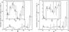 |
Fig. 9 Luminosity function of systems computed in the z′ band (left) and the J band (right) of our sample. |
Brown dwarfs J-band and z′-band luminosity function Φ (10-3 objects pc-3 mag-1).
One notices an increase at the faintest absolute magnitudes, due to T8 and later dwarfs. However, the uncertainties are very large, based on three objects only and the luminosity function remains consistently flat. Furthermore, the luminosity-spectral type relation used for distance estimate is rather rough (see Fig. 7). Assuming a luminosity 0.5 mag brighter leads to a luminosity function twice smaller in these bins. However, the T8.5 dwarf found around a M 4 dwarf with measured parallax (Burningham et al. 2009,open square in Fig. 7) tends to show that the late-T dwarfs luminosity is not underestimated, on the contrary. This uptick in number count is expected from luminosity function simulations (see Allen et al. 2005, and the pile-up of objects with Teff < 500 K in their Fig. 2).
Finding half of the known ultracool brown dwarfs ( > T8) could have been a statistical fluke. Future ultracool brown dwarf discoveries will build up this statistic and check whether this significant increase at the lower end of the luminosity function that we find here is real or not. If true, this would mean either that the lowest mass brown dwarfs are more numerous than expected – which would be different to what is observed in young cluster (see e.g. Moraux et al. 2007) – or that the number of old brown dwarfs of any mass is high. Indeed, whatever their mass, brown dwarfs cool down to the latest and coldest end of the spectral range after a few Gyr and should accumulate there because the cooling rate significantly slows down at these low temperatures. This speculation would agree interestingly with the hints from Gould et al. (2009) that old-population brown dwarfs could be much more numerous than young ones, based on their a priori low probability detection of a thick-disk brown dwarf in a microlensing event.
5. Discussion
Table 8 summarises the comparison with other brown dwarf space densities in MJ bins: the space density from Cruz et al. (2007) computed from a 20 pc volume-limited sample of M 7 to L8 dwarfs and the one obtained Allen et al. (2005) from a sample of 14 T-dwarfs and a volume-limited sample of late M and L dwarfs. As seen in Fig. 1, the T dwarfs can be selected from their i′ − z′ colours larger than 2.6. For objects with no i′ detection, the z′ − J > 3.5 limit is also a good selection criterion for T dwarfs. Thus it is possible to compute the space density for T-dwarfs in different spectral type ranges and to compare with Metchev et al. (2008) result . Our results agree with others. For early-T-dwarfs, they agree with the lower value found by Metchev et al. (2008).
The most important aim in deriving the luminosity function for ultracool dwarfs is setting constraints on the mass function. The computation of mass function from the luminosity function is quite straightforward for stars whose luminosity follows a simple function of their mass. The case is more complex for brown dwarfs that undergo continuous cooling and gravitational contraction during their life. The decrease of luminosity with time provokes a degeneracy: a low-mass brown dwarf can be as bright as a higher mass brown dwarf if younger. The only way to determine age and mass is to compare the spectra with theoretical atmosphere models, which still give quite uncertain results, because the physics of these cool atmospheres is very complex and not yet totally understood. The non-relation between mass and luminosity makes difficult the determination of the mass function. A detailed determination of the substellar mass function is beyond the scop of this paper.
Comparison of the brown dwarf space densities ρ (10-3 objects pc-3) obtained by Burgasser (2007) from simulations assuming different mass functions: Ψ(M) = dN / dM ∝ M − α.
However, first estimates of the substellar mass function have been obtained in the L-dwarf domain: Reid et al. (1999) with 1 < α < 2, Burgasser (2002) 0.5 < α < 1, Allen et al. (2005)α < 0.3 ± 0.6, where α is the slope of the power-law mass function Ψ(M) = dN / dM ∝ M − α. These results are consistent with the substellar mass function in young open clusters showing α ≃ 0.6 (e.g. Caballero et al. 2007; Moraux et al. 2007; Luhman 2007). Recently, Metchev et al. (2008) derived a T dwarf space density that was mostly consistent with α = 0 and the comparison of the observed number of T4-T8.5 dwarfs by Pinfield et al. (2008) favoured α < 0. The analysis of 47 T-dwarfs found in the Large Area Survey (LAS) of UKIDSS also suggests that the substellar mass function is declining at lower masses (Burningham et al. 2010b).
Burgasser (2007) performed simulations assuming different mass functions. The comparison between our luminosity function and these simulations is shown in Table 9. It suggests that the best agreement is obtained with a flat mass function (α = 0) or even a decreasing mass function. Note that our values disagree for early T-dwarfs. However, the physics at the L/T transition is difficult to model, not only due to the cooling of the atmosphere but also to the clearing of the atmosphere that needs to model properly the hydrodynamics and the clouds formation (Freytag et al. 2010), making the timescales uncertain. If confirmed, this low value would back Burgasser et al. (2007) suggestion that the L/T transition occurs rapidly.
Pinfield et al. (2008) suggested that a single power-law exponent is not optimal when describing the substellar mass function in the field, or that the different measured α values result from different models used to convert between mass and magnitude. Further studies based on more extended samples, such as the one we will be able to define at the completion of the CFBDS survey, or from the ongoing Large Area Survey performed by UKIRT, are needed to make reliable investigations on the mass function of field brown dwarfs.
6. Conclusions
At mid-course of the CFBDS, we define a uniform sample to investigate the field brown dwarf
luminosity-function. We obtained spectroscopic follow-up for most of T-dwarf candidates.
Because it is not realistic to obtain spectra for all L-dwarf candidates, we used the noise
properties of the images to compute the contamination and completeness with good enough
accuracy to properly characterise the sample. The sample covers a large spectral type range,
including the L-T transition. It contains 56 L-dwarfs cooler than L5 and 41 dwarfs along the
whole T-dwarfs sequence. We have measured the density of late L5 to T0 dwarfs to be
objects
pc-3, the density of T0.5 to T5.5 dwarfs to be objects
pc-3, and the density of T6 to T8 dwarfs to be objects
pc-3. Three latest dwarfs at the boundary between T and Y dwarfs give the high
density objects
pc-3, although the uncertainties are very large and the luminosity function is
still consistent with being flat. Since then, at least three ultracool brown dwarfs
(> T8) have also been discovered in UKIDSS (Burningham et al. 2008, 2009) that
currently probes a slightly higher but comparable volume for late-T dwarfs. Even if these
combined statistics still deal with a low number of objects, this could indicate that the
number of ultracool brown dwarfs found by the CFBDS is not entirely due to a fluke of
statistics and that many of these objects remain to be discovered in the solar
neighbourhood. This can be expected as, whatever their mass, brown dwarfs cool down and
finally accumulate in this spectral type range.
Online material
Definition of spectral classes from the i′ − z′ and z′ − J colours.
Photometry of L5 and later dwarf candidates in the MegaCam photometric system.
Comparison of the brown dwarf space densities ρ (10-3 objects pc-3) obtained from CFBDS given separately for L and T-dwarfs, and Allen et al. (2005); Cruz et al. (2007); Metchev et al. (2008).
Acknowledgments
Financial support from the “Programme National de Physique Stellaire” (PNPS) of CNRS/INSU, France, is gratefully acknowledged. We thank the queue observers at CFHT who obtained data for this study. We also thanks the NTT and NOT support astronomers for their help during the observations which led to these results. This research has made use of Aladin, operated at CDS, Strasbourg.
References
- Albert, L., Artigau, É., Delorme, P., et al. 2009, in AIP Conf. Ser., ed. E. Stempels, 1094, 485 [Google Scholar]
- Allen, P. R., Koerner, D. W., Reid, I. N., & Trilling, D. E. 2005, ApJ, 625, 385 [NASA ADS] [CrossRef] [Google Scholar]
- Basri, G., & Reiners, A. 2006, AJ, 132, 663 [Google Scholar]
- Bertin, E. 2009, Mem. Soc. Astron. Ital., 80, 422 [Google Scholar]
- Bertin, E., & Arnouts, S. 1996, A&AS, 117, 393 [NASA ADS] [CrossRef] [EDP Sciences] [Google Scholar]
- Boulade, O., Charlot, X., Abbon, P., et al. 2003, in Instrument Design and Performance for Optical/Infrared Ground-based Telescopes, Presented at the Society of Photo-Optical Instrumentation Engineers (SPIE) Conference, ed. M. Iye, & A. F. M. Moorwood, Proc. SPIE, 4841, 72 [Google Scholar]
- Bouy, H., Brandner, W., Martín, E. L., et al. 2003, AJ, 126, 1526 [NASA ADS] [CrossRef] [Google Scholar]
- Burgasser, A. J. 2002, Ph.D. Thesis, California Institute of Technology [Google Scholar]
- Burgasser, A. J. 2007, ApJ, 659, 655 [NASA ADS] [CrossRef] [Google Scholar]
- Burgasser, A. J., Kirkpatrick, J. D., Brown, M. E., et al. 2002, ApJ, 564, 421 [NASA ADS] [CrossRef] [Google Scholar]
- Burgasser, A. J., Kirkpatrick, J. D., Burrows, A., et al. 2003, ApJ, 592, 1186 [NASA ADS] [CrossRef] [Google Scholar]
- Burgasser, A. J., Geballe, T. R., Leggett, S. K., Kirkpatrick, J. D., & Golimowski, D. A. 2006, ApJ, 637, 1067 [NASA ADS] [CrossRef] [Google Scholar]
- Burgasser, A. J., Cruz, K. L., & Kirkpatrick, J. D. 2007, ApJ, 657, 494 [NASA ADS] [CrossRef] [Google Scholar]
- Burgasser, A. J., Lépine, S., Lodieu, N., et al. 2009, in AIP Conf. Ser., ed. E. Stempels, 1094, 242 [Google Scholar]
- Burningham, B., Pinfield, D. J., Leggett, S. K., et al. 2008, MNRAS, 391, 320 [NASA ADS] [CrossRef] [Google Scholar]
- Burningham, B., Pinfield, D. J., Leggett, S. K., et al. 2009, MNRAS, 395, 1237 [NASA ADS] [CrossRef] [Google Scholar]
- Burningham, B., Leggett, S. K., Lucas, P. W., et al. 2010a, MNRAS, 404, 1952 [NASA ADS] [Google Scholar]
- Burningham, B., Pinfield, D. J., Lucas, P. W., et al. 2010b, MNRAS [Google Scholar]
- Caballero, J. A., Béjar, V. J. S., Rebolo, R., et al. 2007, A&A, 470, 903 [NASA ADS] [CrossRef] [EDP Sciences] [Google Scholar]
- Chabrier, G. 2003, PASP, 115, 763 [NASA ADS] [CrossRef] [Google Scholar]
- Chiu, K., Fan, X., Leggett, S. K., et al. 2006, AJ, 131, 2722 [NASA ADS] [CrossRef] [Google Scholar]
- Cruz, K. L., Reid, I. N., Liebert, J., Kirkpatrick, J. D., & Lowrance, P. J. 2003, AJ, 126, 2421 [NASA ADS] [CrossRef] [Google Scholar]
- Cruz, K. L., Reid, I. N., Kirkpatrick, J. D., et al. 2007, AJ, 133, 439 [NASA ADS] [CrossRef] [Google Scholar]
- Cuillandre, J.-C., & Bertin, E. 2006, in SF2A-2006: Semaine de l’Astrophysique Francaise, ed. D. Barret, F. Casoli, G. Lagache, A. Lecavelier, & L. Pagani, 265 [Google Scholar]
- Dahn, C. C., Harris, H. C., & Vrba, F. J. 2002, AJ, 124, 1170 [NASA ADS] [CrossRef] [Google Scholar]
- Delfosse, X., Tinney, C. G., Forveille, T., et al. 1997, A&A, 327, L25 [NASA ADS] [Google Scholar]
- Delorme, P. 2008, Ph.D. Thesis, Université J. Fourier, Grenoble, France [Google Scholar]
- Delorme, P., Delfosse, X., Albert, L., et al. 2008a, A&A, 482, 961 [NASA ADS] [CrossRef] [EDP Sciences] [Google Scholar]
- Delorme, P., Willott, C. J., Forveille, T., et al. 2008b, A&A, 484, 469 [NASA ADS] [CrossRef] [EDP Sciences] [Google Scholar]
- Drory, N., Bundy, K., Leauthaud, A., et al. 2009, ApJ, 707, 1595 [NASA ADS] [CrossRef] [Google Scholar]
- Fan, X., Strauss, M. A., Richards, G. T., et al. 2001, AJ, 121, 31 [NASA ADS] [CrossRef] [Google Scholar]
- Felten, J. E. 1976, ApJ, 207, 700 [NASA ADS] [CrossRef] [Google Scholar]
- Freytag, B., Allard, F., Ludwig, H., Homeier, D., & Steffen, M. 2010, A&A, 513, A19+ [NASA ADS] [CrossRef] [EDP Sciences] [Google Scholar]
- Fukugita, M., Ichikawa, T., Gunn, J. E., et al. 1996, AJ, 111, 1748 [NASA ADS] [CrossRef] [Google Scholar]
- Geballe, T. R., Saumon, D., Leggett, S. K., et al. 2001, ApJ, 556, 373 [NASA ADS] [CrossRef] [Google Scholar]
- Geballe, T. R., Knapp, G. R., Leggett, S. K., et al. 2002, ApJ, 564, 466 [NASA ADS] [CrossRef] [Google Scholar]
- Gizis, J. E., Reid, I. N., Knapp, G. R., et al. 2003, AJ, 125, 3302 [NASA ADS] [CrossRef] [Google Scholar]
- Golimowski, D. A., Leggett, S. K., Marley, M. S., et al. 2004, AJ, 127, 3516 [NASA ADS] [CrossRef] [Google Scholar]
- Gould, A., Udalski, A., Monard, B., et al. 2009, ApJ, 698, L147 [NASA ADS] [CrossRef] [Google Scholar]
- Joergens, V. 2008, A&A, 492, 545 [NASA ADS] [CrossRef] [EDP Sciences] [Google Scholar]
- Kirkpatrick, J. D. 2005, ARA&A, 43, 195 [NASA ADS] [CrossRef] [Google Scholar]
- Kirkpatrick, J. D., Beichman, C. A., & Skrutskie, M. F. 1997, ApJ, 476, 311 [NASA ADS] [CrossRef] [Google Scholar]
- Kirkpatrick, J. D., Reid, I. N., Liebert, J., et al. 2000, AJ, 120, 447 [NASA ADS] [CrossRef] [Google Scholar]
- Knapp, G. R., et al. 2004, AJ, 127, 3553 [NASA ADS] [CrossRef] [Google Scholar]
- Lawrence, A., Warren, S. J., Almaini, O., et al. 2007, MNRAS, 379, 1599 [NASA ADS] [CrossRef] [MathSciNet] [Google Scholar]
- Leggett, S. K., Hauschildt, P. H., Allard, F., Geballe, T. R., & Baron, E. 2002, MNRAS, 332, 78 [NASA ADS] [CrossRef] [Google Scholar]
- Luhman, K. L. 2007, ApJS, 173, 104 [NASA ADS] [CrossRef] [Google Scholar]
- Luhman, K. L., Joergens, V., Lada, C., et al. 2007, Protostars and Planets V, 443 [Google Scholar]
- Malmquist, K. G. 1920, Medd. Lunds Astron. Obs. Ser. II, 22 [Google Scholar]
- Mancini, C., Daddi, E., Renzini, A., et al. 2010, MNRAS, 401, 933 [NASA ADS] [CrossRef] [Google Scholar]
- Martín, E. L., Delfosse, X., Basri, G., et al. 1999, AJ, 118, 2466 [NASA ADS] [CrossRef] [Google Scholar]
- Metchev, S. A., Kirkpatrick, J. D., Berriman, G. B., & Looper, D. 2008, ApJ, 676, 1281 [NASA ADS] [CrossRef] [Google Scholar]
- Moraux, E., Bouvier, J., Stauffer, J. R., Barrado y Navascués, D., & Cuillandre, J.-C. 2007, A&A, 471, 499 [NASA ADS] [CrossRef] [EDP Sciences] [Google Scholar]
- Nakajima, T., Oppenheimer, B. R., Kulkarni, S. R., et al. 1995, Nature, 378, 463 [NASA ADS] [CrossRef] [Google Scholar]
- Pinfield, D. J., Burningham, B., Tamura, M., et al. 2008, MNRAS, 390, 304 [NASA ADS] [CrossRef] [Google Scholar]
- Rebolo, R., Zapatero-Osorio, M. R., & Martin, E. L. 1995, Nature, 377, 129 [NASA ADS] [CrossRef] [Google Scholar]
- Reid, I. N., Kirkpatrick, J. D., Liebert, J., et al. 1999, ApJ, 521, 613 [NASA ADS] [CrossRef] [Google Scholar]
- Robin, A. C., Reylé, C., Derrière, S., & Picaud, S. 2003, A&A, 409, 523 [NASA ADS] [CrossRef] [EDP Sciences] [Google Scholar]
- Ruiz, M. T., Leggett, S. K., & Allard, F. 1997, ApJ, 491, L107 [NASA ADS] [CrossRef] [Google Scholar]
- Schmidt, M. 1968, ApJ, 151, 393 [NASA ADS] [CrossRef] [Google Scholar]
- Skrutskie, M. F., Cutri, R. M., Stiening, R., et al. 2006, AJ, 131, 1163 [NASA ADS] [CrossRef] [Google Scholar]
- Stauffer, J. R., Liebert, J., Giampapa, M., et al. 1994, AJ, 108, 160 [NASA ADS] [CrossRef] [Google Scholar]
- Stobie, R. S., Ishida, K., & Peacock, J. A. 1989, MNRAS, 238, 709 [Google Scholar]
- Taylor, E. N., Franx, M., van Dokkum, P. G., et al. 2009, ApJ, 694, 1171 [NASA ADS] [CrossRef] [Google Scholar]
- Tinney, C. G., Reid, I. N., & Mould, J. R. 1993, ApJ, 414, 254 [NASA ADS] [CrossRef] [Google Scholar]
- Tinney, C. G., Burgasser, A. J., & Kirkpatrick, J. D. 2003, AJ, 126, 975 [NASA ADS] [CrossRef] [Google Scholar]
- Vrba, F. J., Henden, A. A., Luginbuhl, C. B., et al. 2004, AJ, 127, 2948 [NASA ADS] [CrossRef] [Google Scholar]
- Warren, S. J., Mortlock, D. J., Leggett, S. K., et al. 2007, MNRAS, 381, 1400 [NASA ADS] [CrossRef] [Google Scholar]
- West, A. A., Walkowicz, L. M., & Hawley, S. L. 2005, PASP, 117, 706 [NASA ADS] [CrossRef] [Google Scholar]
- Willott, C. J., Delfosse, X., Forveille, T., Delorme, P., & Gwyn, S. D. J. 2005, ApJ, 633, 630 [NASA ADS] [CrossRef] [Google Scholar]
- Willott, C. J., Delorme, P., Omont, A., et al. 2007, AJ, 134, 2435 [NASA ADS] [CrossRef] [Google Scholar]
- Willott, C. J., Delorme, P., Reylé, C., et al. 2009, AJ, 137, 3541 [NASA ADS] [CrossRef] [Google Scholar]
- Yee, H. K. C., Gladders, M. D., Gilbank, D. G., et al. 2007, in Cosmic Frontiers, ed. N. Metcalfe, & T. Shanks, ASP Conf. Ser., 379, 103 [Google Scholar]
- York, D. G., Adelman, J., Anderson, Jr., J. E., et al. 2000, AJ, 120, 1579 [Google Scholar]
All Tables
Spectral indices for the the unified scheme of Burgasser et al. (2006) and spectrophotometric distances.
Preliminary classification of the sample based on the i′ − z′ and z′ − J colours.
Brown dwarfs J-band and z′-band luminosity function Φ (10-3 objects pc-3 mag-1).
Comparison of the brown dwarf space densities ρ (10-3 objects pc-3) obtained by Burgasser (2007) from simulations assuming different mass functions: Ψ(M) = dN / dM ∝ M − α.
Comparison of the brown dwarf space densities ρ (10-3 objects pc-3) obtained from CFBDS given separately for L and T-dwarfs, and Allen et al. (2005); Cruz et al. (2007); Metchev et al. (2008).
All Figures
|
Fig. 1 z′ − J synthetic colour versus i′ − z′ synthetic colour computed from available spectra in the literature. i′ and z′ are computed in the CFHT/MegaCam filters, J is computed for the NTT/SOFI Js filter. The filled squares show the colours of each brown dwarf. The dashed line shows the mean colour–colour relation. Spectral types are given along this track, indicating the averaged colour of brown dwarfs with a given spectral type. Crosses with error bars show the T dwarfs for which we obtained spectroscopic observations. An arrow indicates no detection in the i′-band, meaning that the i′ − z′ colour is a lower limit. |
| In the text | |
|
Fig. 2 z′ − J versus i′ − z′ diagram of the brown dwarf candidates in our sample with complete J-band follow-up. Open circles: dwarfs earlier than M 8. Filled circles: M 8 to L dwarfs. Open triangles: early T dwarfs. Filled triangles: late T dwarfs. The dotted line shows the colour–colour relation derived in Sect. 3.1. The solid lines show the different spectral type regions defined in Table 3. Note that to build the T dwarfs luminosity-function we did not use this colour-based classification but used the spectral type obtained with spectroscopic follow-up whenever available. |
| In the text | |
|
Fig. 3 Completeness of the RCS2 component of the CFBDS survey as a function of z′ magnitude and i′ − z′ colour. The colour bar ranges from 0% (blue, all objects went out of the selection limits) to 100% (red, all objects detected). The volume-weighted average completeness over our selection criterion (black rectangle, i′ − z′ > 2.0 and z′ < 22.5) is 73%. This plot also highlights the contamination of our sample by objects whose actual colours and magnitudes lay outside our selection box but are scattered inside by photometric errors. |
| In the text | |
|
Fig. 4 Probability error distribution for one of the RCS2 patches, in the i′ and z′ bands. The errors are given in number of σ. They are computed by comparing the magnitudes of the fake cool dwarfs when injected in the science images with their measured magnitudes. |
| In the text | |
|
Fig. 5
MJ and |
| In the text | |
|
Fig. 6 Same as Fig. 5 for the z′ − J colour. Additional objects are shown (circled symbols). They are our candidates with spectroscopic follow-up. For these objects, z′ − J is the observed colour and the absolute magnitude is derived from their spectral type. The dotted line shows the derived absolute magnitude-colour relation valid for the early-T dwarfs. Error bars are indicated when larger than the symbol. Note that only objects with measured parallax – non circled objects – are used to derive the relation. |
| In the text | |
|
Fig. 7 MJ and |
| In the text | |
|
Fig. 8 Photometric distance distribution computed in the z′ band of our sample, without (solid line) and with (dotted line) contamination and completeness correction. |
| In the text | |
|
Fig. 9 Luminosity function of systems computed in the z′ band (left) and the J band (right) of our sample. |
| In the text | |
Current usage metrics show cumulative count of Article Views (full-text article views including HTML views, PDF and ePub downloads, according to the available data) and Abstracts Views on Vision4Press platform.
Data correspond to usage on the plateform after 2015. The current usage metrics is available 48-96 hours after online publication and is updated daily on week days.
Initial download of the metrics may take a while.