| Issue |
A&A
Volume 522, November 2010
|
|
|---|---|---|
| Article Number | A52 | |
| Number of page(s) | 10 | |
| Section | The Sun | |
| DOI | https://doi.org/10.1051/0004-6361/200913058 | |
| Published online | 01 November 2010 | |
Observational constraints on well-posed reconstruction methods and the optimization-Grad-Rubin method
1
CNRS, Centre de Physique Théorique de l’École Polytechnique,
91128
Palaiseau Cedex,
France
e-mail: This email address is being protected from spambots. You need JavaScript enabled to view it.
2
AIM, Unité Mixte de Recherche CEA, CNRS, Université Paris VII, UMR
7158, Centre d’Études de
Saclay, 91191
Gif-sur-Yvette Cedex,
France
3
Also associate scientist at Observatoire de Paris,
LESIA, 5 place Jules
Janssen, 92190
Meudon Cedex,
France
Received:
3
August
2009
Accepted:
3
June
2010
Abstract
Context. Grad-Rubin type methods are interesting candidates for reconstructing the force-free magnetic field of a solar coronal region. As input these methods, however, require the normal component Bn of the field on the whole boundary of the numerical box and the force-free function α on the part of the boundary where Bn > 0 (or Bn < 0), while observations provide data only on its lower photospheric part. Moreover, they introduce an unpleasing asymmetry between the opposite polarity parts of the boundary, and certainly do not take full advantage of the available data on α.
Aims. We address these issues resulting from observations. We present a possible way to supply the missing information about Bn and α on the non-photospheric sides of the box, and to use more effectively the data provided by the measurements.
Methods. We introduce the optimization-Grad-Rubin method (OGRM), which is in some sense midway between optimization methods and the standard Grad-Rubin methods. It is based on an iterative scheme in which the α used as a boundary condition is imposed to take identical values at both footpoints of any field line and to be as close as possible to the α provided by the measurements on the photosphere. The degree of “closeness” is measured by an “error functional” containing a weight function reflecting the confidence that can be placed on the observational data.
Results. The new method is implemented in our code XTRAPOL, along with some technical improvements. It is thus tested for two specific choices of the weight function by reconstructing a force-free field from data obtained by perturbing in either a random or a non-random way boundary values provided by an exact solution.
Key words: magnetic fields / magnetohydrodynamics (MHD) / methods: data analysis / Sun: corona
© ESO, 2010
1. Introduction
State-of-the-art methods for reconstructing the solar coronal magnetic field have been intensively developed following the arrival of high resolution and low noise vector magnetographs, either on the ground (as THEMIS and SOLIS) or on-board spatial solar missions (such as HINODE and SDO), and before the expected arrival of several new instruments (such as EST or SOLAR-ORBITER). These methods have been elsewhere reviewed (see Aly & Amari 2007; Wiegelmann 2008; Schrijver et al. 2006), and we only reiterate that they can be divided into three main classes: optimization methods (Wiegelmann 2004), which use all the photospheric data and try to determine the field by minimizing a cost function; magnetohydrodynamics relaxation methods (Valori et al. 2005; Mikic & McClymont 1994) and Grad-Rubin methods (Sakurai 1981; Amari et al. 1999; Wheatland 2007). An important difference between optimization and the Grad-Rubin methods is related to the way in which the photospheric data are used. The former uses all the available data but cannot compute from them an exactly force-free field, while the latter uses only a part of the data to set up a well-posed boundary value problem (BVP) for an exactly force-free field.
Amari et al. (2006) presented two different
implementations of the well-posed Grad-Rubin boundary value problem (GRBVP), namely XTRAPOL,
based on a finite difference approximation, and FEMQ, based on a finite element
approximation. As input, both methods require the normal component
Bn of the magnetic field on the whole boundary of the
computational box, Ωb, and the values of the force-free function
α on that part of the boundary where
Bn > 0 (or
Bn < 0). A problem thus appears when
one wishes to use these methods to reconstruct the magnetic field of an active region from
data furnished by actual measurements. Indeed, the latter provide values of
Bn and α only on the lower side
Sp of Ωb, which represents the photospheric part of
the region. We then need a method to prescribe the missing boundary values on its lateral
and upper sides. In particular, if we compute the coronal field using the values of
α in the region  of the
photosphere where
Bz > 0, for instance,
then we can transport these values along the characteristics (the field lines) into the
domain even if they do leave the latter at some point. But for the lines entering the domain
from the outside, an additional prescription is needed to relate a value of
α to them because they do not connect to . A solution may be to impose
α = 0 on these lines (as was done in Amari
et al. 1999), although this would lead to a magnetic field with an energy lower
than the energy of the actual field, and errors would then be introduced into the evaluation
of the energy budget of pre-eruptive configurations.
of the
photosphere where
Bz > 0, for instance,
then we can transport these values along the characteristics (the field lines) into the
domain even if they do leave the latter at some point. But for the lines entering the domain
from the outside, an additional prescription is needed to relate a value of
α to them because they do not connect to . A solution may be to impose
α = 0 on these lines (as was done in Amari
et al. 1999), although this would lead to a magnetic field with an energy lower
than the energy of the actual field, and errors would then be introduced into the evaluation
of the energy budget of pre-eruptive configurations.
Apart from the boundary values of Bn and α, an
additional problem is that the field can be reconstructed by solving GRBVP either by using
the values of α measured on , or those
measured on the other polarity,  , and the
two fields obtained in this way are expected to differ somewhat from each other. The
photospheric boundary data are indeed never compatible – i.e., no magnetic
field in Ωb matches them – due to the unavoidance of errors in the measurements
and the field certainly not being force-free in the dense layer where it is measured, and
not even strictly force-free in the corona. Once the field has been reconstructed using the
boundary values of α on either or , the values of α
computed by solving GRBVP most generally do not agree with the measured ones on the other
polarity. We then have to determine the best way to perform the reconstruction: imposing
α on or
imposing α on ? Or would
it not be better to impose that α is given by some average of the values
measured at both the footpoints of a magnetic field line?
, and the
two fields obtained in this way are expected to differ somewhat from each other. The
photospheric boundary data are indeed never compatible – i.e., no magnetic
field in Ωb matches them – due to the unavoidance of errors in the measurements
and the field certainly not being force-free in the dense layer where it is measured, and
not even strictly force-free in the corona. Once the field has been reconstructed using the
boundary values of α on either or , the values of α
computed by solving GRBVP most generally do not agree with the measured ones on the other
polarity. We then have to determine the best way to perform the reconstruction: imposing
α on or
imposing α on ? Or would
it not be better to impose that α is given by some average of the values
measured at both the footpoints of a magnetic field line?
The aim of this paper is to present a new method, the optimization Grad-Rubin method (OGRM), which provides a possible solution to the questions alluded to above. In OGRM, the boundary values for α are selected by minimizing in some norm the difference between the computed values of α and the measured ones. In some sense, this method is midway between the optimization methods (Wiegelmann 2004) and the Grad-Rubin ones. The plan of the paper is as follows. In Sect. 2, we recall the standard GRBVP and detail the problems one has to face when one wishes to apply it to observational data. The new scheme, OGRM, that we propose for solving them is presented in Sect. 3, and thus tested in Sect. 4 by applying it to the reconstruction of a force-free field from photospheric boundary data obtained by perturbing the boundary values furnished by an analytical model (Low & Lou 1990). Our results are finally summarized in Sect. 5.
After a preliminary version of this paper had been completed, we learned of the work of Wheatland & Regnier (2009), who also discussed the issue of using in a Grad-Rubin scheme the values of α measured along the whole photospheric boundary. We note, however, that the method proposed by these authors to deal with that problem is somewhat different from ours.
2. Grad-Rubin method and the observational constraints problem
2.1. The standard Grad-Rubin method
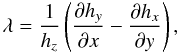
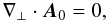
We define the coronal part above an active region in terms of the bounded computational box Ωb = [x0,x1] × [y0,y1] × [0,z1] . The boundary ∂Ωb has two parts: the first, Sp = ∂Ωb ∩ {z = 0}, lies in the plane {z = 0} and represents the photospheric part of the region, while the second, Sn = ∂Ωb \ Sp, is introduced for numerical necessity. We denote as n̂ the inner unit normal to ∂Ωb, such that n̂ = ẑ on Sp.
The standard Grad-Rubin iterative algorithm for computing the force-free magnetic field
B in Ωb is defined by a couple of hyperbolic
and elliptic BVPs given by: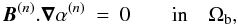 (1)
(1)
 (2)and
 (3)
(3)
 (4)
(4)
 (5)
(5)
The iteration process is initialized by choosing for B(0) the unique solution of
 (6)
(6)
 (7)
(7)
 (8)
(8)
where
hn and λ are the given boundary values for
Bn = B·n̂
and α, respectively, and  is the part of
∂Ωb where
hn > 0. Alternatively, the value of
α(n) may be fixed onto the part
is the part of
∂Ωb where
hn > 0. Alternatively, the value of
α(n) may be fixed onto the part
 of
∂Ωb where
hn < 0. There are thus two possible
versions of GRBVP, to which we refer hereafter as GR+ and GR−,
respectively. On the one hand, GR+ was solved in Amari et al. (2006) by the code XTRAPOL, which uses a vector potential to insure
the divergence-less constraint, and on the other hand by the code FEMQ, which dealt with
that constraint using a least squares method minimising ∇·B.
of
∂Ωb where
hn < 0. There are thus two possible
versions of GRBVP, to which we refer hereafter as GR+ and GR−,
respectively. On the one hand, GR+ was solved in Amari et al. (2006) by the code XTRAPOL, which uses a vector potential to insure
the divergence-less constraint, and on the other hand by the code FEMQ, which dealt with
that constraint using a least squares method minimising ∇·B.
Because of the observational constraints, however, the methods used in Amari et al. (2006) are affected by limitations when applied to reconstruct the field of an actual active region. We now examine these limitations.
2.2. Boundary conditions for Bn and α
In the elliptic BVP above, hn is assumed to be given on the six faces. Observations however only provide hn on the lower face Sp. This leads us to ask: How we can use these limited data in the reconstruction method?
For the hyperbolic part of GR+, the boundary condition on
α(n) is fixed to be on
 . The algorithm first computes
the characteristics
X(n)(r,s)
of B(n) passing through
r ∈ Ωb as the solution of
. The algorithm first computes
the characteristics
X(n)(r,s)
of B(n) passing through
r ∈ Ωb as the solution of
![Mathematical equation: \begin{eqnarray} \label{Equfline1} [\bX^{(n)}]' &=& \B^{(n)}(\bX^{(n)}) , \end{eqnarray}](/articles/aa/full_html/2010/14/aa13058-09/aa13058-09-eq44.png) (9)
(9)
 (10)
(10)
where the prime symbol represents differentiation with respect to the parameter s that runs along the characteristic. The value of α(n) at r is thus set equal to
![Mathematical equation: \begin{eqnarray} \alpha^{(n)}(\r) = \lambda[\bX^{(n)}_{+}(\r)] , \label{Equalphanum1} \end{eqnarray}](/articles/aa/full_html/2010/14/aa13058-09/aa13058-09-eq48.png) (11)
(11)
where
we use the notation  for the
footpoints of the characteristic X on the positive and
negative polarity parts of the boundary, respectively.
for the
footpoints of the characteristic X on the positive and
negative polarity parts of the boundary, respectively.
On , λ can be
evaluated from the measured magnetic field h by using the
relation
 (12)
(12)
and
Eq. (11) can be immediately used when
 . But a problem arises when
 , as we have no observed
value λ at that point. We are thus faced with the following question:
Which value should be attributed to
α(n)(r)
in that situation? In Amari et al.
(2006), this problem did not occur because the two computational methods were
tested only in cases where λ is given on the whole
∂Ωb. A simple possibility, adopted in Amari et al. (1999), consists of imposing
α(n) = 0 at those locations, but this
leads to zero electric current along the associated characteristics, and then to a
magnetic field with an energy lower than the energy of the actual field.
, as we have no observed
value λ at that point. We are thus faced with the following question:
Which value should be attributed to
α(n)(r)
in that situation? In Amari et al.
(2006), this problem did not occur because the two computational methods were
tested only in cases where λ is given on the whole
∂Ωb. A simple possibility, adopted in Amari et al. (1999), consists of imposing
α(n) = 0 at those locations, but this
leads to zero electric current along the associated characteristics, and then to a
magnetic field with an energy lower than the energy of the actual field.
2.3. Photospheric measurement errors and non force-free boundary
We consider a characteristic
X(r,s) of
the field computed by GR+, and assume that it connects
to and then carries a value of
α equal to the value of λ at its footpoint on
. Regardless of the methods
used to answer the two questions above, this value is most generally expected to differ
somewhat from the value of λ given at its computed footpoint on
by the measurements. This is
due to the various reasons already enumerated in the introduction: observational errors in
the measurements of h, likely importance of the nonmagnetic
forces in the layer where the measurements are effected, and, to a lesser extent, in the
corona itself. In other words, the observational data
(hz,λ) on
Sp are most generally inconsistent with each
other. They are not even expected to satisfy the necessary condition of
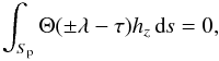
compatibility (Aly 1989)
 (13)
(13)
where
Θ is the standard Heaviside function and τ ≥ 0 an arbitrary number (this
constraint is exact only if we consider Ωb to be the whole half-space
{z > 0}, although it has to still hold true
for some range of sufficiently large values of τ in the general situation
where the larger values of λ are reached in the central part of
Sp). The discrepancy between the computed and measured
values of α on may be
estimated by the number
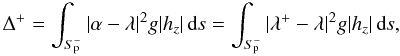 (14)
(14)
where λ + (r) = λ [X±(r)] and g|hz| > 0 is some weight function introduced to take into account the degree of confidence one may have in the accuracy of the data. A proper choice may actually be g = 1, which places more weight on the regions of strong fields where the measurements of λ are more reliable. The reconstruction may clearly be considered to be of some value only if
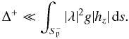 (15)
(15)
The same line of arguments of course, applies (up to a change in signs) if we consider GR− instead of GR+.
If we apply both methods GR± to the same data, we can a posteriori compare the
number Δ± and select the reconstruction that provides the smallest error.
Continuing this line of thought a little further, one may also ask whether it
would be possible to diminish some quadratic distance between the measured
values λ and the computed ones on the whole
Sp by imposing
α in the formulation of GRBVP to take on
a value λ1 ≠ λ, but as
close as possible to λ?
We note that this question relates to the idea of preprocessing the data, which has been used in relation to the optimization methods of reconstruction (Wiegelmann et al. 2006). Preprocessing consists of modifying as little as possible (in some sense) the actual data h to make them satisfy some necessary global constraints of compatibility (Aly 1989). A simple preprocessing of the values of λ may consist here of requiring λ1 to satisfy the set of constraints presented in Eq. (13). This operation, however, appears to be difficult to implement even if we restrict ourselves to a small number of values of τ, and we proceed in a somewhat simpler way in the next section.
3. The optimization Grad-Rubin method (OGRM)
We now present our revisited Grad-Rubin type algorithm (OGRM), which gives a possible solution to the issues discussed in the previous section.
3.1. Boundary condition for Bn
In all cases, we assume that on the horizontal rectangle Sp, the function hn is given by the observations and takes the value hn = hz .
For the “numerical” boundary Sn, a possible (and most common) choice would be to insist that
 (16)
(16)
which
of course is allowed only if the magnetic flux  (if this is not the case, our reconstruction
scheme could be applied only after preprocessing the
hz-data to ensure that the total flux
vanishes). With the boundary condition Eq. (16) being enforced, the magnetic lines of the force-free field
B do not go across Sn and
magnetic connections between the domain to which reconstruction is applied and its
environment are thus not allowed. This may be an unwanted feature as this domain is most
generally non magnetically isolated, either because the part
Sp of the photosphere over which data are available does not
cover all the active region to which it belongs, or because it is connected by bundles of
magnetic lines to other regions. Moreover, this assumption makes the computed field
certainly more compressed than the actual one, which may lead to an overestimate of the
magnetic energy.
(if this is not the case, our reconstruction
scheme could be applied only after preprocessing the
hz-data to ensure that the total flux
vanishes). With the boundary condition Eq. (16) being enforced, the magnetic lines of the force-free field
B do not go across Sn and
magnetic connections between the domain to which reconstruction is applied and its
environment are thus not allowed. This may be an unwanted feature as this domain is most
generally non magnetically isolated, either because the part
Sp of the photosphere over which data are available does not
cover all the active region to which it belongs, or because it is connected by bundles of
magnetic lines to other regions. Moreover, this assumption makes the computed field
certainly more compressed than the actual one, which may lead to an overestimate of the
magnetic energy.
Another possibility would be to assume that
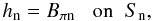 (17)
(17)
with the potential field Bπ(x,y,z) = ∇Vπ(x,y,z) being computed by solving the BVP
 (18)
(18)
 (19)
(19)
 (20)
(20)
set in the whole half-space. The solution can be written in the explicit form
 (21)
(21)
and is valid even when the photospheric flux is non-zero (in the latter case, Bπ has open lines extending to infinity). In contrast to the first choice: (i) this one leads to a non-zero hn on Sn, and allows the computation of a magnetic field and its associated current, which may enter or leave Ωb across Sn; (ii) the computed field is minimally confined as Bπ expands into the whole half-space, while being generated by a hz vanishing outside Sp.
Instead of one of the two conditions above, we choose the boundary condition
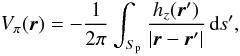
 (22)
(22)
with the potential field Bπ(x,y,z) = ∇Vπ(x,y,z) now being computed by solving the mixed (Neumann-Dirichlet) BVP
 (23)
(23)
 (24)
(24)
 (25)
(25)
As the previous one, this choice of hn allows the field and the current to cross Sn. This may be considered here to be a direct consequence of the last boundary condition, Eq. (25), which causes Bπ to be normal to Sn. From the point of view of the confinement of B in Ωb, this property may be expected to make the computed field (whose lines will actually be no longer strictly normal to Sn) somewhere between those computed with the two first choices of hn, and it may be argued that the action exerted on the field by the magnetic environment of the region is to some extent more accurately taken into account than it is with the two first choices of hn. We add finally that previous test cases have shown that the present choice of hn on Sn provides optimal results for the reconstructed field when combined with a method for fixing the boundary condition on α, which allows current to flow through Sn. It is quite possible, however, that the improvement is due mainly to the latter factor.
3.2. Computation of the vector potential
In our code XTRAPOL, the condition ∇·B(n) = 0 is imposed by introducing a vector potential A(n) and ensuring that the iterated field B(n) = ∇ × A(n). A(n) satisfies the gauge and boundary conditions
 (26)
(26)
 (27)
(27)
where Aπ is a specific vector potential of the potential field Bπ such that ∇·Aπ = 0, and Xt denotes the component of X tangential to the boundary. In Amari et al. (2006), Aπ was uniquely fixed by the boundary condition ∇t·Aπt = 0 on ∂Ωb. Its computation from hn thus required us to solve a 2D Poisson equation on that entire surface, considered as a single 2D domain, with the continuity of At at the edges being ensured by solving an asymmetric linear system. This method proved to be efficient for the test cases (reconstruction of an analytically known force-free field), but we found that the convergence of the algorithm was sensitive to data smoothness when considering true active regions. We therefore modify the computation of Aπt to develop a much more robust method.
In our new scheme, Aπ is constructed as follows. It must satisfy the gauge condition Aπz = 0, and thus be of the general form (DeVore 2000)
 (28)
(28)
The lower boundary value A0(x,y) = Aπ(x,y,0) must satisfy
 (29)
(29)
(where ∇ ⊥ = x̂∂x + ŷ∂y) and is defined only up to the addition of the gradient of an arbitrary function f(x,y). To fix this remaining gauge arbitrariness, we also impose
 (30)
(30)
which implies, along with the equation ∇ × Bπ = 0, the required condition
 (31)
(31)
There does clearly exist a function χπ(x,y,z) such that
 (32)
(32)
where χπ satisfies the relation
 (33)
(33)
and χ(x,y) = χπ(x,y,0), which can be readily applied to solve the equation
 (34)
(34)
To determine effectively Aπ on ∂Ωb, we proceed as follows. We first compute the function χπ(x,y,0) in Sp by solving the 2D Poisson equation given by Eq. (34) (with z = 0) with the boundary condition
 (35)
(35)
We thus obtain Aπ(x,y,0) = ∇χπ(x,y,0) × ẑ. We next use Eq. (28) and the values of Aπ on ∂Sp to derive Aπ on the vertical part of ∂Ωb. We finally obtain Aπ(x,y,z1) by solving Eq. (34) (now with z = z1) along with the Neumann boundary condition ∂nχπ(x,y,z1) = (n̂ × ẑ)·Aπ on the boundary of the upper face (where Aπ is known from the previous step). We note that Aπ is tangential to ∂Ωb: as a mere consequence of the gauge condition Aπz = 0 on the lower and upper horizontal faces, and as a consequence of Eqs. (33), (35), and (25) on the vertical ones.
3.3. Boundary condition for α
To start with, we define the error functional
![Mathematical equation: \begin{eqnarray} \cO[\B,\mu;g] = \int_{\S_{\rm p}}\abs{\mu-\lambda}^{2}g\abs{B_{z}}\is , \label{DefO} \end{eqnarray}](/articles/aa/full_html/2010/14/aa13058-09/aa13058-09-eq123.png) (36)
(36)
which is used to measure the closeness between the boundary values imposed on α and the measured values λ. In that expression, B is an arbitrary magnetic field in Ωb (with Bn = hn on ∂Ωb), μ is an arbitrary function defined on ∂Ωb taking the same value at both footpoints of an arbitrary line of B, i.e.,
 (37)
(37)
and g|Bz| ≥ 0 is some fixed weight function (as in Eq. (14), the factor |hz| has been singled out for convenience). This weight function is supposed to represent the confidence that can be placed on the values of λ computed from the three components of the measured field, and thus must be fixed on the basis of instrumental considerations (not discussed here). Quite naturally, we extend g to the whole ∂Ωb by setting g = 0 on Sn, where no observational data are available.
By flux conservation along a thin flux tube, we have
(Bnds)(r) = −(Bnds)(X±(r)))
for  , and can
rewrite the functional O in the form
, and can
rewrite the functional O in the form
![Mathematical equation: \begin{eqnarray} \cO[\B,\mu;g] = \int_{\partial\Omega_{\rm b}^{+}}\left[\abs{\mu-\lambda}^{2}g + \abs{\mu-\Lambda}^{2}G\right]\abs{B_{\rm n}}\is , \label{DefO1} \end{eqnarray}](/articles/aa/full_html/2010/14/aa13058-09/aa13058-09-eq134.png) (38)
(38)
where
we have set
(G,Λ)(r) = (g,λ)(X−(r)))
for  , and λ has
been extended in an arbitrary way to
, and λ has
been extended in an arbitrary way to  (where
g = 0). By developing the squares in the integrand in the right-hand
side of Eq. (38) and by rearranging the
terms, we derive the alternative formula
(where
g = 0). By developing the squares in the integrand in the right-hand
side of Eq. (38) and by rearranging the
terms, we derive the alternative formula
![Mathematical equation: \begin{eqnarray} \cO[\B,\mu;g] &=& \int_{S^{+}}\left[(g+G)\left(\mu -\unmu\right)^{2} + \frac{gG}{g+G}(\lambda-\Lambda)^{2}\right]\abs{B_{z}}\is \nonumber \\ \label{DefOa} &\geq& \int_{S^{+}}\frac{gG}{g+G}(\lambda-\Lambda)^{2}\abs{B_{z}}\is , \end{eqnarray}](/articles/aa/full_html/2010/14/aa13058-09/aa13058-09-eq138.png) (39)
(39)
where
we have introduced the function  defined on
by
defined on
by
 (40)
(40)
It
is then quite clear that, for fixed magnetic field B and
boundary data λ,
O [B,μ;g] is
minimized by the function , with its minimum value being
given by
![Mathematical equation: \begin{eqnarray} \underline{O}[\B;g] = \cO[\B,\unmu;g] = \int_{\partial\Omega_{\rm b}^{+}} \frac{gG}{g+G}(\lambda-\Lambda)^{2}\abs{B_{\rm n}}\is . \end{eqnarray}](/articles/aa/full_html/2010/14/aa13058-09/aa13058-09-eq142.png) (41)
(41)
The latter is to be compared with the value
![Mathematical equation: \begin{eqnarray} \cO[\B,\mu_{0};g] = \int_{\partial\Omega_{\rm b}^{+}} G(\lambda-\Lambda)^{2}\abs{B_{\rm n}}\is , \end{eqnarray}](/articles/aa/full_html/2010/14/aa13058-09/aa13058-09-eq143.png) (42)
(42)
assumed
by O when we take for μ the function
μ0 satisfying
μ0 = λ on . We note that a standard
variational argument applied to Eq. (38)
would have given immediately as an extremizer, but some more
work would then have been needed to demonstrate that ![Mathematical equation: $\cO[\B,\unmu;g]$](/articles/aa/full_html/2010/14/aa13058-09/aa13058-09-eq146.png) is a minimum.
is a minimum.
To obtain a possible solution to the third question addressed in the previous section, we
now introduce the optimization-Grad-Rubin problem (OGRP), for which we
attempt to determine a couple of terms
(B,α) in
Ωb satisfying the equations and boundary conditions of the
standard Grad-Rubin problem, but with a boundary condition for
α on  that is self-consistently determined in such a way that the functional
O [B,α;g]
takes its lowest possible value.
that is self-consistently determined in such a way that the functional
O [B,α;g]
takes its lowest possible value.
Equation (40) suggests trying to solve OGRP by using a simple modification of the standard Grad-Rubin iterative scheme into which we could substitute the boundary condition given by Eq. (2) by
 (43)
(43)
where
 and we recall that
X(n)(r,s)
denotes the characteristics associated with
B(n). We note that the
boundary condition changes at each iteration step, and that OGRM is based on a
coprocessing of the boundary data on λ, in contradistinction to an a
priori preprocessing such as that used in Wiegelmann
et al. (2006). The jump from GR± to OGRM clearly does not entail many
complications. In the modified scheme, we have to extend the line through each point
r in Ωb in both directions (towards
and
and we recall that
X(n)(r,s)
denotes the characteristics associated with
B(n). We note that the
boundary condition changes at each iteration step, and that OGRM is based on a
coprocessing of the boundary data on λ, in contradistinction to an a
priori preprocessing such as that used in Wiegelmann
et al. (2006). The jump from GR± to OGRM clearly does not entail many
complications. In the modified scheme, we have to extend the line through each point
r in Ωb in both directions (towards
and  ), while
we had to do this in only one direction (towards ) when
dealing with the standard scheme.
), while
we had to do this in only one direction (towards ) when
dealing with the standard scheme.
The condition illustrated by Eq. (43) may
be detailed as follows. Firstly when both footpoints of
X(n)(r,s)
are located on Sp, this characteristic receives a value of
α(n), which is some average between the
values of λ at  and
and
 , respectively. If
we choose for instance g = 1 on Sp, we find
that
, respectively. If
we choose for instance g = 1 on Sp, we find
that
 (44)
(44)
which
is merely the arithmetic mean of the values of λ at its footpoints. A
similar value appears in Inhester & Wiegelmann
(2006), but with a somewhat different justification. Secondly when
X(n)(r,s)
connects (where
g = 0) to , it
receives the value
α(n) = Λ(n),
i.e.,
![Mathematical equation: \begin{eqnarray} \alpha^{(n)}(\r) = \lambda[\bX_{-}^{(n)}(\r)] . \label{Equalphanum2} \end{eqnarray}](/articles/aa/full_html/2010/14/aa13058-09/aa13058-09-eq157.png) (45)
(45)
OGRM
thus also answers the second question set in Sect. 2.2. We note that it provides in general a nonzero value for
α(n) on the characteristics entering
Ωb through .
We conclude this section by pointing out the main difference between our method for
taking into account the values of λ on the whole
Sp and the method proposed by Wheatland & Regnier (2009). We reach our final force-free field
after a single series of iterations, but Wheatland
& Regnier (2009) require a double series of iterations to obtain theirs.
They indeed compute a sequence of force-free fields by alternatively solving either a
GR+ or a GR−. More precisely, they start with the computation of a
force-free field B1 by GR+, i.e., by
using the values of λ on . A field
B2 is thus computed by GR−, with
the boundary values of α on being taken to be equal to
some average between the observational values λ and the values of
α1 computed at the previous step. The process is thus
reiterated until convergence of the sequence
{Bk} is obtained.
 |
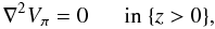
Fig. 1 Distributions on Sp of Bz and λ = αExact for the reference case FFF1(0). |
4. Test cases
4.1. General method
We check the effectiveness of OGRM by computing a series of test cases performed with a
numerical resolution of 643. Since OGRM depends on the choice of a function
g, we denote it as OGRM(g) hereafter because two
different choices of g are under simultaneous consideration. We note that
GR± may be considered to be OGRM(g±),
respectively, where g± = 1 on  , and
g± = 0 on
, and
g± = 0 on  .
.
As in Amari et al. (2006), we use for our tests a particular analytical force-free field that belongs to the well-known class derived in Low & Lou (1990, referred to hereafter as LowLou solution). This solution is defined by the parameters FFF1: = (n = 1,m = 1,L = .3,Φ = π / 4). As OGRM may differ significantly from GR± only when the boundary data are not compatible, we construct an “observed” function λ by perturbing the exact boundary value αexact taken on Sp by the analytic α-function. We use two types of perturbations – nonrandom and random, respectively –, each one being supposed to represent some errors in the photospheric measurements. For each data set obtained in this way: (i) we reconstruct the field using four methods: GR+, GR−, OGRM(g = 1), and OGRM(g = |Bn|-1); (ii) we analyse their convergence by considering the behaviours of the quantity
 (46)
(46)
and the norm ||B(n)||L2, where
 (47)
(47)
(iii) we compare the values taken by the error functional O [g] in which we take successively g = 1 and g = |Bn|-1. Our choices of g are somewhat arbitrary, being made here just for convenience, and we do not claim that they are the relevant ones for applications to actual data (rather, the choice of g for a set of actual data should be made after a thorough analysis of the observational errors, ...). We note that it makes sense to evaluate O [g] even for a solution computed with OGRM(g'), with g' ≠ g. In O [g], the weight g is determined by the quality of the observations, and once it has been fixed, O [g] may be used to evaluate the quality of a solution obtained from the data (hn,λ) by any means – e.g., by using OGRM [g'] . Of course, what we wish to check is that the optimal result – i.e., the lowest value of O [g] – is obtained for OGRM(g). Finally, we also point out that the reconstruction of a perturbed state even with GR+ and GR−, constitutes a test of the continuity of the solutions with respect to changes in the boundary conditions (i.e., one of the conditions for having a well-posed problem).
 |
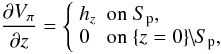
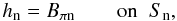
Fig. 2 Convergence properties of the four methods GR+, GR−, OGRM(g = 1), and OGRM(g = |Bn|-1), in the reference case FFF1(0). The convergence rate is fast and the norm of the solution reaches its asymptotical value in about 15 iterations, apart from the case of OGRM(g = 1), which converges at a slightly lower rate requiring about 30 iterations. |
4.2. Reference case
As a preliminary test, we first consider the case (referred to as FFF1(0)) defined by the boundary condition λ = αExact on Sp, for which we should ideally expect the four methods to lead to the exact force-free LowLou solution. However, as noticed in Amari et al. (2006), some errors caused by the discretisation and interpolation on the computational grid cannot be completely eliminated, and we already have a situation where small departures from compatibility are present. Figure 1 shows the distributions of Bz and λ on Sp for this reference case.
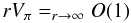
As can be seen in Fig. 2, and as expected, the four methods converge rapidly for this unperturbed case, although at a somewhat lower rate for OGRM(g = 1). Figure 3 also shows that they behave almost identically, reaching in particular the same value of O.
 |
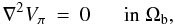
Fig. 3 Error functionals O(g = 1) and O(g = |Bn|-1), for the four methods GR+, GR−, OGRM(g = 1), and OGRM(g = |Bn|-1), applied to the reference case FFF1(0). The four methods lead to almost the same small value for these errors, with a slight advantage for OGRM(g = 1) and OGRM(g = |Bn|-1). |
4.3. Nonrandom perturbation
We next consider a boundary function λ obtained from αExact by applying a specific nonrandom perturbation. The new λ, which defines the case FFF1(t+,t−), is given by
 (48)
(48)
 (49)
(49)
where t± and t− are real numbers in [0,1 [.
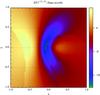 |
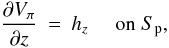
Fig. 4 Distribution on Sp of λ(0.15,0.15) obtained by perturbing αExact in a nonrandom way. |
We first consider the symmetric case FFF1(0.15,0.15), whose corresponding λ(0.15,0.15) on Sp is shown in Fig. 4. As can be seen in Fig. 5, the four methods lead once more to a low value of the convergence parameter η(n), with the smallest value being obtained for OGRM(g = 1).
It is also clear in Fig. 6, which shows the two error functionals O(g = 1) and O(g = |Bn|-1), that the two methods OGRM(g = 1) and OGRM(g = |Bn|-1) lead to smaller errors than those obtained with GR+ and GR− (although with a lower difference for the latter).
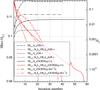 |
Fig. 5 Convergence properties of the four methods GR+, GR−, OGRM(g = 1), and OGRM(g = |Bn|-1), in the non randomly perturbed case case FFF1(.15,.15). The convergence rate is fast, even if lower for OGRM(g = 1). |
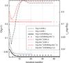 |
Fig. 6 Error functionals O(g = 1) and O(g = |Bn|-1) for the four methods GR+, GR−, OGRM(g = 1), and OGRM(g = |Bn|-1), applied to the non randomly perturbed case FFF1(.15,.15). The optimal results are obtained with OGRM(g = 1), OGRM(g = |Bn|-1), and OGRM(g = |Bn|-1), which is even slightly better. |
For the case FFF1(0.1,0.4) corresponding to the asymmetric
choice of parameters t± = 0.1 for and
t− = 0.4 on in Eq. (49) defining our non randomly perturbed
boundary condition, the corresponding
λ(0.1,0.4) is shown in Fig. 7. The four methods converge at about the same fast rate,
as shown in Fig. 8, but the difference in behaviour
is accentuated (see Fig. 9). Indeed, while the two
weighted methods are clearly better than the original GR+ and GR−,
OGRM(g = |Bn|-1) infers
lower error values than OGRM(g = 1). This shows the effect of the weight
in our method.
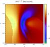 |
Fig. 7 Distribution of
λ(.1,.4)
obtained from αExact by a nonrandom perturbation defined
by the parameters t± = 0.1 in
|
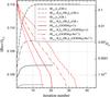 |
Fig. 8 Convergence properties of the four methods GR+, GR−, OGRM(g = 1), and OGRM(g = |Bn|-1), applied to the non randomly perturbed case case FFF1(.1,.4). |
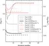 |
Fig. 9 Error functionals O(g = 1) and O(g = |Bn|-1) for the four methods GR+, GR−, OGRM(g = 1), and OGRM(g = |Bn|-1), in the non randomly perturbed case FFF1(.1,.4). The best results are obtained with OGRM(g = |Bn|-1). |
4.4. Random perturbation
We finally apply to the reference boundary function αExact a random perturbation that produces a λ of the form
 (50)
(50)
 (51)
(51)
where
Random is a random function taking its values in
[0,1], and δ is a positive coefficient controlling
the magnitude of the perturbation. The perturbation can thus take both signs on
S, with no special correlation between its values on
or . We refer to the corresponding
randomly perturbed state as FFF1(δ), and consider two
particular values of δ.
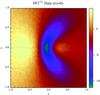 |
Fig. 10 Distribution of λ(1) obtained from αExact by a random perturbation defined by Eq. (51) with δ = 1. |
As can be seen in Fig. 10, the random perturbation is relatively moderate in the FFF1(1) case. Moreover, one can already see that the four methods converge rapidly, with a lower rate for OGRM(g = 1), while OGRM(g = |Bn|-1) converges almost as rapidly as the original GR+ and GR−. By inspecting the error functional diagnostics shown in Fig. 11, we see that the four methods perform almost identically well, with a slight superiority for the two weighted methods.
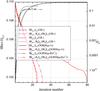 |
Fig. 11 Convergence properties of the four methods GR+, GR−, OGRM(g = 1), and OGRM(g = |Bn|-1), applied to the randomly perturbed case case FFF1(1). |
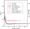 |
Fig. 12 Error functionals O(g = 1) and O(g = |Bn|-1) for the four methods GR+, GR−, OGRM(g = 1), and OGRM(g = |Bn|-1), applied to the randomly perturbed case FFF1(1) . The best results are obtained with OGRM(g = |Bn|-1). |
We finally consider the randomly perturbed case FFF1(10) corresponding to the strong perturbation seen in Fig. 13. The four methods converge to different values (see Fig. 14), with the smallest values being found for GR+ and GR−. The values reached by OGRM(g = 1) and OGRM(g = |Bn|-1), although larger, can be considered as accurate for such a strong perturbation. The error functional diagnostics gathered in Fig. 15 clearly show that OGRM(g = |Bn|-1) provides the lowest error. This clearly shows that in the case of a strong perturbation the choice of weight g = |Bn|-1) leads to a lower error (in the sense explained above) than the choice corresponding to g = 1.
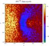 |
Fig. 13 Distribution on Sp of λ(10) obtained from αExact by a random perturbation defined by Eq. (51) with δ = 10. |
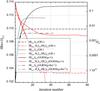 |
Fig. 14 Convergence properties of the four methods GR+, GR−, OGRM(g = 1), and OGRM(g = |Bn|-1), applied to the randomly perturbed case FFF1(10). |
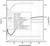 |
Fig. 15 Error functionals O(g = 1) and O(g = |Bn|-1) for the four methods GR+, GR−, OGRM(g = 1), and OGRM(g = |Bn|-1), applied to the randomly perturbed case FFF1(10). The best results are obtained with OGRM(g = |Bn|-1). |
5. Conclusion
We have addressed some issues that arise when one wishes to reconstruct the field of a coronal active region using one of our previously presented Grad-Rubin type schemes (Amari et al. 2006) and observationally acquired data. A first issue is related to the computations always being performed in a finite box: this introduces an artificial “numerical boundary” over which the observations which are obtained only at the photospheric level, do not furnish the required boundary conditions for both the normal component of the field and the force-free function α. The problem is thus to account in some way for this lack of data. The second issue arises from the values of Bn and α measured at the photospheric level never being “compatible” because of the errors in the observations and their treatment (e.g., in the disambiguation of the transverse field), and because the actual field is far from being force-free in the photospheric layers, and not even exactly force-free in the corona. A disagreement is found when the field is reconstructed by one of our earlier methods – either GR+ or GR−: the values of α computed in the polarity where this quantity is not imposed do not match those measured in this polarity. Here the problem one is naturally led to face is what is the most accurate determination of the boundary condition on α to be used in the hyperbolic part of GRBVP.
We have proposed to answer the two questions above by introducing a new method,
OGRM(g), where g is some weight function. In
OGRM(g), the value of Bn on the “numerical
part” Sn of the boundary is constrained to be equal to that of
the potential field computed as follows: its normal component is constrained to be equal to
the measured one on the photospheric part Sp of the boundary,
while its tangential component vanishes on Sn. This choice is in
some sense intermediate between two other more common choices, the one in which the
potential field is fully confined inside the numerical box, and the one in which this field
is allowed to fully expand into the whole half-space. As the latter, it allows the field and
the current to go across the numerical boundary, which is most generally a desirable feature
because the region whose field is reconstructed is not magnetically isolated from its
environment. As for the boundary condition imposed on α, it is selected in
OGRM(g) by trying to minimize an error functional (depending on
g) measuring the difference between the computed boundary values of
α and the measured ones. This selection cannot be made a priori, as the
error functional depends on the field that has to be computed. But we have shown
mathematically that it is possible to make that choice in a step by step way, by setting up
a new Grad-Rubin type algorithm. In OGRM, at each iteration α is assumed to
be equal to some weighted average of the values measured at both the footpoints of a line
(or the value taken at its photospheric footpoint when one footpoint lies on the numerical
boundary). This method is in some sense midway between the optimization methods that use all
the available data but cannot compute from them an exact force-free field, and the
Grad-Rubin ones that use only half of the data (Bn being fixed
on ∂Ωb, and α on either
or ) to
compute an exactly force-free field. Compared to GR± developed in Amari et al. (2006), OGRM(g) does not
require either far more iterations or a new internal iteration loop. Moreover, it does not
distinguish between the solutions obtained by imposing α on the positive
and negative polarity, respectively. In that sense OGRM(g) is symmetric by
construction, and is based on a unique BVP. As we have already pointed out, it is not the
first time that the values of α measured over the whole photospheric
boundary are used as an input for a Grad-Rubin scheme. Proposals have already been made by
Inhester & Wiegelmann (2006) and by Wheatland & Regnier (2009), which differ from
ours in one way or another.
We have applied OGRM(g) to a series of test cases in which the “photospheric” values of α are obtained by perturbing the αExact provided by a LowLou force-free field. We have used two types of perturbations, random and nonrandom, and used for both the reconstruction and the error functional, two different weight functions: (i) g = 1, which corresponds to substituting into the error functional an actual weight g|Bn| = |Bn| that provides greater importance to the high field regions, and attributes to each characteristic a value of α equal to the arithmetic average
of the values measured at its footpoints when both lie in the photosphere; (ii)
 , which corresponds to an
actual weight function g|Bn| = 1 in the
error functional and thus appears to place all the regions on the same footing. These
somewhat arbitrary choices proved to be adequate for testing the convergence and efficiency
of OGRM(g). But for the reconstruction of the field of an actual active
region, a thorough analysis of the observational conditions in which the data have been
obtained is of course necessary to determine g. The latter depends on
quantities such as the norm of the transverse field and the magnitude of the polarisation
errors (as in the “stress and relax” method of Roumeliotis
1996), and are set to zero where data are of particularly poor quality, ... The new
scheme OGRM(g) has been found to have convergence properties comparable to
those of the old ones, GR±. It is just a bit slower (requiring more iterations),
which should be related to the boundary condition on α changing at each
step. The best results (in the sense of minimisation of error functional) have been obtained
with OGRM
, which corresponds to an
actual weight function g|Bn| = 1 in the
error functional and thus appears to place all the regions on the same footing. These
somewhat arbitrary choices proved to be adequate for testing the convergence and efficiency
of OGRM(g). But for the reconstruction of the field of an actual active
region, a thorough analysis of the observational conditions in which the data have been
obtained is of course necessary to determine g. The latter depends on
quantities such as the norm of the transverse field and the magnitude of the polarisation
errors (as in the “stress and relax” method of Roumeliotis
1996), and are set to zero where data are of particularly poor quality, ... The new
scheme OGRM(g) has been found to have convergence properties comparable to
those of the old ones, GR±. It is just a bit slower (requiring more iterations),
which should be related to the boundary condition on α changing at each
step. The best results (in the sense of minimisation of error functional) have been obtained
with OGRM , which
proved to be the most robust method corresponding to the lowest discrepancies between the
measured values of α and the computed ones on the photospheric boundary.
, which
proved to be the most robust method corresponding to the lowest discrepancies between the
measured values of α and the computed ones on the photospheric boundary.
We note that we do not claim that OGRM solves the issue related to the non force-free character of the magnetic field in the layer where it is measured: OGRM just provides a possible way of using as well as possible the data obtained by the currently available instruments. The “non force-free” issue is common to all the force-free reconstruction methods, and its solution is likely to require the construction of a more general class of models in which both the corona and a subphotospheric layer are treated in similar ways.
Acknowledgments
We are grateful to the referee, B. Inhester, for his constructive comments, which led to an improved version of the paper. T.A. thanks A. Canou for discussion. We would also like to thank the Centre National d’Études Spatiales (CNES) for support.
References
- Aly, J.-J. 1989, Sol. Phys., 120, 19 [NASA ADS] [CrossRef] [Google Scholar]
- Aly, J.-J., & Amari, T. 2007, Geophys. Astrophys. Fluid Dyna., 101, 249 [Google Scholar]
- Amari, T., Boulmezaoud, T. Z., & Mikic, Z. 1999, A&A, 350, 1051 [NASA ADS] [Google Scholar]
- Amari, T., Boulmezaoud, T. Z., & Aly, J.-J. 2006, A&A, 446, 691 [NASA ADS] [CrossRef] [EDP Sciences] [Google Scholar]
- DeVore, C. R. 2000, ApJ, 539, 944 [NASA ADS] [CrossRef] [Google Scholar]
- Inhester, B., & Wiegelmann, T. 2006, Sol. Phys., 235, 201 [NASA ADS] [CrossRef] [Google Scholar]
- Low, B. C., & Lou, Y. Q. 1990, ApJ, 352, 343 [NASA ADS] [CrossRef] [Google Scholar]
- Mikic, Z., & McClymont, A. N. 1994, in Solar Active Region Evolution: Comparing Models with Observations, ed. K. S. Balasubramaniam, & G. W. Simon, ASP Conf. Ser., 68, 225 [Google Scholar]
- Roumeliotis, G. 1996, ApJ, 473, 1095 [NASA ADS] [CrossRef] [Google Scholar]
- Sakurai, T. 1981, Sol. Phys., 69, 343 [NASA ADS] [CrossRef] [Google Scholar]
- Schrijver, C. J., Derosa, M. L., Metcalf, T. R., et al. 2006, Sol. Phys., 235, 161 [Google Scholar]
- Valori, G., Kliem, B., & Keppens, R. 2005, A&A, 433, 335 [NASA ADS] [CrossRef] [EDP Sciences] [Google Scholar]
- Wheatland, M. 2007, Sol. Phys., 245, 251 [NASA ADS] [CrossRef] [Google Scholar]
- Wheatland, M. S., & Régnier, S. 2009, ApJ, 700, L88 [NASA ADS] [CrossRef] [Google Scholar]
- Wiegelmann, T. 2004, Sol. Phys., 219, 87 [NASA ADS] [CrossRef] [Google Scholar]
- Wiegelmann, T. 2008, J. Geophys. Res. (Space Phys.), 113, 3 [Google Scholar]
- Wiegelmann, T., Inhester, B., & Sakurai, T. 2006, Sol. Phys., 233, 215 [NASA ADS] [CrossRef] [Google Scholar]
All Figures
|
Fig. 1 Distributions on Sp of Bz and λ = αExact for the reference case FFF1(0). |
| In the text | |
|
Fig. 2 Convergence properties of the four methods GR+, GR−, OGRM(g = 1), and OGRM(g = |Bn|-1), in the reference case FFF1(0). The convergence rate is fast and the norm of the solution reaches its asymptotical value in about 15 iterations, apart from the case of OGRM(g = 1), which converges at a slightly lower rate requiring about 30 iterations. |
| In the text | |
|
Fig. 3 Error functionals O(g = 1) and O(g = |Bn|-1), for the four methods GR+, GR−, OGRM(g = 1), and OGRM(g = |Bn|-1), applied to the reference case FFF1(0). The four methods lead to almost the same small value for these errors, with a slight advantage for OGRM(g = 1) and OGRM(g = |Bn|-1). |
| In the text | |
|
Fig. 4 Distribution on Sp of λ(0.15,0.15) obtained by perturbing αExact in a nonrandom way. |
| In the text | |
|
Fig. 5 Convergence properties of the four methods GR+, GR−, OGRM(g = 1), and OGRM(g = |Bn|-1), in the non randomly perturbed case case FFF1(.15,.15). The convergence rate is fast, even if lower for OGRM(g = 1). |
| In the text | |
|
Fig. 6 Error functionals O(g = 1) and O(g = |Bn|-1) for the four methods GR+, GR−, OGRM(g = 1), and OGRM(g = |Bn|-1), applied to the non randomly perturbed case FFF1(.15,.15). The optimal results are obtained with OGRM(g = 1), OGRM(g = |Bn|-1), and OGRM(g = |Bn|-1), which is even slightly better. |
| In the text | |
|
Fig. 7 Distribution of
λ(.1,.4)
obtained from αExact by a nonrandom perturbation defined
by the parameters t± = 0.1 in
|
| In the text | |
|
Fig. 8 Convergence properties of the four methods GR+, GR−, OGRM(g = 1), and OGRM(g = |Bn|-1), applied to the non randomly perturbed case case FFF1(.1,.4). |
| In the text | |
|
Fig. 9 Error functionals O(g = 1) and O(g = |Bn|-1) for the four methods GR+, GR−, OGRM(g = 1), and OGRM(g = |Bn|-1), in the non randomly perturbed case FFF1(.1,.4). The best results are obtained with OGRM(g = |Bn|-1). |
| In the text | |
|
Fig. 10 Distribution of λ(1) obtained from αExact by a random perturbation defined by Eq. (51) with δ = 1. |
| In the text | |
|
Fig. 11 Convergence properties of the four methods GR+, GR−, OGRM(g = 1), and OGRM(g = |Bn|-1), applied to the randomly perturbed case case FFF1(1). |
| In the text | |
|
Fig. 12 Error functionals O(g = 1) and O(g = |Bn|-1) for the four methods GR+, GR−, OGRM(g = 1), and OGRM(g = |Bn|-1), applied to the randomly perturbed case FFF1(1) . The best results are obtained with OGRM(g = |Bn|-1). |
| In the text | |
|
Fig. 13 Distribution on Sp of λ(10) obtained from αExact by a random perturbation defined by Eq. (51) with δ = 10. |
| In the text | |
|
Fig. 14 Convergence properties of the four methods GR+, GR−, OGRM(g = 1), and OGRM(g = |Bn|-1), applied to the randomly perturbed case FFF1(10). |
| In the text | |
|
Fig. 15 Error functionals O(g = 1) and O(g = |Bn|-1) for the four methods GR+, GR−, OGRM(g = 1), and OGRM(g = |Bn|-1), applied to the randomly perturbed case FFF1(10). The best results are obtained with OGRM(g = |Bn|-1). |
| In the text | |
Current usage metrics show cumulative count of Article Views (full-text article views including HTML views, PDF and ePub downloads, according to the available data) and Abstracts Views on Vision4Press platform.
Data correspond to usage on the plateform after 2015. The current usage metrics is available 48-96 hours after online publication and is updated daily on week days.
Initial download of the metrics may take a while.