| Issue |
A&A
Volume 522, November 2010
|
|
|---|---|---|
| Article Number | A73 | |
| Number of page(s) | 14 | |
| Section | Galactic structure, stellar clusters and populations | |
| DOI | https://doi.org/10.1051/0004-6361/200912733 | |
| Published online | 04 November 2010 | |
Constraining the regular Galactic magnetic field with the 5-year WMAP polarization measurements at 22 GHz
1
Dpto. Física Teórica y del Cosmos. Edif. Mecenas, planta baja, Campus
Fuentenueva, 18071. Universidad de Granada,
Granada,
Spain
e-mail: This email address is being protected from spambots. You need JavaScript enabled to view it.
2
Instituto de Física Teórica y Computacional Carlos I,
Granada,
Spain
3
Instituto de Astrofísica de Canarias (IAC),
C/vía Láctea, s/n, 38200,
La Laguna, Tenerife,
Spain
4
Departamento de Astrofísica, Universidad de La
Laguna, 38205,
La Laguna, Tenerife,
Spain
Received:
19
June
2009
Accepted:
26
June
2010
Abstract
Context. The knowledge of the regular (large scale) component of the Galactic magnetic field gives important information about the structure and dynamics of the Milky Way, and also constitutes a basic tool to determine cosmic ray trajectories. It can also provide clear windows where primordial magnetic fields could be detected.
Aims. We aim to obtain the regular (large scale) pattern of the magnetic field distribution of the Milky Way that better fits the polarized synchrotron emission as seen by the WMAP satellite in the 5 years data at 22 GHz.
Methods. We have done a systematic study of a number of Galactic magnetic field models: axisymmetric (with and without radial dependence on the field strength), bisymmetric (with and without radial dependence), logarithmic spiral arms, concentric circular rings with reversals and bi-toroidal. We have explored the parameter space defining each of these models using a grid-based approach. In total, more than one million models were computed. The model selection was done using a Bayesian approach. For each model, the posterior distributions were obtained and marginalized over the unwanted parameters to obtain the marginal (one-parameter) probability distribution functions.
Results. In general, axisymmetric models provide a better description of the halo component, although with regard to their goodness-of-fit, the other models cannot be rejected. In the case of the disk component, the analysis is not very sensitive for obtaining the disk large-scale structure, because of the effective available area (less than 8% of the whole map and less than 40% of the disk). Nevertheless, within a given family of models, the best-fit parameters are compatible with those found in the literature.
Conclusions. The family of models that better describes the polarized synchrotron halo emission is the axisymmetric one, with magnetic spiral arms with a pitch angle of ≈24°, and a strong vertical field of 1 μG at z ≈ 1 kpc. When a radial variation is fitted, models require fast variations.
Key words: magnetic fields / polarization / Galaxy: structure
© ESO, 2010
1. Introduction
Spiral galaxies exhibit large-scale magnetic fields. The Milky Way is not an exception, but obtaining its spatial distribution is extremely difficult. Most methods for observing magnetic fields are based either on radio observations of the synchrotron emission (Wolleben et al. 2006; Reich 2006; Testori et al. 2008, and references therein), or on the Faraday rotation (hereafter FR) of pulsars (e.g. Weisberg et al. 2004; Han et al. 2006; Noutsos et al. 2008) and extragalactic radio sources (hereafter EGRS) (e.g. Gaensler et al. 2001; Brown et al. 2007; Haverkorn et al. 2008a; Carretti et al. 2008). In addition, several radio lines show Zeeman splitting, which can be used also to directly constrain the strength of the magnetic field (e.g. Fish et al. 2003; Han & Zhang 2007).
Despite the large numbers of pulsars and EGRS for which the rotation measure (hereafter RM) has been recently determined, there is no consensus about the large-scale pattern of the Galactic magnetic field (hereafter GMF). It is probably more complex than previously expected, as pointed out in Men et al. (2008). Recent results by Sun et al. (2008) show an axisymmetric disk distribution with reversals inside the solar circle as the best model to describe the GMF when all-sky maps at 1.4 GHz from DRAO and Villa Elisa, the 22 GHz map from WMAP satellite, and the Effelsberg RM survey of EGRS are combined. Results derived from Brown et al. (2007) by using RM of EGRS suggest an axisymmetric pattern of the disk magnetic field. Vallée (2008) proposed the inclusion of a ring model to describe the field. The interest on the structure of this large scale GMF is justified by a number of reasons. First of all, this field might be important when considering the dynamics of the galaxy at those large scales (Nelson 1988; Battaner et al. 1992; Battaner & Florido 1995; Kutschera & Jalocha 2004; Battaner & Florido 2007). A good characterization of the large-scale GMF pattern would allow a detailed correction of the galactic contribution for a better understanding of cosmological magnetic fields (see Battaner & Florido 2009, for a recent review), which would be potentially observed with upcoming CMB missions such as PLANCK (The Planck Collaboration 2006).
In addition, the GMF modifies the trajectory of high energy cosmic rays, therefore its knowledge is crucial for understanding their distribution in energy and direction, as it is obtained in experiments like Auger (Bluemer et al. 2008), Milagro (Abdo et al. 2009) and others. The global anisotropies found by Milagro have been interpreted by Battaner et al. (2009) as produced by Galactic magnetic fields. Moreover, GMF could be important to explain the well known knee in the spectrum of cosmic rays energies around 106 GeV (Masip & Mastromatteo 2008), because sub-knee-energy cosmic protons trapped by GMF should have a much higher optical depth for interactions with WIMPs.
The extraction of structure of the Galactic magnetic field from the measurements of the polarized intensity is extremely difficult. The Galactic magnetic field probably cannot be described by a single model because there would need to be at least three components, the thin disk, the thick disk (Beuermann et al. 1985) and the halo, each one defined by its own model and parameters. Taking into account that each component is largely unknown, an analysis of a multi-component magnetic field renders an objective estimation of the best configuration a task that is too complicated.
The thin disk is characterized by the highest field strengths, and we are embedded in it. However, magnetic fields in the thin disk are predominantly random, and therefore they barely contribute to the observed net polarized emission, even if a z-component of the regular fields exists (Han et al. 1999). On the other hand, local spurs (Berkhuijsen et al. 1971) like the North Polar Spur, highly distort the main field configuration. Even at this high frequency Faraday depolarization cannot be neglected in particular regions. Observing at high galactic latitudes the thin disk field is contaminated by the thick disk and the halo fields, which could even become dominant. Models for the thick disk are scarce in the literature, but those proposed for the thin disk could be tested, even if different parameters characterized both disks. Our results for the disk inferred from the polarized synchrotron emission will give a complementary insight into the field structure. The halo structure remains unknown and has a very different structure, consisting in a double torus in two hemispheres with opposite directions. After some pioneer detections (Simard-Normandin & Kronberg 1980; Han & Qiao 1994), it has been modeled by Han et al. (1997), Harari et al. (1999), Tinyakov & Tkachev (2002), Prouza & Šmída (2003), and others. To illustrate the current uncertainty on this component, we can compare the maximum value of the magnetic strength, 1 μG following Prouza & Šmída (2003), and 10 μG following Sun et al. (2008), although these last authors propose a maximum strength of only 2 μG when the thermal electron scale height is increased by a factor of 2. The contribution of the halo field to the polarized emission is therefore difficult to estimate. Most models take only RM from extragalactic sources into account to estimate the halo structure.
We here carry out a systematic comparison of a number of possible GMF models, exploring which one is providing a better fit to the large-scale polarization map at 22 GHz.
Our analysis is based on the 5-year WMAP data release, and extends the work by Page et al. (2007) by considering a detailed comparison not only with the polarization angle, but with the polarized intensity (i.e. the Stokes Q and U parameters). Although the polarization angle can be used to described some properties of the large scale pattern of the GMF, it is not sensitive to some parameters (e.g. the field strength) and it also contains some intrinsic degeneracy with respect to the direction of the field lines. Because of this reason, our main results will be obtained with the analysis of the Stokes Q and U maps, although the independent analysis based on the position angle will be done in some cases for comparison.
We used eight disk models and one halo model. Different masks enabled us in an indirect way to estimate the different contributions of the galactic components at different galactic latitudes, but the consideration of a multicomponent field has not been fully undertaken. Below, we will not make an explicit distictintion between thin and thick disk.
For obtaining the emission we also need a model of the distribution and spectrum of cosmic rays, which is another important source of uncertainties. Here we have assumed that the cosmic ray structure follows that of the gas, as they are produced by supernovae and cannot travel far away from the birth place. This assumption is rather usual in the literature but also rather questionable.
Here we focus on the study of the large-scale field. In principle, we could divide the galactic magnetic field into three components: a random component for scales lower than about 100 pc (see Haverkorn et al. 2008a), for which some works have published the turbulence spectrum (Han et al. 2004; Han 2009); a main “spiral” field for scales typical of spiral arms, and a “galactic scale” main field. Some authors consider that 1 kpc is a length defining the large scale (e.g. Han 2008a), therefore taking spiral arms as a large scale phenomenon. Indeed, the field direction is opposite in arms and in inter-arms regions (e.g. Beck et al. 1996; Han et al. 2006). Here, however, we are interested in scales of the galaxy itself, which is why the spiral arms are considered as wavy perturbations. It is clear that we need to investigate these three components, but this separation is important because the tools, mainly the interpretation in terms of the generation mechanism, could be completely different. The random field should be produced by turbulence in a magnetized medium, supernova explosions and other local mechanisms. Spiral arms produce characteristic motions that enhance magnetic fields in a high conductivity medium. Fields at the galactic scale would be interpreted in terms of galaxy formation and/or dynamo effects.
The polarized synchrotron emission is a valuable tool for investigating the overall field pattern at large scales and specially at high galactic latitudes. The total emission is much affected by random fields and by non-polarized galactic emission as free-free (see e.g. Miville-Deschênes et al. 2008). Faraday rotation of pulsars is a powerful technique but it is very much affected by enhancements and tangling of the field by the passage of spiral waves. Faraday rotation of extragalactic sources would inform about the larger scale fields, but here the poor knowledge of the intrinsic FR is a heavy problem. When using all-sky observations such as provided by WMAP, and PLANCK in the future, the observed emission is integrated along a path traversing the galaxy, therefore the wavy effect of spiral arms is at least in part smoothed.
This could explain why RM of pulsars and WMAP polarization have given somewhat inconsistent results. There are other all-sky surveys at lower frequencies (see Reich 2006), but Faraday depolarization and dust emission are very strong at latitudes below 30deg. The detailed study of the WMAP polarization measurements in terms of the Galactic magnetic fields is more a complementary than an additional technique. It is relatively free of Faraday depolarization, of dust contamination, of random fields and of spiral waves perturbations.
To complement our study, for some of the models we also investigate if a modification of the radial variation of the strength of the GMF is producing an impact on the quality of the fit. This radial variation is also largely unknown and may be important for the production of the all-sky polarization maps.
The paper is organized as follows. In Sect. 2 we describe the set of GMF models that have been investigated in this analysis. In Sect. 3, we describe the numerical method used to produce the template maps, as well as the the model selection method used to determine our preferred model and the corresponding set of parameters. We present the results in Sect. 4 and discuss them in the following section.
2. Models of Galactic magnetic field
We have focused our analyses on the constraints derived from the polarized intensity map at 22 GHz. At these frequencies, the physical process which dominates the polarized intensity is the synchrotron radiation emitted by the population of relativistic cosmic ray (hereafter CR) electrons with energies between 400 MeV and 25 GeV (Strong et al. 2007), as they interact with the GMF.
Therefore, in order to obtain a prediction of the polarization pattern at this frequency,
we first require a description of the distribution of the relativistic CR electrons in our
Galaxy. For the purposes of this paper, in which we are interested only in the large-scale
pattern of the GMF, it is sufficient to consider a simplified description of the CR electron
population. Here, we use the spatial distribution of relativistic electrons as in Drimmel & Spergel (2001), i.e.
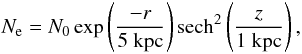 (1)where
N0 ≈ 3.2 × 10⁻⁴ cm-3 is derived from
the value for the CR electron density on Earth (Sun et al.
2008), and r and z are the radial and the
vertical coordinates in cylindrical galactocentric coordinates, respectively. This model
essentially assumes the same spatial density distribution for the CR electrons as for the
interstellar gas. At first order, this is what we would expect, because the higher the
interstellar gas density, the higher the star-formation rate, and therefore the higher the
supernova production, which gives a higher relativistic electron density. These cosmic
electrons lose energy (via synchrotron itself) on short distances of less than 1 kpc.
(1)where
N0 ≈ 3.2 × 10⁻⁴ cm-3 is derived from
the value for the CR electron density on Earth (Sun et al.
2008), and r and z are the radial and the
vertical coordinates in cylindrical galactocentric coordinates, respectively. This model
essentially assumes the same spatial density distribution for the CR electrons as for the
interstellar gas. At first order, this is what we would expect, because the higher the
interstellar gas density, the higher the star-formation rate, and therefore the higher the
supernova production, which gives a higher relativistic electron density. These cosmic
electrons lose energy (via synchrotron itself) on short distances of less than 1 kpc.
The value for N0 in Eq. (1) is very uncertain. This value is usually obtained by assuming that the CR electron spectrum can be described by a power-law with constant spectral index p = 3. However, observations in the last few years as well as numerical simulations (see Strong et al. 2007, and references therein) suggest that this assumption is not appropriate for the entire spectrum. Moreover, different observations show variations of the order of 50% (or even higher) for this quantity. Therefore, we expect that this uncertainty might introduce a bias in the recovered amplitude of the field strength for the different models, and will be taken into account as explained below.
In the following sub-sections we present the set of GMF models we investigate in this work, all of them taken from the literature. Most of these models have been proposed/constrained using the analysis of Faraday rotation of pulsars and EGRSs. Thus, it is also interesting to explore if these models are also able to describe the large-scale polarization pattern seen in WMAP 22 GHz maps. In total we investigate eight models describing the disk and halo fields, and one model conceived to describe the halo field. The disk models are: 1) axisymmetric (ASS), 2) axisymmetric with radial dependence of the strength (ASS(r)), 3) bisymmetric positive (BSS+), 4) bisymmetric negative (BSS−), 5) bisymmetric positive with radial dependence of the strength (BSS+(r)), 6) bisymmetric negative with radial dependence of the strength (BSS−(r)), 7) concentric circular rings (CCR) and 8) logarithmic spiral arms (LSA). Moreover we shall consider for the halo component the bi-toroidal (BT) model. Throughout this section, all coordinates (r,z) refer to cylindrical galactocentric coordinates.
2.1. Axisymmetric model
The axisymmetric model (see e.g. Vallee 1991;
Poezd et al. 1993) is one of the simplest
descriptions of the GMF. It is compatible with a non-primordial origin of the galactic
magnetism, based on the dynamo theory. There are several possible models of the family of
the axisymmetric distribution. The components for this model of GMF are given by
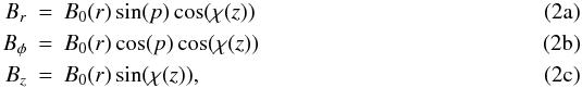 where
p is the pitch angle1, which is
considered to be constant; B0(r) is the field
strength (which in principle might be a function of the radial distance),
and χ(z) corresponds to a “tilt angle”. For our study,
we have adopted the following functional dependence
where
p is the pitch angle1, which is
considered to be constant; B0(r) is the field
strength (which in principle might be a function of the radial distance),
and χ(z) corresponds to a “tilt angle”. For our study,
we have adopted the following functional dependence
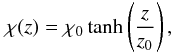 (3)where we use a value of
z0 = 1 kpc for the characteristic scale of variation in
the vertical direction.
(3)where we use a value of
z0 = 1 kpc for the characteristic scale of variation in
the vertical direction.
For the computations in this paper, we shall consider two cases for the radial dependence
of B0(r). The first case (hereafter ASS)
corresponds to
B0(r) = B0
(constant value). As a second case (hereafter ASS(r)), we consider a radial variation of
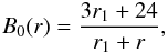
the type 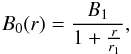 (4)where
r1 represents the characteristic scale at which
B0(r) decreases to half its value at the
galactic centre. This radial variation is based on a possible extension of the model by
Poezd et al. (1993). The expression has
appropriate asymptotic behaviors, in the sense that we obtain a finite value
when r is close to the galactic center (r → 0), and
asymptotically tends to ∝ 1/r when
r → ∞, as suggested in Battaner &
Florido (2007). We must note that in Eq. (4), B1 and r1 are not
independent, provided that we fix the value of the GMF strength in the solar neighborhood.
For example, using R0 = 8 kpc for the Sun galactocentric
distance, and B⊙ = 3 μG for the magnetic
field strength in the solar neighborhood, we can re-write Eq. (4) in terms of a single free-parameter as
(4)where
r1 represents the characteristic scale at which
B0(r) decreases to half its value at the
galactic centre. This radial variation is based on a possible extension of the model by
Poezd et al. (1993). The expression has
appropriate asymptotic behaviors, in the sense that we obtain a finite value
when r is close to the galactic center (r → 0), and
asymptotically tends to ∝ 1/r when
r → ∞, as suggested in Battaner &
Florido (2007). We must note that in Eq. (4), B1 and r1 are not
independent, provided that we fix the value of the GMF strength in the solar neighborhood.
For example, using R0 = 8 kpc for the Sun galactocentric
distance, and B⊙ = 3 μG for the magnetic
field strength in the solar neighborhood, we can re-write Eq. (4) in terms of a single free-parameter as
 (5)where
r is given in kpc and
B0(r) in μG.
(5)where
r is given in kpc and
B0(r) in μG.
Summarizing, a particular ASS model is fully described once these three parameters are given: [B0,p,χ0] , while in the ASS(r) model, one would in principle require four parameters. However, for the ASS(r) family of models, we will use the constraint given in Eq. (5), which in practice means that we will only have three free parameters to represent a certain model: [r1,p,χ0] .
The typical range of variation of the p values found in the literature for the ASS model of the disk (see Vallee 1991) is shown in Table 1. In general, different pitch angle and field strength values are derived for the different spiral arms of the Galaxy.
2.2. Bisymmetric model
This model is compatible with a primordial origin of the cosmic magnetism. It could
explain the reversals of the magnetic field derived from observations of RM of pulsars
(e.g. Han & Qiao 1994; Han 2001; Han et al.
2006). The three components for this model are given by 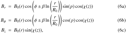 where
B0(r) is the field strength;
β = 1/tan(p), with
p the pitch angle; R0 is the distance
Sun-Galactic center (≈8 kpc); and finally χ(z) is the
tilt angle, which we assume is also given by Eq. (3). Note that in Eq. (6) we are
considering two possible families of bisymmetric models, which correspond to the positive
(negative) sign inside the big parenthesis for
Br
and Bφ. In this way, we are considering
the two conventions that are found in the literature. “Positive” bisymmetric models
(hereafter BSS+) are defined with the same convention to recover the model
proposed by Han & Qiao (1994), while
“negative” bisymmetric models (hereafter BSS−) use the same sign convention of
Jansson et al. (2009). Note that for
BSS− the spiral has the opposite sign for the magnetic direction.
where
B0(r) is the field strength;
β = 1/tan(p), with
p the pitch angle; R0 is the distance
Sun-Galactic center (≈8 kpc); and finally χ(z) is the
tilt angle, which we assume is also given by Eq. (3). Note that in Eq. (6) we are
considering two possible families of bisymmetric models, which correspond to the positive
(negative) sign inside the big parenthesis for
Br
and Bφ. In this way, we are considering
the two conventions that are found in the literature. “Positive” bisymmetric models
(hereafter BSS+) are defined with the same convention to recover the model
proposed by Han & Qiao (1994), while
“negative” bisymmetric models (hereafter BSS−) use the same sign convention of
Jansson et al. (2009). Note that for
BSS− the spiral has the opposite sign for the magnetic direction.
As in the previous case, we consider two sub-families of models. The first one, noted as BSS±, corresponds to constant strength of the magnetic field. In this case, a model is completely defined by giving three parameters: [B0,p,χ0] . The second family, noted as BSS±(r), includes a radial variation of the field strength according to Eq. (4). For this case, we again fix the field strength to the value in the Solar neighborhood (Eq. (5)), so a model is specified by giving three parameters: [r1,p,χ0] .
Typical parameter values for the disk model found in the literature, after conversion to our convention for the sign of the pitch angle, are p = (8.2 ± 0.5)°, B0 = 1.4 μG and Bglobal = (1.8 ± 0.3) μG (Han & Qiao 1994); p = 14° and B0 = 1 μG (Simard-Normandin & Kronberg 1980); and p = 11° and B0 = (2.1 ± 0.3) μG (Han et al. 2006).
2.3. Concentric circular ring (CCR) model
This model was proposed by Rand & Kulkarni
(1989) to fit the RM of their pulsars catalog, with the aim of providing a way to
take into account reversals of the magnetic field at different radii. In their original
expressions, they do not consider a vertical component for the magnetic field (i.e.
Bz = 0). Here, we shall extend the
equations for this model presented in Indrani &
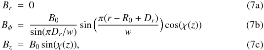
Deshpande (1999) to account for a vertical dependence in the following way
 where
w is the space between reversals;
Dr is the distance to the first reversal;
B0 is the field strength, and finally
χ(z) is given by Eq. (3). All distances (w and
Dr) are given in kiloparsecs. Note that
we introduce an additional factor
sin(πDr/w)
in the definition of Bφ, so
B0 still preserves the meaning of the magnetic field
strength in the solar neighborhood.
where
w is the space between reversals;
Dr is the distance to the first reversal;
B0 is the field strength, and finally
χ(z) is given by Eq. (3). All distances (w and
Dr) are given in kiloparsecs. Note that
we introduce an additional factor
sin(πDr/w)
in the definition of Bφ, so
B0 still preserves the meaning of the magnetic field
strength in the solar neighborhood.
In our analyses we did not consider any radial dependence of the field strength, so for the CCR model the parameter space is defined by [Dr,w,B0,χ0] .
The best-fit values obtained by Rand & Kulkarni (1989) for the disk component were Dr = (0.6 ± 0.08) kpc , w = (3.1 ± 0.08) kpc and B0 = (1.6 ± 0.2) μG.
2.4. Logarithmic spiral arms (LSA) model
This model was used by Page et al. (2007) to
describe the distribution of the large-scale pattern of the polarization angle in the
22 GHz WMAP 3-year data. The equations which describe the field are 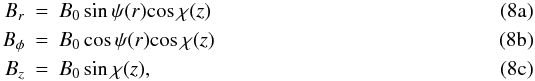 where
where
 and
and
 Note that the LSA model
is essentially an axisymmetric model in which the pitch angle is not constant, because
magnetic field lines are logarithmic spirals. According to our definition of pitch angle
for the ASS model, ψ(r) would play the role of pitch
angle, in which we would have a constant part, ψ0, and a
characteristic amplitude for the logarithmic dependence of the arms,
ψ1. Following Page et al.
(2007), B0 is assumed constant with a value of
3 μG.
Note that the LSA model
is essentially an axisymmetric model in which the pitch angle is not constant, because
magnetic field lines are logarithmic spirals. According to our definition of pitch angle
for the ASS model, ψ(r) would play the role of pitch
angle, in which we would have a constant part, ψ0, and a
characteristic amplitude for the logarithmic dependence of the arms,
ψ1. Following Page et al.
(2007), B0 is assumed constant with a value of
3 μG.
Thus, the parameter space is defined by [ψ0,ψ1,χ0] . The proposed values for the different parameters are [ψ0,ψ1,χ0] = [27°,0.9°,25°] (see Page et al. 2007, and also the erratum available at the LAMBDA web site2).
2.5. Bi-toroidal (BT) model (halo model)
Some authors have found hints of a halo or thick disk field component with opposite directions in both hemispheres. For example, Han & Wielebinski (2002) and Prouza & Šmída (2003) detected it with maximum strengths at a large height of 1.5 kpc at both sides above and below the plane, with maximum strengths of approximately 1 μG. Sun et al. (2008) give a more complete description of this double torus, with the height of maximum strength again at 1.5 kpc, but its maximum is much stronger (around 10 μG).
Following this scenario, we propose a possible configuration for the components of the
magnetic field which do contain a different sign in both hemispheres, and it is given by
 where
σ1 and σ2 are two constants
(measured in kpc) which encode the characteristic scales of variation of the field with
the vertical distance, and do take into account in a simplified way the change in the
sign. For our computations, we fix the Bz
value to be 0.2 μG (Han & Qiao
1994), and we only consider the case of a radial variation of
B0(r) given by Eq. (5). Thus, the parameter space for this model is
specified by
[r1,σ1,σ2] .
where
σ1 and σ2 are two constants
(measured in kpc) which encode the characteristic scales of variation of the field with
the vertical distance, and do take into account in a simplified way the change in the
sign. For our computations, we fix the Bz
value to be 0.2 μG (Han & Qiao
1994), and we only consider the case of a radial variation of
B0(r) given by Eq. (5). Thus, the parameter space for this model is
specified by
[r1,σ1,σ2] .
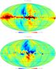 |
Fig. 1 Observed Stokes Q (top) and U (bottom) maps at 22 GHz from WMAP5 data. The maps are shown in a Mollweide projection of HEALPix in Galactic coordinates. The center of the map corresponds to (l,b) = (0°,0°), and the graticule increases with Δl = Δb = 45°. The maps are degraded to nside = 16 to enhance the large scale pattern. Units are mK (thermodynamic). |
3. Methodology
In order to obtain constraints on the different parameters for each one of the models described above, we performed a systematic comparison of the predicted polarized intensity due to synchrotron emission with the observed map at 22 GHz by WMAP satellite. Here, we describe the relevant details of the dataset, the numerical procedure to compute the synchrotron maps for a certain GMF model, and the model selection criterion that we adopted for our analyses.
3.1. Description of the K-band WMAP5 data
The analysis of this paper is based on a comparison with the K-band (equivalent to 22 GHz) polarization map obtained by the WMAP satellite after five years of operation (Hinshaw et al. 2009). This map is publicly available in the LAMBDA website3, and it is given in HEALPix4 format (Górski et al. 2005).
Figure 1 shows the all-sky Stokes Q and U maps at 22 GHz, degrading the resolution to enhance the large-scale pattern, using an nside = 16 pixelization (which corresponds to a pixel size of 3.66°). For all the computations in this paper, we will use these degraded maps as the input data. As shown by the WMAP team (Page et al. 2007), at this frequency (22 GHz) the large-scale pattern observed in polarization is completely dominated by the galactic contribution, and the CMB component is sub-dominant. Thus, we can safely neglect the contribution of the CMB to the polarization map in our analyses.
From these two observables (Stokes Q and U parameters),
one can obtain the map of the direction of the polarization angle (hereafter PA) as
 (10)where
 is the direction of the line of sight. Note
that we include in our definition the π/2 factor, so
Eq. (10) represents the angle of the
magnetic field, and takes values in the [ 0,π ] region. Note that the
polarization convention adopted here is the one described in HEALPix, labelled as
COSMO, which differs from the usual IAU convention in a minus sign for Stokes
U parameter. In addition, the WMAP definition of Stokes parameters
includes an additional 1/2 factor with respect to the definition used
by Chandrasekhar (1960), which will be the one
adopted here. All these quantities (U, Q and PA) are
defined in a galactic (heliocentric) coordinate system. This has to be taken into account
when comparing the observed maps with the models. Figure 2 shows the observed direction of the PA at the same 3.66°
(nside = 16) resolution.
is the direction of the line of sight. Note
that we include in our definition the π/2 factor, so
Eq. (10) represents the angle of the
magnetic field, and takes values in the [ 0,π ] region. Note that the
polarization convention adopted here is the one described in HEALPix, labelled as
COSMO, which differs from the usual IAU convention in a minus sign for Stokes
U parameter. In addition, the WMAP definition of Stokes parameters
includes an additional 1/2 factor with respect to the definition used
by Chandrasekhar (1960), which will be the one
adopted here. All these quantities (U, Q and PA) are
defined in a galactic (heliocentric) coordinate system. This has to be taken into account
when comparing the observed maps with the models. Figure 2 shows the observed direction of the PA at the same 3.66°
(nside = 16) resolution.
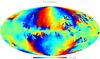 |
Fig. 2 Observed direction of the polarization angle (PA) at 22 GHz, obtained from the two maps shown in Fig. 1. The PA is defined here as the local direction of the magnetic field (see Eq. (10)). Units are degrees. |
3.1.1. Noise maps
In order to perform the model selection, we also need to estimate the noise maps associated to the data. It is important to note that those noise maps should account for the covariances introduced by all components which are present in the observed data but are not included in the theoretical model. In particular, it should account for the instrumental noise component and for the random component of the GMF, which are not included in our theoretical model. The first one could be easily estimated based on the information provided by the WMAP team about instrument sensitivity and the overall integration time that the satellite has spent on each particular pixel. However, this would not account for the second part of the covariance. Thus, in order to model all the different contributions to the covariance, we follow a different procedure, which makes use of the fact that the original WMAP-K band maps have a much better angular resolution than the pixel size that is finally adopted in our analyses.
Noise maps for Q and U.
In this paper we probed three different methods to characterize the noise maps associated to Q and U. In addition to the pure instrumental noise, all these three methods attempt to estimate the contribution to the total covariance matrix of the residual astrophysical components which are not included in our model (for example, the random component of the magnetic field, or the variance introduced by point-to-point variations of the mean level of the galactic emission). All methods produce a noise map at nside = 16 resolution, which provides a pixel size of ~3.66°. The three methods to obtain the σQ map (or equivalently, the σU), are
-
Method 1. This corresponds to the same procedure asdescribed in Jansson etal. (2008). We start from the observed WMAPStokes-Q map at full resolution (nside = 512), degrading it to ~0.92° pixel resolution (nside = 64). For a given pixel i within our nside = 16 pixelization scheme, we obtain the associated noise σQ(i) by computing the square root of the variance of the ~0.92° pixels inside a radius of 2° from the center of our pixel i.
-
Method 2. We start from the observed Q-map at nside = 512, and we convolve it with a Gaussian of FWHM = 1°. For a given pixel i within our nside = 16 pixelization scheme, the associated noise σQ(i) is computed as the square root of the variance in each pixel of the smoothed map within a radius of 2° from the center of our pixel i.
-
Method 3. We start from the observed WMAP Stokes-Q map degraded at nside = 16. For each pixel i, the noise σQ(i) is computed by obtaining the square root of the variance inside a circle of radius r ~ 7.4° (i.e. twice the pixel radius). This method produces an unbiased estimate of the noise map in the case of uncorrelated noise, provided that the scale of variation of the noise map is larger than 7.4°.
Each one of these three methods produces different results for the noise map in certain areas, specially those dominated by galactic features. In turn, these differences imply significant changes in the goodness-of-fit statistic (up to a factor of 2−3 in some cases).
In general, we find that the larger noise amplitudes are obtained with method 1, while the smaller amplitudes are obtained with method 2.
Thus, and as a conservative approach, we decided to present the computations of this paper using the method 3.
The implications of this uncertainty in the determination of the noise maps are discussed in Sect. 5.
Noise maps for the Stokes Q and U parameters, obtained with method 3, are shown in Fig. 3. These maps have been used to obtain the final results presented in Tables 3 and 4.
Noise maps for PA.
Once these two noise maps (σQ and σU) have been obtained, one can in principle obtain the noise map associated to the PA (σγ) from them. However, there is an important point here. Equation (10), which defines the PA, is not linear in Q and U. This implies that the variance map for the PA will depend on the particular model which is used to compute the average value; or in other words, the noise map for PA will depend not only on σQ and σU, but also on Q and U themselves. Therefore, when doing the model selection, the noise map for PA will also be a function of the model.
To illustrate this, we compute here the noise map for PA, using as reference model the observed WMAP-K map. We use here a Monte Carlo method, drawing Nsim realizations of pairs of (Q,U) maps, with mean equal to the observed (Q,U) maps, and variance given by σQ and σU, as computed in previous step. We have checked that using Nsim = 5000 noise realizations is enough to get convergence on the σγ map at the per cent level. Figure 3 also shows the noise map for the PA, obtained for this particular case.
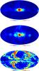 |
Fig. 3 Noise maps for the WMAP5 datasets presented in Figs. 1 and 2. They show the Stokes Q (top), Stokes U (middle) and position angle (PA, bottom) maps. Units for Stokes Q and U maps are mK. Units for the PA map are degrees. The noise map for PA has been computed as fluctuations around the observed WMAP5 K-band map. |
3.2. Producing the synchrotron polarized emission for a given magnetic field model
To obtain the predicted polarized synchrotron emission for any of the Galactic magnetic field models described above, we have developed a code which only includes the relevant physics, and it is optimized in terms of computational time with the aim of efficiently performing all the computations. The code works directly within the HEALPix pixelization scheme, and obtains the predictions for the synchrotron emission directly at the resolution level that we have chosen (i.e. nside = 16). As discussed above, this resolution is enough as long as we are interested in the large-scale pattern of the Galactic emission.
In general, assuming that the cosmic ray spectrum is a power-law distribution of spectral
index p, we can predict the Stokes Q
and U parameters that characterize the polarization of the synchrotron
emission at a certain frequency by computing the emissivity (energy per unit time per unit
volume per frequency per solid angle) in the two orthogonal directions, parallel and
perpendicular to the projection of the magnetic field on the plane of the sky. Following
Rybicki & Lightman (1986), we have
![Mathematical equation: \begin{eqnarray} \nonumber &&\epsilon_{\perp}(\nu) = N(r,z) \frac{\sqrt{3}e^{3}}{8\pi m c^{2}} \left( \frac{4 \pi mc}{3e} \right)^{\frac{1-p}{2}} \nu^{\frac{1-p}{2}} (B\sin\alpha)^{\frac{p+1}{2}} \qquad \\ & &\qquad\quad \times \Gamma\left ( \frac{p}{4} - \frac{1}{12} \right ) \left [ \frac{2^{\frac{p+1}{2}}}{p+1} \Gamma\left ( \frac{p}{4} + \frac{19}{12} \right ) + 2^{\frac{p-3}{2}} \Gamma\left ( \frac{p}{4} + \frac{7}{12} \right ) \right ] \label{eq:power_perp} \end{eqnarray}](/articles/aa/full_html/2010/14/aa12733-09/aa12733-09-eq115.png) (11)
(11)
![Mathematical equation: \begin{eqnarray} \nonumber &&\epsilon_{||}(\nu) = N(r,z) \frac{\sqrt{3}e^{3}}{8\pi m c^{2}} \left( \frac{4 \pi mc}{3e} \right)^{\frac{1-p}{2}} \nu^{\frac{1-p}{2}} (B\sin\alpha)^{\frac{p+1}{2}} \\ & & \qquad\quad\times\Gamma\left ( \frac{p}{4} - \frac{1}{12} \right ) \left [ \frac{2^{\frac{p+1}{2}}}{p+1} \Gamma\left ( \frac{p}{4} + \frac{19}{12} \right ) - 2^{\frac{p-3}{2}} \Gamma\left ( \frac{p}{4} + \frac{7}{12} \right ) \right ], \label{eq:power_paral} \end{eqnarray}](/articles/aa/full_html/2010/14/aa12733-09/aa12733-09-eq116.png) (12)where
B is the magnetic field, ν is the frequency,
p is the spectral index, and e and m
are the electron charge and mass, respectively. The function
N(r,z) represents the electron number density at the
corresponding position (r,z) in the Galaxy, and it is obtained from
Eq. (1). From these two equations, the
polarized intensity at a given frequency is obtained by integrating the emissivity along
the line of sight
(12)where
B is the magnetic field, ν is the frequency,
p is the spectral index, and e and m
are the electron charge and mass, respectively. The function
N(r,z) represents the electron number density at the
corresponding position (r,z) in the Galaxy, and it is obtained from
Eq. (1). From these two equations, the
polarized intensity at a given frequency is obtained by integrating the emissivity along
the line of sight ![Mathematical equation: \begin{equation} \label{intensity} I_{\nu}(z,\hat{n}) \equiv (Q_{\nu} - iU_{\nu})= \int{[\epsilon_{\perp}(\nu,z,\hat{n})-\epsilon_{||}(\nu,z,\hat{n})]{\rm e}^{-i 2\change{\gamma}(z,\hat{n})}{\rm d}z}, \end{equation}](/articles/aa/full_html/2010/14/aa12733-09/aa12733-09-eq123.png) (13)where we have set the
coordinate system in a way that the z-axis represents the line-of-sight
direction, and the other two directions are contained in the plane on the sky, with the
y-axis pointing east and x-axis pointing south (i.e.
HEALPix coordinate convention, as explained in Sect. 3.1). With these definitions, the Stokes Q and
U parameters are given by
(13)where we have set the
coordinate system in a way that the z-axis represents the line-of-sight
direction, and the other two directions are contained in the plane on the sky, with the
y-axis pointing east and x-axis pointing south (i.e.
HEALPix coordinate convention, as explained in Sect. 3.1). With these definitions, the Stokes Q and
U parameters are given by ![Mathematical equation: \begin{subequations} \label{eq:q-u-theo} \begin{eqnarray} \label{eq:q} Q_{\nu} &= \int{[\epsilon_{\perp}(\nu,z,\hat{n})-\epsilon_{||}(\nu,z,\hat{n})]\cos(2\gamma){\rm d}z}\\ \label{eq:u} U_{\nu} &= \int{[\epsilon_{\perp}(\nu,z,\hat{n})-\epsilon_{||}(\nu,z,\hat{n})]\sin(2\gamma){\rm d}z}, \end{eqnarray} \end{subequations}](/articles/aa/full_html/2010/14/aa12733-09/aa12733-09-eq126.png) By
assuming a spectral index p = 3, we obtain the
simulated Q and U components along the line of sight
(z-axis) by numerical integration
By
assuming a spectral index p = 3, we obtain the
simulated Q and U components along the line of sight
(z-axis) by numerical integration ![Mathematical equation: \begin{subequations} \label{eq:q-u-sim} \begin{eqnarray} \label{qsim} Q_{\nu}(\hat{n}) &= K_{Q}(\nu)\int_{\rm LOS}{N_{\rm e}(\hat{n})[B_{x}^{2} - B_{y}^{2}] {\rm d}z} \\ \label{usim} U_{\nu}(\hat{n}) &= -K_{U}(\nu)\int_{\rm LOS}{ N_{\rm e}(\hat{n}) 2B_{x} B_{y} {\rm d}z}, \end{eqnarray} \end{subequations}](/articles/aa/full_html/2010/14/aa12733-09/aa12733-09-eq128.png) where
we explicitly introduce a minus sign in the equation for the U component,
in order to convert from the IAU convention for the polarization to the HEALPix
convention, which is used in the WMAP maps. The
KU(ν) and
KQ(ν) constants also
include the conversion factors between brightness and temperature. At 22 GHz, we can
safely use the Rayleigh-Jeans approximation. Substituting the numerical values, we obtain
KQ(ν) = 1.41 × 10¹¹ mK cm3 (μG)-2 kpc-1,
and
KU(ν) = 1.25 × 10¹¹ mK cm3 (μG)-2 kpc-1.
The simulated PA map is derived from these two Eq. (15) as
where
we explicitly introduce a minus sign in the equation for the U component,
in order to convert from the IAU convention for the polarization to the HEALPix
convention, which is used in the WMAP maps. The
KU(ν) and
KQ(ν) constants also
include the conversion factors between brightness and temperature. At 22 GHz, we can
safely use the Rayleigh-Jeans approximation. Substituting the numerical values, we obtain
KQ(ν) = 1.41 × 10¹¹ mK cm3 (μG)-2 kpc-1,
and
KU(ν) = 1.25 × 10¹¹ mK cm3 (μG)-2 kpc-1.
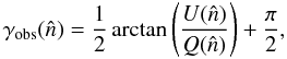
The simulated PA map is derived from these two Eq. (15) as ![Mathematical equation: \begin{equation} \label{gammasim} \gamma(\hat{n}) = 0.5 \arctan \left( \frac{-K_{U}(\nu)\int_{\rm LOS}{ N_{\rm e}(\hat{n}) 2B_{x} B_{y} {\rm d}z}}{K_{Q}(\nu)\int_{\rm LOS}{N_{\rm e}(\hat{n})[B_{x}^{2} - B_{y}^{2}] {\rm d}z}} \right) + \frac{\pi}{2}, \end{equation}](/articles/aa/full_html/2010/14/aa12733-09/aa12733-09-eq136.png) (16)where
Bx and
By represent in our coordinate system the
two components of the magnetic field which are perpendicular to the line of sight.
(16)where
Bx and
By represent in our coordinate system the
two components of the magnetic field which are perpendicular to the line of sight.
Finally, when predicting the expected synchrotron emission for a particular model, we have included an additional restriction on the line-of-sight integration by excluding those points whose galactocentric radial coordinate rG is smaller than 3 kpc or larger than 20 kpc. The first restriction excludes the inner region of the Galaxy, where large deviations from the regular pattern are expected (La Rosa et al. 2006), while the second one introduces a radial cut-off. In any case, we have checked that the results are robust against changes in these numbers.
3.3. Exploration of the parameter space
As described in Sect. 2, for each one of the families of GMF models we have a set of parameters which define each particular model. Given that in all cases the dimension of the parameter space is small (there are, at the most, four parameters describing a particular model), we decided to carry out the exploration of the parameter space using a grid-based approach. For higher dimensions, a Monte Carlo method would be more appropriate.
For each one of the different GMF models we constructed three different grids of models, which we label as “literature”, “blind” and “non-blind”. The first one is centered around the average values which are found in the literature for each one of the different parameters. The second one spans the maximum range which is reasonably expected for each particular parameter. Finally, the third one is built a-posteriori, once the model selection has been performed on the previous grid, by centering the new grid around the best-fit parameters for each case. Table 1 summarizes all the relevant parameters for each one of these three grids. In total we computed more than one million models (290 000 for the blind grid, 970 000 for the non-blind, and 51 000 for the literature) for all the different GMF models described in Sect. 2. Each one of those models corresponds to a set of three maps (Q, U and PA) of the expected synchrotron polarized emission of the sky at 22 GHz.
To give an indication, the average execution time in a standard desktop computer for the computation of a particular model requires ≲ 4 s of CPU time. Thus, the total CPU time for the construction of all the grids is around 1500 CPU hours.
Exploration of the parameter space.
3.4. Model selection and parameter estimation for each GMF model
Once we explored the parameter space with these three grids, we derived the best-fit parameters for each one of the GMF models using a Bayesian approach. To this end, we have to both compute the likelihood function (ℒ), and to provide an expression for the priors. Once we obtained the best-fit parameters for each GMF model, different models will be compared in terms of the reduced-χ2 statistic.
3.4.1. Likelihood function
In general, we may assume that the likelihood function is defined as a multivariate
Gaussian when it is written in terms of the observables, i.e.
 (17)If we assume that the
correlations between the different pixels are negligible, we have
(17)If we assume that the
correlations between the different pixels are negligible, we have 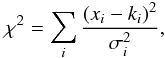 (18)where
xi represents the observational data,
ki the simulated data and
(18)where
xi represents the observational data,
ki the simulated data and
 , the associated noise
covariance. In our case, we performed two different evaluations of the likelihood:
, the associated noise
covariance. In our case, we performed two different evaluations of the likelihood:
-
the first one corresponds to a direct comparison of Stokes Q and U parameters. In this case, we have i = 1,...,2Npix, and xi = Qi for i = 1,Npix; and xi = Ui − Npix for i = Npix + 1,...,2Npix. This case will be noted as
 ;
; -
the second case corresponds to the comparison of PA, so now we have i = 1,...,Npix, and xi = γi. Note that in this case, σi will depend on ki, and thus the PA noise map needs to be computed for each particular model. This case will be noted as
 , and will be used for
comparison with the results of the previous case.
, and will be used for
comparison with the results of the previous case.
Once these two functions ( and
) are evaluated in all the
data-points of the different grids, the posterior distributions are obtained, and then
marginalized5 over all the unwanted parameters.
At the end, we end up with marginal probability distribution functions for each one of
the parameters. From these, confidence intervals are derived as the 0.16, 0.5 and
0.84 points of the cumulative probability distribution function. Thus, our parameter
estimate is the median of the marginalized posterior probability distribution function,
and the confidence interval encompasses 68 per cent of the probability.
3.4.2. Priors
For the analyses in this paper, we have not introduced prior information on the parameter values describing any of the models. This is equivalent to say that we have implicitly adopted a top-hat prior in all the parameters, where the top-hat function is defined by the parameter ranges presented in Table 1. Thus, in all cases, the evaluation of the posterior would reduce to the computation of the likelihood function (ℒ).
However, for the case of (Q,U) analysis, we slightly modified the
standard analysis in the following way. As discussed in Sect. 2, the amplitude of the CR electron spectrum in the solar neighborhood
is highly uncertain. This will in turn imply a large uncertainty in the recovered
strength for the magnetic field, and moreover, it might produce a bias on the recovered
GMF amplitude. To account for this additional degree of uncertainty (at least at first
order), we have introduced an additional parameter ϵ, which multiplies
to both the predicted Q and U maps for a given GMF
model. Note that this parameter has no impact on PA. If the CR electron density were
entirely correct, we would have ϵ = 1. If there is an uncertainty in
this parameter due to the modeling of the CR distribution, we account for it by
introducing a Gaussian prior for this additional parameter 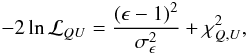 (19)and we marginalize
over it. Given the existing uncertainty on the CR electron density, we have chosen a
conservative value of σϵ = 0.8. The
marginalization over this additional parameter, ϵ, can be done
analytically, yielding
(19)and we marginalize
over it. Given the existing uncertainty on the CR electron density, we have chosen a
conservative value of σϵ = 0.8. The
marginalization over this additional parameter, ϵ, can be done
analytically, yielding 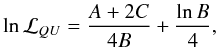 (20)where
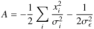 (21)
(21) (22)
(22) (23)Note that this scheme
is completely equivalent to the marginalization over calibration uncertainties which is
also adopted in CMB experiments (see e.g. Bridle et al.
2002).
(23)Note that this scheme
is completely equivalent to the marginalization over calibration uncertainties which is
also adopted in CMB experiments (see e.g. Bridle et al.
2002).
3.5. Masks
Nearby structures in the Galaxy (e.g. supernova remnants) might distort the regular pattern of the GMF as seen in the synchrotron polarized emission, thus biasing the determination of some parameters of the GMF model. To probe the robustness of the estimates as a function of the region which is used for the fit, we have considered different masks to constrain the global, halo and disk components of the GMF. In all cases, we exclude the galactic center region defined as the region in which the line of sight crosses a region with radius 3 kpc in cylindrical coordinates, that is not taken into account in our integration scheme. To constrain the global component we considered two masks, listed in decreasing order of covered sky fraction:
-
Mask 1. It corresponds to the Galactic center region.
-
Mask 2. It combines mask 1 with the well-known local regions with a strong polarized intensity that could be interpreted as part of the polarized intensity produced by the regular GMF. Here we considered the four “loops” described in Berkhuijsen et al. (1971), and we added the polarization mask from WMAP team, which includes a better masking of the North Galactic spur region and several other small objects (e.g. LMC).
To constrain the halo component we exclude the following regions:
-
Mask 3. It excludes the disk defined as the emission contains in |b| < 10°.
-
Mask 4. It excludes the emission of the disk (mask 3) and the “loops” defined in mask 2.
For completeness, we also considered two masks to constrain the field pattern in the disk. They are
-
Mask 5. It excludes the halo region defined as the emissionobtained for |b| > 10°.
-
Mask 6. It excludes the halo and the “loops” described in Berkhuijsen et al. (1971).
In Fig. 4 we show all regions which have been described in this subsection. Figure 5 shows the polarization mask used by the WMAP team6. Table 2 presents the detailed information about the sky coverage of each one of these masks. It also indicates the number of available pixels for the analysis (i.e. number of terms in the summation in Eq. (18). This quantity is relevant in order to compute the reduced-χ2 for the best-fit models. As a reference, note that in this pixelization (nside = 16), a whole-sky map contains 3072 pixels. Therefore, we would have in this case Npix(QU) = 6144.
Note that even if we use these masks to eliminate the effects of the random local spurs, other undetected random local features could be a source of errors in our large-scale models and these errors are difficult to quantify. But our spur masks probably eliminate the major contribution of local features.
Galactic masks used in the analyses.
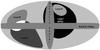 |
Fig. 4 Regions used for the definition of the six masks adopted for the analyses (see text for details). |
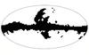 |
Fig. 5 Mask for the galactic polarized emission used by the WMAP team. |
Best-fit parameters for the global and halo component of the GMF model (masks 1, 2, 3, and 4), based on the analysis of the Stokes Q and U parameters.
4. Results and discussion
For each one of the masks described in Table 2 and for each one of the GMF models presented in Sect. 2, we evaluate the posterior distribution in each one of the three grids, and marginalizing over the relevant parameters, we obtain the corresponding confidence regions. Our default analysis uses the Q − U maps, and the noise maps obtained with method 3 in Sect. 3.1.1. The results are summarized in Tables 3 and 4.
In order to evaluate which model better reproduces the data, we used as a goodness-of-fit the reduced-χ2 statistic, which is obtained as the ratio of the the minimum value for χ2(≡ −2lnℒQU) to the number of degrees of freedom (hereafter d.o.f.). The number of dof is obtained as Npix − M, being Npix the number of terms in Eq. (18), and M the number of parameters for the considered GMF model. The last two columns in each table present the values for the minimum χ2, and the reduced-χ2.
4.1. The magnetic field in the Galactic halo
The results for the halo field are summarized in Table 3.
Our reference computation corresponds to the case labelled as mask 4, in which we exclude the emission of the disk, the “loops” (including the polarization mask provided by the WMAP team), and the galactic center region (which is not accounted for in our analysis). For this reference case, the model with the minimum reduced-χ2 is the ASS(r), although the other two axisymmetric models (LSA and ASS) provide approximately the same goodness-of-fit. Thus, the large-scale 22 GHz polarized synchrotron emission seems to be more compatible with some type of axisymmetry, a conclusion also reached by Page et al. (2007), and also compatible with the results shown by Sun et al. (2008). For illustration, Fig. 6 shows the field pattern of the best-fit ASS(r) model at z = 4 kpc; Fig. 7 shows the marginalized one-dimensional posteriors distributions for the parameters of this model; and Fig. 8 shows the predicted Stokes Q and U and PA maps for the same best-fit model. We now discuss each one of the relevant parameters separately.
Radial scale.
For this ASS(r) model, the derived constraint on r1 is
<2.5 kpc (95% confidence level). This parameter essentially
controls the distance at which the magnetic field is no longer constant and begins to
decrease proportional to r-1 (see Eq. (5)). The obtained value is indeed very small
compared with the radial scale of the electron density or any other scale distance in
our galaxy, suggesting that the data require an important variation of the field in the
inner part of the halo, probably due to the presence of stronger magnetic fields at the
galactic center (see e.g. Roy et al. 2008).
Indeed, in the literature, the halo model proposed in Prouza & Šmída (2003) requires also a small radial scale of
r1 = 4 kpc, where the radial dependence is
∝  in that case.
Field strength.
For the ASS(r), we adopted a fixed value for the magnetic field strength of
B0 = 3 μG at the solar neighborhood. The
original LSA model proposed by Page et al. (2007)
also assumed this fixed value. However, it was considered as a free parameter for the
ASS model, and was found to agree with that value ( μG).
μG).
Pitch angle.
The pitch angle was considered in the ASS(r) and ASS models as a constant free parameter. In both cases, we consistently obtain a value between 24° and 26° respectively. For the LSA model, it is considered as a radial function with a logarithmic dependence, and in this case the derived pitch angle at the solar neighborhood is again ≈26°, a value which is consistent with that given by Page et al. (2007) of p = 27°. As discussed below, these values are higher than the typical pitch angles obtained for the disk field.
Tilt angle.
This parameter controls the vertical structure of the field. The derived tilt angle in all the axysimmetric models is of the order of 30°, which implies a vertical component close to 1 μG at z = 1 kpc. This vertical field component could be identified as the poloidal component corresponding to the dipole field responsible of the mG vertical component at the very center (Han & Qiao 1994). It could correspond as well to the vertical component of the cluster field diffused into the disk by turbulent magnetic diffusion (e.g. Battaner & Florido 2000), in this case to the Local Group field.
Other models.
Table 3 shows a good consistency between the three axisymmetric models. The rest of the families considered here provide slightly worse reduced-χ2 values, although none can be clearly rejected. In general, the two families of bisymmetric models provide a slightly poorer goodness-of-fit. The derived radial scales, field strengths and pitch angles are in general similar to those found for the axisymmetric models. However, the tilt values (χ0) are considerably lower, and in some cases negligible. This could be due to a compensation produced by the inherent reversals of the fields for a given direction in a bisymmetric configuration.
The two remaining models (CCR and BT) produce the poorer fits (χ2 = 2.1), but again they cannot be rejected. With regard to these values, the CCR points to the existence of a reversal at r ~ 3 kpc from the galactic center. The bi-toroidal model has been suggested as a possible explanation for the halo double torus that it is interpreted by Han et al. (1997, 1999) and Han (2009) as a consequence of an α−Ω effect. Another possibility is that the aforementioned vertical field diffused from the galaxy cluster could be twisted by differential rotation in the vertical direction, producing toroidal fields above and below the plane with opposite directions in both hemispheres (e.g. Battaner & Florido 2000).
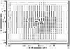 |
Fig. 6 Large-scale pattern of the ASS(r) model at z = 4 kpc. This model provides the best fit for the halo field. |
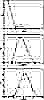 |
Fig. 7 One dimensional (marginalized) posterior distribution functions for the parameters of ASS(r) halo model (top: r1, middle: p and bottom: χ0) when mask 4 is considered in the Stokes Q and U analysis. |
Effect of the loops and the disk emission on the determination of the halo field.
As described in Sect. 3.5, nearby structures in the Galaxy might introduce biases on the recovered parameters of a given GMF model. Moreover, the emission of the disk could contaminate the halo field as discussed in Sect. 1. If the disk emission is not excluded by the mask, we could constrain the global component of the GMF and quantify the impact of the disk emission on the parameters describing halo field. The corresponding results are also shown in Table 3.
The influence of disk emission can be seen by comparing the results from masks 2 and 4. In both cases, the best-fits are obtained for axisymmetric models but when disk emission is not masked out, the reduced-χ2 becomes slightly poorer. In general, the pitch and tilt angles and the field strength remain unchanged, with the important exception of the radial scale factor for ASS(r) and BSS±(r) models. The inclusion of the disk emission in the analysis drastically increases this radial scale, probably because as shown below, the disk does not require strong radial variations.
Finally, we can also evaluate the impact of the loops on the fit by comparing the results of masks 3 and 4, or 1 and 2. The basic conclusion in this case is that including the loop regions in the analysis do not significantly bias the results (even for the radial scale parameter), but the quality of the fits get worse in all cases.
4.2. The magnetic field in the disk
For completeness, we also used two masks (5 and 6) to study the magnetic field in the Galactic plane by masking the halo emission. Table 4 summarizes the constraints on the different parameters for this case. The reference mask now is number 6, which also excludes the contribution of loops. However, the available sky area for the fit in this case is very small (7.8% in total, which corresponds to approximately 40% of the total area of the disk). Because of this limited area, the conclusions on the magnetic field parameters might be uncertain. Nevertheless, we consider that it is still important to compare these results with the numbers obtained with other methods.
Focusing on mask 6 alone, the three axisymmetric models (LSA, ASS and ASS(r)) provide practically identical values of the goodness-of-fit, which is slightly better than for the other cases. For these three models, the derived pitch angle values are lower than for the halo. In the solar neighborhood the pitch angle of the spiral arm is ~18° for the stars and ~13° for all gaseous components7 (see Vallee 1995; Vallée 2002). Therefore, our best-fit suggests that the magnetic arms follow the gas structure (p ~ 14°−15°). However, we note that Jansson et al. (2009) found a value of p ≈ 35° for the ASS+RING model proposed by Sun et al. (2008), which is not compatible with the one obtained here.
The two families of bisymmetric models provide good results, and again, the pitch angle values are low. Moreover, the derived constraints (between 7°−10°) are fully compatible with the results obtained by other authors. In the literature, values also range from 7.2° to 11° (see Han & Qiao 1994 and Han 2001 for values obtained with Faraday rotation of pulsars; and Heiles (1996), for values obtained with polarized starlight). For comparison purposes, Fig. 9 shows the pattern of our best-fit BSS+ model in the galactic disk (z = 0), which is similar in shape to the results obtained by other authors (see e.g. Fig. 5 in Han & Qiao 1994).
We note that the values derived for the tilt angle in all models are on the order of ≲ 19°, which again implies a z-dependence of the field strength within the disk which is compatible with the values observed by Han & Qiao (1994) and up to 0.4 μG for the thin disk.
Finally, note that we do not expect changes in these results if we include a more refined treatment of the turbulent magnetic field in the analysis, since the polarized synchrotron emission comes from the regular pattern of the GMF, which is located in the inter-arms regions (Beck 2007). Indeed, we find that the results obtained with the other two methods for the noise determination (see Sect. 3.1.1) are fully consistent with those presented here for all masks and all parameters. We only found a small dependence of the constrained value for χ0 for axisymmetric and bisymmetric models with the three noise maps, which is on the order of ≲ 15 per cent.
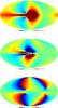 |
Fig. 8 Best-fit for the halo field by using the Stokes Q and U parameters and PA excluding the disk, the galactic center and the “loops” (ASS model with radial dependence). |
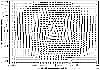 |
Fig. 9 Large-scale pattern of the best fit BSS+ model for the disk emission in the galactic disk (z = 0). |
4.3. Comparison of the result with the PA analysis
For comparison purposes, we also performed the analyses using the PA information alone. As discussed elsewhere, this analysis provides a limited amount of information because the PA is not sensitive to some parameters, like a constant field strength.
In general, the results using the PA provide compatible results to those of the Stokes Q and U analysis, although there is a larger number of unconstrained parameters and a poorer goodness-of-fit. To illustrate this, the ASS(r) analysis with mask 4 gives r1 < 45.9 kpc, p ~ 20.0°, and χ0 ~ 21.0° (χ2 ~ 2.3); while for the ASS case gives p ~ 20.5°, χ0 ~ 19.0° and no constraint on B0 (χ2 ~ 2.3). The pitch and tilt angles are compatible with those derived from the Stokes Q and U analysis. The best fit is given by the LSA with ψ0 > 22.3°, ψ1 > 8.6° and χ0 < 18.1° (χ2 ~ 2.3).
5. Conclusions
We have constrained the regular Galactic magnetic field by using the polarized emission at 22 GHz. To this aim we considered nine models of the Galactic magnetic field, each defined by three or four free parameters and for six different masks to interpret the polarized maps from WMAP5. The combination of models, free parameters, and masks produced a huge number of simulated maps to be compared with the observational ones in Stokes Q and U parameters, which in turn provide valuable constraints to determine the three dimensional configuration of the magnetic field of our Galaxy.
The family of GMF models that better describes the halo emission is the axisymmetric one, although any of the other considered models can be rejected based on their goodness-of-fit. The magnetic spiral arms have a pitch angle of p ≈ 24° and a tilt angle of χ0 ≈ 30°, implying a strong vertical field of ~1 μG at z = 1 kpc. When a radial variation is fitted, the models generally require a fast variation in the inner part of the galaxy (r1 < 2.5 kpc).
We stress that an accurate determination of the covariance matrix, which accounts for both the noise and the residual astrophysical components, is very complicated. We explored in detail three different methods and found that they may lead to differences of a factor of ~2−3 in the goodness-of-fit values, while the values of the best-fit parameters for each model do not vary significantly. In practice, this means that rejecting a model based on the goodness-of-fit could be inappropriate, although the relative differences of the χ2 statistic between models can be used for a comparison and for selecting preferred models.
We have also tried to constrain the disk field parameters using the polarized synchrotron emission, even though the fitted region is very small (~8% of the sky). Here, the obtained results are remarkably consistent with those obtained with other methods. In this case, all the considered models give a very similar goodness-of-fit, with a (very small) preference for an axisymmetric model. The data do not require a radial dependence of the strength, and the pitch angle values are much lower than in the halo case. Indeed, the constrained pitch angles are compatible with those found by using other observational methods like Faraday rotation of pulsars (Han et al. 2006) However, we note that this conclusion has not been reached by recent results where polarized synchrotron emission is used (see e.g. Jansson et al. 2009). The tilt angle in the disk is χ0 ~ 17°, which implies a vertical field structure with Bz ~ 0.1 μG at z = 200 pc. This value is compatible with that found by Han & Qiao (1994), based on the rotation measure of pulsars.
We remark that there are still some important uncertainties in the modeling of the synchrotron emission. In particular, we probably need a better knowledge of the distribution of cosmic rays, which is today a clear source of indeterminations in this type of analyses. The detailed modeling of the halo field could have an influence on the cosmic ray trajectories and could be crucial for the direct detection of the primordial magnetic fields.
Finally, we expect that the higher sensitivity and angular resolution in the polarized channels of the PLANCK telescope (The Planck Collaboration 2006; Tauber et al. 2010), the low-frequency channels of the QUIJOTE-CMB experiment (Rubiño-Martín et al. 2010) and experiments like LOFAR and SKA (Beck 2009b), will provide a greater improvement of our knowledge of the Galactic magnetic field.
The “pitch angle” is defined here as the angle between the azimuthal direction and the
magnetic field. The azimuthal direction ( )
increases anti-clockwise, so p is positive since the anti-clockwise
tangent to the spiral is outside the circle with radius r. Note that in
some works in the literature, the convention for the -angle is exactly opposite (i.e. it increases
clockwise). Finally, note that for the case p = 0°, the
solenoidal model is recovered.
)
increases anti-clockwise, so p is positive since the anti-clockwise
tangent to the spiral is outside the circle with radius r. Note that in
some works in the literature, the convention for the -angle is exactly opposite (i.e. it increases
clockwise). Finally, note that for the case p = 0°, the
solenoidal model is recovered.
The marginal distribution functions are obtained by integrating the joint distribution function over the variables that are discarded. For example, for the LSA model, the marginal distribution function for ℒ(ψ0) is derived by integrating the joint distribution ℒ(ψ0,ψ1,χ0) over ψ1 and χ0.
Note that these values are translated into our sign convention for the pitch angle.
Acknowledgments
We acknowledge Dr. Marco Tucci and Dr. Juan Betancort-Rijo for useful discussions and Dr. Ángel de Vicente for computing support. We acknowledge the MPIfR “magnetic group” and specially Prof. Richard Wielebinski for help and useful discussions. We acknowledge the use of the Legacy Archive for Microwave Background Data Analysis (LAMBDA). Support for LAMBDA is provided by the NASA Office of Space Science. Some of the results in this paper have been derived using the HEALPix Górski et al. (2005) package. To reduce the computational time needed for the production of the polarized synchrotron maps in this paper, we made use of the Condor workload management system (http://www.cs.wisc.edu/condor/) installed at the IAC. This project has been partially supported by Spanish MEC Grant ESP 2004-06870-C02. This work has been partially funded by project AYA2007-68058-C03-01 of the Spanish Ministry of Science and Innovation (MICINN). JAR-M is a Ramón y Cajal fellow of the MICINN.
References
- Abdo, A. A., Allen, B. T., Aune, T., et al. 2009, ApJ, 698, 2121 [Google Scholar]
- Battaner, E., & Florido, E. 1995, MNRAS, 277, 1129 [NASA ADS] [CrossRef] [Google Scholar]
- Battaner, E. & Florido, E. 2000, Fundamentals of Cosmic Physics, 21, 1 [Google Scholar]
- Battaner, E., & Florido, E. 2007, Astron. Nachr., 328, 92 [Google Scholar]
- Battaner, E. & Florido, E. 2009, in IAU Symp., 529 [Google Scholar]
- Battaner, E., Garrido, J. L., Membrado, M., & Florido, E. 1992, Nature, 360, 652 [NASA ADS] [CrossRef] [Google Scholar]
- Battaner, E., Castellano, J., & Masip, M. 2009, ApJ, 703, L90 [NASA ADS] [CrossRef] [Google Scholar]
- Beck, R. 2007, ed. M.-A. Miville-Deschênes, & F. Boulanger, EAS Publ. Ser., 23, 19 [Google Scholar]
- Beck, R. 2009a, IAU Symp., 259, 3 [Google Scholar]
- Beck, R. 2009b, Rev. Mex. Astron. Astrofis. Conf. Ser., 36, 1 [NASA ADS] [Google Scholar]
- Beck, R., Brandenburg, A., Moss, D., Shukurov, A., & Sokoloff, D. 1996, ARA&A, 34, 155 [NASA ADS] [CrossRef] [Google Scholar]
- Berkhuijsen, E. M., Haslam, C. G. T., & Salter, C. J. 1971, A&A, 14, 252 [NASA ADS] [Google Scholar]
- Beuermann, K., Kanbach, G., & Berkhuijsen, E. M. 1985, A&A, 153, 17 [NASA ADS] [Google Scholar]
- Bluemer, J., & for the Pierre Auger Collaboration 2008, Astropart. Phys., 29, 188 [Google Scholar]
- Bridle, S. L., Crittenden, R., Melchiorri, A., et al. 2002, MNRAS, 335, 1193 [NASA ADS] [CrossRef] [Google Scholar]
- Brown, J. C., Haverkorn, M., Gaensler, B. M., et al. 2007, ApJ, 663, 258 [NASA ADS] [CrossRef] [Google Scholar]
- Carretti, E., McConnell, D., Haverkorn, M., et al. 2008, Mapping the Galaxy and Nearby Galaxies, 93 [Google Scholar]
- Chandrasekhar, S. 1960, Radiative transfer, ed. S. Chandrasekhar [Google Scholar]
- Drimmel, R., & Spergel, D. N. 2001, ApJ, 556, 181 [NASA ADS] [CrossRef] [Google Scholar]
- Fish, V. L., Reid, M. J., Argon, A. L., & Menten, K. M. 2003, ApJ, 596, 328 [NASA ADS] [CrossRef] [Google Scholar]
- Gaensler, B. M., Dickey, J. M., McClure-Griffiths, N. M., et al. 2001, ApJ, 549, 959 [NASA ADS] [CrossRef] [Google Scholar]
- Górski, K. M., Hivon, E., Banday, A. J., et al. 2005, ApJ, 622, 759 [NASA ADS] [CrossRef] [Google Scholar]
- Han, J. 2009, IAU Symp., 259, 455 [NASA ADS] [Google Scholar]
- Han, J. L. 2001, Ap&SS, 278, 181 [NASA ADS] [CrossRef] [Google Scholar]
- Han, J. L. 2008a, in Astrophysics of Compact Objects, ed. Y.-F. Yuan, X.-D. Li, & D. Lai, AIP Conf. Ser., 968, 165 [Google Scholar]
- Han, J. L. 2008b, Nucl. Phys. B Proc. Suppl., 175, 62 [NASA ADS] [CrossRef] [Google Scholar]
- Han, J. L., & Qiao, G. J. 1994, A&A, 288, 759 [NASA ADS] [Google Scholar]
- Han, J. L. & Wielebinski, R. 2002, Chinese J. Astron. Astrophys., 2, 293 [Google Scholar]
- Han, J. L., & Zhang, J. S. 2007, A&A, 464, 609 [NASA ADS] [CrossRef] [EDP Sciences] [Google Scholar]
- Han, J. L., Manchester, R. N., Berkhuijsen, E. M., & Beck, R. 1997, A&A, 322, 98 [NASA ADS] [Google Scholar]
- Han, J. L., Manchester, R. N., & Qiao, G. J. 1999, MNRAS, 306, 371 [NASA ADS] [CrossRef] [Google Scholar]
- Han, J. L., Ferriere, K., & Manchester, R. N. 2004, ApJ, 610, 820 [NASA ADS] [CrossRef] [Google Scholar]
- Han, J. L., Manchester, R. N., Lyne, A. G., Qiao, G. J., & van Straten, W. 2006, ApJ, 642, 868 [NASA ADS] [CrossRef] [Google Scholar]
- Harari, D., Mollerach, S., & Roulet, E. 1999, J. High Energy Phys., 8, 22 [Google Scholar]
- Haverkorn, M., Brown, J. C., Gaensler, B. M., & McClure-Griffiths, N. M. 2008a, ApJ, 680, 362 [NASA ADS] [CrossRef] [Google Scholar]
- Haverkorn, M., Gaensler, B. M., & Brown, J.-A. C. 2008b, in Mapping the Galaxy and Nearby Galaxies, ed. K. Wada, & F. Combes, 329 [Google Scholar]
- Heiles, C. 1996, ApJ, 462, 316 [NASA ADS] [CrossRef] [Google Scholar]
- Hinshaw, G., Weiland, J. L., Hill, R. S., et al. 2009, ApJS, 180, 225 [NASA ADS] [CrossRef] [Google Scholar]
- Hou, L. G., Han, J. L., & Shi, W. B. 2009, A&A, 499, 473 [NASA ADS] [CrossRef] [EDP Sciences] [Google Scholar]
- Indrani, C. & Deshpande, A. A. 1999, New Astron., 4, 33 [NASA ADS] [CrossRef] [Google Scholar]
- Jansson, R., Farrar, G. R., Waelkens, A. H., et al. 2008, Int. Cosmic Ray Conf., 2, 223 [Google Scholar]
- Jansson, R., Farrar, G. R., Waelkens, A. H., & Enßlin, T. A. 2009, J. Cosmol. Astro-Part. Phys., 7, 21 [Google Scholar]
- Kutschera, M., & Jalocha, J. 2004, Acta Phys. Polonica B, 35, 2493 [NASA ADS] [Google Scholar]
- La Rosa, T. N., Shore, S. N., Joseph, T., Lazio, W., & Kassim, N. E. 2006, J. Phys. Conf. Ser., 54, 10 [NASA ADS] [CrossRef] [Google Scholar]
- Masip, M. & Mastromatteo, I. 2008, J. Cosmol. Astro-Part. Phys., 12, 3 [NASA ADS] [CrossRef] [Google Scholar]
- Men, H., Ferrière, K., & Han, J. L. 2008, A&A, 486, 819 [NASA ADS] [CrossRef] [EDP Sciences] [Google Scholar]
- Miville-Deschênes, M.-A., Ysard, N., Lavabre, A., Ponthieu, N., Macías-Pérez, J. F., Aumont, J., & Bernard, J. P. 2008, A&A, 490, 1093 [NASA ADS] [CrossRef] [EDP Sciences] [Google Scholar]
- Nelson, A. H. 1988, MNRAS, 233, 115 [NASA ADS] [Google Scholar]
- Noutsos, A., Johnston, S., Kramer, M., & Karastergiou, A. 2008, MNRAS, 386, 1881 [NASA ADS] [CrossRef] [Google Scholar]
- Page, L., Hinshaw, G., Komatsu, E., et al. 2007, ApJS, 170, 335 [NASA ADS] [CrossRef] [Google Scholar]
- Plante, R. L., Lo, K. Y., & Crutcher, R. M. 1995, ApJ, 445, L113 [NASA ADS] [CrossRef] [Google Scholar]
- Poezd, A., Shukurov, A., & Sokoloff, D. 1993, MNRAS, 264, 285 [NASA ADS] [CrossRef] [Google Scholar]
- Prouza, M., & Šmída, R. 2003, A&A, 410, 1 [NASA ADS] [CrossRef] [EDP Sciences] [Google Scholar]
- Rand, R. J., & Kulkarni, S. R. 1989, ApJ, 343, 760 [NASA ADS] [CrossRef] [Google Scholar]
- Reich, W. 2006, [arXiv:astro-ph/0603465] [Google Scholar]
- Roy, S., Pramesh Rao, A., & Subrahmanyan, R. 2008, A&A, 478, 435 [NASA ADS] [CrossRef] [EDP Sciences] [Google Scholar]
- Rubiño-Martín, J. A., et al. 2010, Highlights of Spanish Astrophysics V, 127 [Google Scholar]
- Rybicki, G. B., & Lightman, A. P. 1986, Radiat. Proc. Astrophys., ed. G. B. Rybicki, & A. P. Lightman [Google Scholar]
- Simard-Normandin, M., & Kronberg, P. P. 1980, ApJ, 242, 74 [NASA ADS] [CrossRef] [Google Scholar]
- Stanev, T. 1997, ApJ, 479, 290 [NASA ADS] [CrossRef] [Google Scholar]
- Strong, A. W., Moskalenko, I. V., & Ptuskin, V. S. 2007, Ann. Rev. Nucl. Part. Science, 57, 285 [Google Scholar]
- Sun, X. H., Reich, W., Waelkens, A., & Enßlin, T. A. 2008, A&A, 477, 573 [NASA ADS] [CrossRef] [EDP Sciences] [Google Scholar]
- Tauber, J., et al. 2010, A&A, 520, A1 [NASA ADS] [CrossRef] [EDP Sciences] [Google Scholar]
- Testori, J. C., Reich, P., & Reich, W. 2008, A&A, 484, 733 [NASA ADS] [CrossRef] [EDP Sciences] [Google Scholar]
- The Planck Collaboration 2006, [arXiv:astro-ph/0604069] [Google Scholar]
- Tinyakov, P. G., & Tkachev, I. I. 2002, Astropart. Phys., 18, 165 [NASA ADS] [CrossRef] [Google Scholar]
- Vallee, J. P. 1991, ApJ, 366, 450 [NASA ADS] [CrossRef] [Google Scholar]
- Vallee, J. P. 1995, ApJ, 454, 119 [CrossRef] [Google Scholar]
- Vallée, J. P. 2002, ApJ, 566, 261 [NASA ADS] [CrossRef] [Google Scholar]
- Vallée, J. P. 2008, ApJ, 681, 303 [NASA ADS] [CrossRef] [Google Scholar]
- Weisberg, J. M., Cordes, J. M., Kuan, B., et al. 2004, ApJS, 150, 317 [NASA ADS] [CrossRef] [Google Scholar]
- Wolleben, M., Landecker, T. L., Reich, W., & Wielebinski, R. 2006, A&A, 448, 411 [NASA ADS] [CrossRef] [EDP Sciences] [Google Scholar]
All Tables
Best-fit parameters for the global and halo component of the GMF model (masks 1, 2, 3, and 4), based on the analysis of the Stokes Q and U parameters.
All Figures
|
Fig. 1 Observed Stokes Q (top) and U (bottom) maps at 22 GHz from WMAP5 data. The maps are shown in a Mollweide projection of HEALPix in Galactic coordinates. The center of the map corresponds to (l,b) = (0°,0°), and the graticule increases with Δl = Δb = 45°. The maps are degraded to nside = 16 to enhance the large scale pattern. Units are mK (thermodynamic). |
| In the text | |
|
Fig. 2 Observed direction of the polarization angle (PA) at 22 GHz, obtained from the two maps shown in Fig. 1. The PA is defined here as the local direction of the magnetic field (see Eq. (10)). Units are degrees. |
| In the text | |
|
Fig. 3 Noise maps for the WMAP5 datasets presented in Figs. 1 and 2. They show the Stokes Q (top), Stokes U (middle) and position angle (PA, bottom) maps. Units for Stokes Q and U maps are mK. Units for the PA map are degrees. The noise map for PA has been computed as fluctuations around the observed WMAP5 K-band map. |
| In the text | |
|
Fig. 4 Regions used for the definition of the six masks adopted for the analyses (see text for details). |
| In the text | |
|
Fig. 5 Mask for the galactic polarized emission used by the WMAP team. |
| In the text | |
|
Fig. 6 Large-scale pattern of the ASS(r) model at z = 4 kpc. This model provides the best fit for the halo field. |
| In the text | |
|
Fig. 7 One dimensional (marginalized) posterior distribution functions for the parameters of ASS(r) halo model (top: r1, middle: p and bottom: χ0) when mask 4 is considered in the Stokes Q and U analysis. |
| In the text | |
|
Fig. 8 Best-fit for the halo field by using the Stokes Q and U parameters and PA excluding the disk, the galactic center and the “loops” (ASS model with radial dependence). |
| In the text | |
|
Fig. 9 Large-scale pattern of the best fit BSS+ model for the disk emission in the galactic disk (z = 0). |
| In the text | |
Current usage metrics show cumulative count of Article Views (full-text article views including HTML views, PDF and ePub downloads, according to the available data) and Abstracts Views on Vision4Press platform.
Data correspond to usage on the plateform after 2015. The current usage metrics is available 48-96 hours after online publication and is updated daily on week days.
Initial download of the metrics may take a while.