| Issue |
A&A
Volume 521, October 2010
|
|
|---|---|---|
| Article Number | A74 | |
| Number of page(s) | 18 | |
| Section | Galactic structure, stellar clusters, and populations | |
| DOI | https://doi.org/10.1051/0004-6361/201015222 | |
| Published online | 22 October 2010 | |
The wide variety of evolutionary stages
among 34 unstudied Teutsch open clusters![[*]](/icons/foot_motif.png)
C. Bonatto - E. Bica
Universidade Federal do Rio Grande do Sul,
Departamento de Astronomia CP 15051, RS, Porto Alegre
91501-970, Brazil
Received 16 June 2010 / Accepted 15 July
2010
Abstract
Context. Close investigations of unstudied
open-cluster candidates may improve the statistics of objects
undergoing the dissolution phase.
Aims. We plan to settle the nature and derive
astrophysical (fundamental, structural, and stellar mass content)
parameters for 34 unstudied open cluster candidates from the
near-infrared Teutsch list.
Methods. The analysis employs 2MASS photometry,
field-star decontamination (to enhance the intrinsic colour-magnitude
diagram morphology), and colour-magnitude filters (for high contrast in
stellar radial density profiles).
Results. We find 8 clusters younger than ![]() 30 Myr,
21 with ages within 100-900 Myr, 3 older than
1 Gyr, and possibly 1 as old as
30 Myr,
21 with ages within 100-900 Myr, 3 older than
1 Gyr, and possibly 1 as old as ![]() 7 Gyr.
Part of the sample is affected by reddening as high as
7 Gyr.
Part of the sample is affected by reddening as high as ![]() ,
and about half is located more than
,
and about half is located more than ![]() kpc
away from the Sun, with a few reaching
kpc
away from the Sun, with a few reaching ![]() kpc.
The sample contains essentially low-luminosity clusters in the optical,
with
kpc.
The sample contains essentially low-luminosity clusters in the optical,
with ![]() .
These properties are consistent with their near-infrared origin.
Cluster size increases both with Galactocentric distance and height
over the plane, which is consistent with the low level of tidal stress
(and field contamination) associated with these regions. The average
mass density falls off with cluster radius as
.
These properties are consistent with their near-infrared origin.
Cluster size increases both with Galactocentric distance and height
over the plane, which is consistent with the low level of tidal stress
(and field contamination) associated with these regions. The average
mass density falls off with cluster radius as ![]() ,
which in clusters younger than
,
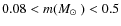
which in clusters younger than ![]() 20 Myr and more massive than
20 Myr and more massive than ![]()
![]() has been interpreted as diffusion-related cluster expansion.
has been interpreted as diffusion-related cluster expansion.
Conclusions. Besides the derivation of astrophysical
parameters for a sample of unstudied open clusters, in this paper we
identify a set of clusters older than several 102 Myr,
with 4 of them having survived a few Gyr. Surveys of
open cluster candidates should be further explored to fill in the gap
between the detected and predicted number of clusters. An improved
statistic, especially on the population of clusters in highly evolved
phases, can be used to investigate cluster formation rates and
constrain the dissolution-time scale in the Galaxy.
Key words: open clusters and associations: general - Galaxy: structure
1 Introduction
Star formation is a mass and size scale-free process that yields a
power-law mass distribution ![]() (e.g. Elmegreen 2008). Thus,
open cluster (OC) formation is biased towards low masses, and large
numbers of low-mass
OCs are expected to form. Indeed, estimates based on different
approaches (e.g.
Piskunov et al. 2006;
Bonatto et al. 2006)
consistently indicate that the Galaxy may harbour a population of
(e.g. Elmegreen 2008). Thus,
open cluster (OC) formation is biased towards low masses, and large
numbers of low-mass
OCs are expected to form. Indeed, estimates based on different
approaches (e.g.
Piskunov et al. 2006;
Bonatto et al. 2006)
consistently indicate that the Galaxy may harbour a population of ![]() 105 OCs.
However, widely-used databases, such as WEBDA
105 OCs.
However, widely-used databases, such as WEBDA![]() and the Catalog of Optically Visible Open Clusters and
Candidates
and the Catalog of Optically Visible Open Clusters and
Candidates![]() (Dias et al. 2002),
contain less than the 2000 OC candidates detected so far. Only
about half of these have unambiguously determined OC nature, and most
are located relatively close to the Sun and projected towards the
Galactic anti-centre. Given the high levels of field-star contamination
associated with large distances (particularly towards the bulge), part
of the detection problem is related to completeness, especially for the
low-mass OCs (Bonatto
et al. 2006). The OC fading associated with
the stellar evolution is also important.
(Dias et al. 2002),
contain less than the 2000 OC candidates detected so far. Only
about half of these have unambiguously determined OC nature, and most
are located relatively close to the Sun and projected towards the
Galactic anti-centre. Given the high levels of field-star contamination
associated with large distances (particularly towards the bulge), part
of the detection problem is related to completeness, especially for the
low-mass OCs (Bonatto
et al. 2006). The OC fading associated with
the stellar evolution is also important.
Most OCs dwell in or close to the Galactic disk and, because
of such orbits, they continually suffer tidal stress from Galactic
substructures, which produces different degrees of mass loss that might
lead to dissolution into the field. Over time, stellar
evolution-related mass loss, mass segregation and evaporation, tidal
interactions with the disk and/or bulge, and encounters with giant
molecular clouds, affect the critical balance between velocity
dispersion and escape velocity. These processes tend to accelerate the
dynamical evolution and change the internal cluster structure to
varying degrees, so that the vast majority of the OCs still
dissolve in the embedded phase (e.g. Lada
& Lada 2003). Theoretical and observational evidence
(e.g. Spitzer 1958; Oort 1958; Baumgardt
& Makino 2003; Goodwin
& Bastian 2006; Lamers
& Gieles 2006; Khalisi
et al. 2007; Piskunov
et al. 2007) point to a disruption time scale of a
few 102 Myr near the solar circle. As a
consequence, most OCs dissolve in the Galactic stellar field (e.g. Lamers et al. 2005) or
leave poorly-populated remnants (e.g. Pavani
& Bica 2007), long before ![]() 1 Gyr (e.g. Goodwin
& Bastian 2006).
1 Gyr (e.g. Goodwin
& Bastian 2006).
Probably because of the age/dissolution effect, only ![]()
![]() of the WEBDA OCs with known age are older than 1 Gyr, while
of the WEBDA OCs with known age are older than 1 Gyr, while ![]()
![]() are younger than 100 Myr. Besides the obvious importance of
deriving astrophysical parameters of unstudied clusters of any age, the
identification of OCs older than several 102 Myr
will thus increase the statistics of objects undergoing the dissolution
phase. This, in turn, can be used for constraining the dissolution-time
scale in the Galaxy.
are younger than 100 Myr. Besides the obvious importance of
deriving astrophysical parameters of unstudied clusters of any age, the
identification of OCs older than several 102 Myr
will thus increase the statistics of objects undergoing the dissolution
phase. This, in turn, can be used for constraining the dissolution-time
scale in the Galaxy.
In the present paper we investigate the nature of 34 unstudied
Teutsch (hereafter Teu) OC candidates and derive their astrophysical
parameters. In short, the analysis involves the following steps for
each cluster: (i) extraction of 2MASS photometry![]() (Skrutskie et al. 1997)
in a wide circular region; (ii) field-star decontamination to enhance
the intrinsic colour-magnitude diagram (CMD) morphology (essential for
a proper derivation of reddening, age, and distance from the Sun); and
(iii) construction of colour-magnitude filters, for more contrasted
stellar radial density profiles (RDPs). In previous works (e.g. Bica et al. 2008), we
have shown that steps (ii) and (iii) are essential
for a robust determination of fundamental parameters, especially for
low-latitude and/or bulge-projected OCs.
(Skrutskie et al. 1997)
in a wide circular region; (ii) field-star decontamination to enhance
the intrinsic colour-magnitude diagram (CMD) morphology (essential for
a proper derivation of reddening, age, and distance from the Sun); and
(iii) construction of colour-magnitude filters, for more contrasted
stellar radial density profiles (RDPs). In previous works (e.g. Bica et al. 2008), we
have shown that steps (ii) and (iii) are essential
for a robust determination of fundamental parameters, especially for
low-latitude and/or bulge-projected OCs.
Table 1: Fundamental parameters.
This paper is organised as follows. In Sect. 2 we discuss formation of the unstudied Teutsch sample. In Sect. 3 we present the 2MASS photometry and the field-star decontaminated CMDs. In Sect. 4 we discuss the derivation of fundamental cluster parameters. In Sect. 5 we investigate cluster structure. In Sect. 6 we present stellar mass estimates. In Sect. 7 we investigate relations among parameters and with respect to their location in the Galaxy. Concluding remarks are given in Sect. 8.
2 The sample of unstudied Teutsch clusters
After inspecting the Digitized Sky Survey (DSS) and 2MASS images of
selected Milky Way regions, Kronberger
et al. (2006) reported the discovery of several
stellar groupings with morphology, CMD, and stellar RDP, which suggest
uncatalogued, possible OCs. SIMBAD![]() lists 146 objects under the
designation of Teutsch OC candidates.
lists 146 objects under the
designation of Teutsch OC candidates.
Our first step was to search in the ``Catalog of Optically
Visible Open Clusters and Candidates''![]() (Dias et al. 2002)
and WEBDA for Teutsch objects that are still considered as candidates,
i.e.,
with no determination of their fundamental parameters. This survey came
up with 34 targets, for which a further object search in
SAO/NASA ADS confirmed that, besides the discovery work (Kronberger et al. 2006),
have not been subject to further investigation.
(Dias et al. 2002)
and WEBDA for Teutsch objects that are still considered as candidates,
i.e.,
with no determination of their fundamental parameters. This survey came
up with 34 targets, for which a further object search in
SAO/NASA ADS confirmed that, besides the discovery work (Kronberger et al. 2006),
have not been subject to further investigation.
Images of the Teutsch clusters that came up from this search
are shown in Appendix A.
The images are centred on slightly different coordinates
(Table 1)
than those given in Dias
et al. (2002). By default, we always assume
the original coordinates to centre the 2MASS photometry extraction.
However, in most cases the RDPs built after field decontamination - to
maximise membership probability (Sect. 3), presented a dip
in the innermost radial bin, so the central coordinates were computed
again according to the following strategy. After field
decontamination, we divided the central (usually ![]() in radius) region in cells of
in radius) region in cells of ![]() width both in right ascension and declination. Then, for each cell we
built an RDP using its coordinates as the centre. After repeating the
last step for all cells, we searched through the full RDP set for the
most cluster-like one, i.e., the one that maximises the stellar density
in the innermost bin, followed by a rather smooth decrease towards
large radii (Sect. 5).
Finally, we adopted these cell coordinates as the cluster's central
position. Incidentally, differences in the central coordinates are
relatively small for the present sample
(Table 1).
width both in right ascension and declination. Then, for each cell we
built an RDP using its coordinates as the centre. After repeating the
last step for all cells, we searched through the full RDP set for the
most cluster-like one, i.e., the one that maximises the stellar density
in the innermost bin, followed by a rather smooth decrease towards
large radii (Sect. 5).
Finally, we adopted these cell coordinates as the cluster's central
position. Incidentally, differences in the central coordinates are
relatively small for the present sample
(Table 1).
3 Photometric analysis
2MASS provides the spatial and photometric uniformity that are
essential for wide angular extractions. This in turn provides the high
star-count statistics required for the determination of the background
level (Sect. 5)
and the colour/magnitude characterisation of the field stars (see
below). In all cases we extracted the 2MASS photometry from VizieR![]() , in a circular field of
radius
, in a circular field of
radius ![]() .
To preserve the photometric quality and, at the same time, keep
a statistically significant number of stars, we use only photometric
errors in J, H, and
.
To preserve the photometric quality and, at the same time, keep
a statistically significant number of stars, we use only photometric
errors in J, H, and ![]() that are lower than 0.15 mag. Reddening corrections are based
on the absorption relations AJ/AV=0.276,
AH/AV=0.176,
that are lower than 0.15 mag. Reddening corrections are based
on the absorption relations AJ/AV=0.276,
AH/AV=0.176,
![]() ,
and
,
and ![]() given by Dutra et al. (2002),
with RV=3.1,
considering the extinction curve of Cardelli
et al. (1989).
given by Dutra et al. (2002),
with RV=3.1,
considering the extinction curve of Cardelli
et al. (1989).
The clusters are distributed over all Galactic quadrants (Table 1), so that field-stars are expected to contaminate the CMDs at different degrees, usually high in the 1st and 2nd quadrants and low in the 3rd and 4th (e.g. Bonatto et al. 2006). Also, since most of the clusters are relatively poorly populated (Figs. 1-7), the field-star contamination should be taken into account so that the derived parameters are more constrained. In particular, we expect to obtain CMDs in which clusters' evolutionary sequences and field stars are reasonably disentangled.
|
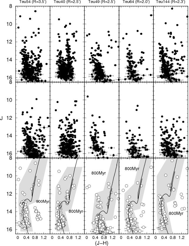
Figure 1: CMDs of Teu 54, 40, 49, 64, and 144 for a representative cluster region (top panels) and the equal-area comparison field (middle). The decontaminated CMDs (bottom) are shown with the isochrone solution (solid line) and the colour-magnitude filter (shaded polygon). |
| Open with DEXTER | |
|
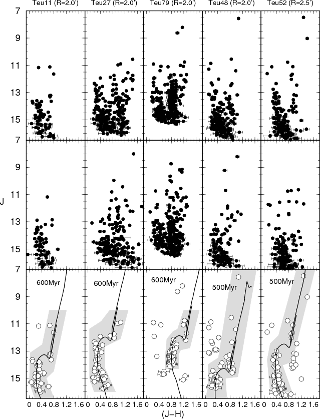
Figure 2: Same as Fig. 1 for Teu 11, 27, 79, 48, and 52. |
| Open with DEXTER | |
|
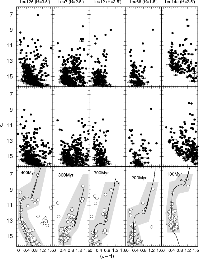
Figure 3: Same as Fig. 1 for Teu 126, 7, 12, 66, and 14a. |
| Open with DEXTER | |
|
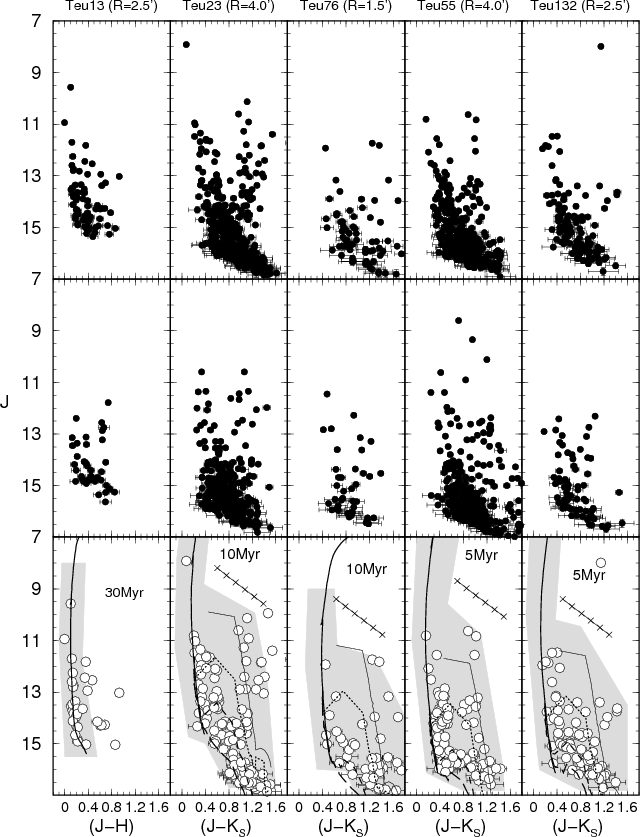
Figure 4:
Same as Fig. 1
for Teu 13 ( left panel). The remaining
clusters
(Teu 23, 7, 76, 55, and 132) are shown in |
| Open with DEXTER | |
|
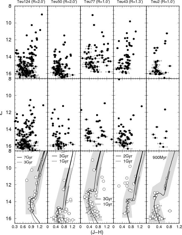
Figure 5: Same as Fig. 1 for Teu 124, 50, 77, 43, and 2. Isochrones younger than the adopted ones are also shown for an estimate of a lower limit to the age. |
| Open with DEXTER | |
|
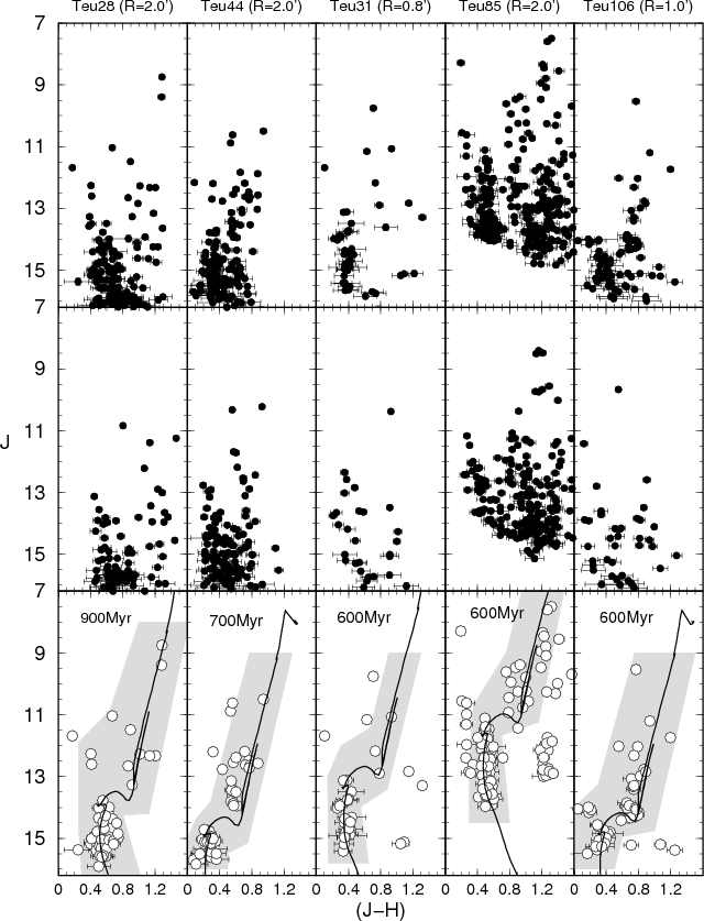
Figure 6: Same as Fig. 1 for Teu 28, 44, 31, 85, and 106. |
| Open with DEXTER | |
|
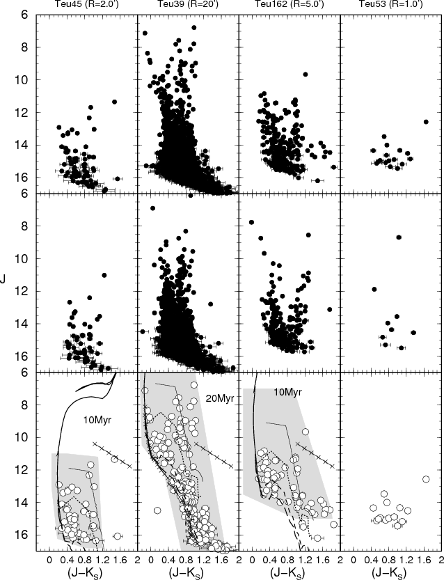
Figure 7:
Same as Fig. 1
but with |
| Open with DEXTER | |
For this purpose we work with the statistical decontamination algorithm
that has been developed by our group for the proper identification and
characterisation of star clusters, especially near the Galactic equator
and/or with many faint stars. We start by defining the cluster and
comparison field regions![]() ,
taken within the wide circular extractions. CMDs extracted within the
cluster region for our objects are shown in Figs. 1-7
(top panels), which should be contrasted with the representative (i.e.
equal-area)
comparison-field CMDs (middle panels). The equal-area field extractions
are only used for qualitative comparisons, since the algorithm uses the
whole surrounding area (as defined above) for high statistical
representativeness. For most stars the error bars are smaller than the
symbol. Our approach assumes that the field colour-magnitude
distribution is (i) statistically representative of the cluster
contamination; and (ii) presents some degree of spatial uniformity.
These assumptions are usually matched in the 3rd and 4th Galactic
quadrants. More details on the decontamination algorithm are in Bonatto & Bica (2007b) and Bonatto & Bica (2010a). For
clarity,
we sketch how it works.
,
taken within the wide circular extractions. CMDs extracted within the
cluster region for our objects are shown in Figs. 1-7
(top panels), which should be contrasted with the representative (i.e.
equal-area)
comparison-field CMDs (middle panels). The equal-area field extractions
are only used for qualitative comparisons, since the algorithm uses the
whole surrounding area (as defined above) for high statistical
representativeness. For most stars the error bars are smaller than the
symbol. Our approach assumes that the field colour-magnitude
distribution is (i) statistically representative of the cluster
contamination; and (ii) presents some degree of spatial uniformity.
These assumptions are usually matched in the 3rd and 4th Galactic
quadrants. More details on the decontamination algorithm are in Bonatto & Bica (2007b) and Bonatto & Bica (2010a). For
clarity,
we sketch how it works.
A cluster CMD is divided into a 3D grid of cells with axes
along the J magnitude and the (J-H)
and ![]() colours, with initial dimensions
colours, with initial dimensions ![]() and
and ![]() .
Then, we compute the probability that a given star is found in a
particular cell. For a star with measured magnitude and colour
uncertainties
.
Then, we compute the probability that a given star is found in a
particular cell. For a star with measured magnitude and colour
uncertainties ![]() ,
,
![]() ,
and
,
and ![]() ,
the probability is proportional to the difference between the error
function computed at the borders of the cell. This step is taken for
all stars and cells, resulting in a number density of
,
the probability is proportional to the difference between the error
function computed at the borders of the cell. This step is taken for
all stars and cells, resulting in a number density of ![]() stars for each cell (
stars for each cell (
![]() ).
The same steps are applied to the comparison field CMD, from which we
estimate the field number density (
).
The same steps are applied to the comparison field CMD, from which we
estimate the field number density (
![]() )
for each cell. Next, we subtract the corresponding field number density
for each cluster cell to obtain a decontaminated number density (
)
for each cell. Next, we subtract the corresponding field number density
for each cluster cell to obtain a decontaminated number density (
![]() ).
Finally,
).
Finally, ![]() is converted back into number of stars and subtracted from each cell,
and the
is converted back into number of stars and subtracted from each cell,
and the ![]() stars that remain in the cell are identified. We also compute the
subtraction efficiency (
stars that remain in the cell are identified. We also compute the
subtraction efficiency (
![]() ), which is the sum over all
cells of the difference between the expected number of field stars
(usually fractional) and the number of stars effectively subtracted
(integer). In all cases we obtained
), which is the sum over all
cells of the difference between the expected number of field stars
(usually fractional) and the number of stars effectively subtracted
(integer). In all cases we obtained ![]() .
.
The above procedure is repeated for 729 different setups
(taking independent variations of cell size and grid positioning into
account). Each setup produces a total number of member stars ![]() ,
from which we compute the expected total number of member stars
,
from which we compute the expected total number of member stars ![]() by averaging out
by averaging out ![]() over all setups. Stars (identified above) are ranked according to the
number of times they survive all runs, and only the
over all setups. Stars (identified above) are ranked according to the
number of times they survive all runs, and only the ![]() highest ranked stars are considered cluster members and transposed to
the respective decontaminated CMD.
The decontaminated CMDs of the present sample are shown in
Figs. 1-7 (bottom panels).
highest ranked stars are considered cluster members and transposed to
the respective decontaminated CMD.
The decontaminated CMDs of the present sample are shown in
Figs. 1-7 (bottom panels).
Finally, we classify each case as Quality 1, 2, or 3 according to a subjective analysis based on how cluster-like the image (Appendix A), decontaminated CMD (Figs. 1-7), and RDP (Sect. 5) are.
4 Derivation of fundamental parameters
The decontaminated CMD morphology, coupled to Padova isochrones (Girardi et al. 2002)
computed with the 2MASS filters![]() ,
are used
to derive the fundamental parameters (reddening, age, and distance from
the Sun). These isochrones are very similar to the Johnson-Kron-Cousins
ones (e.g. Bessel & Brett
1988), with differences of at most 0.01 mag in
colour (Bonatto et al. 2004).
With respect to metallicity, the difference between, e.g. solar and
subsolar metallicity isochrones for a given age is small, to within the
2MASS photometric uncertainties (Appendix 8). Thus, we adopt the
solar metallicity for simplicity.
,
are used
to derive the fundamental parameters (reddening, age, and distance from
the Sun). These isochrones are very similar to the Johnson-Kron-Cousins
ones (e.g. Bessel & Brett
1988), with differences of at most 0.01 mag in
colour (Bonatto et al. 2004).
With respect to metallicity, the difference between, e.g. solar and
subsolar metallicity isochrones for a given age is small, to within the
2MASS photometric uncertainties (Appendix 8). Thus, we adopt the
solar metallicity for simplicity.
A first look at the decontaminated CMDs suggests OCs in a wide variety of evolutionary stages (bottom panels of Figs. 1-7). In particular, the presence of somewhat distant and evolved (in different degrees) OCs is suggested by the giant clumps and red giant branches that show up in a significant fraction of the sample clusters (Figs. 1-3, 5, 6). On the other hand, young clusters are also seen that still contain PMS stars (Figs. 4 and 7).
With respect to the derivation of fundamental parameters,
several sophisticated approaches for analytical CMD fitting are
available (a summary is in Naylor
& Jeffries 2006).
However, for simplicity we adopt a more direct approach that compares
isochrones and the decontaminated CMD morphology. Specifically, the
solutions are searched by eye, using the combined
main sequence (MS) and evolved stellar distributions (or the PMS
for the young clusters) as constraint. Variations due to photometric
uncertainties (which are usually small, because of the restrictions
imposed in Sect. 3)
and the presence of binaries (which tend to produce a redwards bias in
the MS) are also taken into account. Starting with the isochrones set
for zero distance modulus and reddening, we shift them in magnitude and
colour until a satisfactory match![]() with the CMD is obtained. The best fits, according
to this approach, are shown in Figs. 1-7
(bottom panels), and the respective parameters are given in
Table 1.
with the CMD is obtained. The best fits, according
to this approach, are shown in Figs. 1-7
(bottom panels), and the respective parameters are given in
Table 1.
Open clusters younger than ![]() 30 Myr are expected to be affected by
differential reddening. Indeed, as shown by, e.g. Yadav
& Sagar (2001), the differential
reddening tends to increase towards younger ages, in some cases
reaching
30 Myr are expected to be affected by
differential reddening. Indeed, as shown by, e.g. Yadav
& Sagar (2001), the differential
reddening tends to increase towards younger ages, in some cases
reaching ![]() mag,
or
mag,
or ![]() mag.
Since we cannot derive the extinction for individual stars with 2MASS
photometry, we examine the effect of differential reddening simply by
means of a reddening vector (Figs. 4
and 7)
for
mag.
Since we cannot derive the extinction for individual stars with 2MASS
photometry, we examine the effect of differential reddening simply by
means of a reddening vector (Figs. 4
and 7)
for ![]() mag,
which surpasses the upper limit of Yadav
& Sagar (2001). Thus, most of the scatter, especially
in the PMS, can be accounted
for by differential reddening. Consequently, it is impossible to assign
a precise mass value for each PMS star (Sect. 6).
mag,
which surpasses the upper limit of Yadav
& Sagar (2001). Thus, most of the scatter, especially
in the PMS, can be accounted
for by differential reddening. Consequently, it is impossible to assign
a precise mass value for each PMS star (Sect. 6).
We find that 7 clusters are younger than ![]() 50 Myr,
6 of which still harbour a varying fraction of PMS stars. Among the
remaining, 21 have
ages within 100-900 Myr, while 4 appear to be older
than 1 Gyr (see
below). With respect to the distance from the Sun, they are distributed
as near as
50 Myr,
6 of which still harbour a varying fraction of PMS stars. Among the
remaining, 21 have
ages within 100-900 Myr, while 4 appear to be older
than 1 Gyr (see
below). With respect to the distance from the Sun, they are distributed
as near as ![]() kpc,
with a few more distant than
kpc,
with a few more distant than ![]() kpc,
and reaching distances as far as
kpc,
and reaching distances as far as ![]() kpc.
We'll return to this
point in Sect. 7.
kpc.
We'll return to this
point in Sect. 7.
From a comparison with CMDs of known OCs, Kronberger
et al. (2006) provide estimates for the distance
from the Sun and reddening for Teu 43 (
![]() kpc,
kpc,
![]() ),
Teu 48 (
),
Teu 48 (
![]() kpc,
kpc,
![]() ),
and Teu 79 (
),
and Teu 79 (
![]() kpc,
kpc,
![]() ).
While our values for Teu 48 are comparable, they are
very different for the other clusters. Given the decontaminated CMDs of
Teu 43 (Fig. 5),
Teu 48, and Teu 79 (Fig. 2), the age (and
consequently, the reddening and distance) is rather constrained to
within the quoted errors in Table 1. A probable source
for such differences is the lack of field star decontamination in the
analysis of Kronberger et al.
(2006).
).
While our values for Teu 48 are comparable, they are
very different for the other clusters. Given the decontaminated CMDs of
Teu 43 (Fig. 5),
Teu 48, and Teu 79 (Fig. 2), the age (and
consequently, the reddening and distance) is rather constrained to
within the quoted errors in Table 1. A probable source
for such differences is the lack of field star decontamination in the
analysis of Kronberger et al.
(2006).
Finally, it should be noted that in some cases in which the
observed CMDs present similarities, the age estimates contrast, as for
Teu 126 (![]() 400 Myr;
Fig. 3)
and Teu 55 (
400 Myr;
Fig. 3)
and Teu 55 (![]() 5 Myr;
Fig. 4).
Although the similarity between the observed CMDs (top panels), the
decontaminated ones (bottom)
are significantly different, with Teu 126 displaying a rather
well-populated and long MS, together with the typical ``redwards
bending'' of clusters a few 108 yr old.
In contrast, Teu 55 presents a nearly vertical and short MS
with a distribution of PMS-like stars. In addition, both objects show
different aspects in their optical
images (Sect. A),
with evidence of dust in Teu 55, which is consistent with our
age estimates for both objects.
5 Myr;
Fig. 4).
Although the similarity between the observed CMDs (top panels), the
decontaminated ones (bottom)
are significantly different, with Teu 126 displaying a rather
well-populated and long MS, together with the typical ``redwards
bending'' of clusters a few 108 yr old.
In contrast, Teu 55 presents a nearly vertical and short MS
with a distribution of PMS-like stars. In addition, both objects show
different aspects in their optical
images (Sect. A),
with evidence of dust in Teu 55, which is consistent with our
age estimates for both objects.
4.1 Interesting cases
The majority of the present Teutsch clusters are quite normal
in terms of
age; i.e., they are younger than 1 Gyr. However, we find 4
cases for which the CMDs indicate ages of a few Gyr. They are
Teu 43, 50, 77, and 124 (Fig. 5). Along with their
images (Appendix A),
the decontaminated CMDs are typical of old clusters, especially
Teu 124. Indeed, the isochrones that best represent the CMDs
of Teu 43, 50, and 77 indicate ages of 2 and
3 Gyr. Clearly, these clusters are older than 1 Gyr,
as shown by the rather inconsistent - when compared to the adopted fits
- and tentative solutions with younger isochrones. The CMD of
Teu 124 indicates a significantly older cluster, for which we
estimate the age 7-3+2 Gyr.
Again, the CMD morphology indicates that Teu 124 cannot be
younger than ![]() 3 Gyr.
3 Gyr.
The only object for which we could not find a satisfactory CMD
solution
is Teu 53 (Fig. 7).
As suggested by its image (Appendix A), it probably is a
very distant, poorly-populated cluster, with about 20 faint
stars distributed in a region of ![]()
![]() in radius. Both the observed and decontaminated CMDs
do not allow any inference on age. The RDP (Fig. 9) shows a density
excess for
in radius. Both the observed and decontaminated CMDs
do not allow any inference on age. The RDP (Fig. 9) shows a density
excess for ![]() ,
but it does not follow any analytical cluster profile (Sect. 5). Clearly,
Teu 53 requires deeper photometry for a proper analysis.
,
but it does not follow any analytical cluster profile (Sect. 5). Clearly,
Teu 53 requires deeper photometry for a proper analysis.
Finally, the decontaminated CMDs of Teu 52, 54, and
85 appear to display a second, reddened MS or giant clump. To a lesser
degree, the same applies to Teu 126. Since Teu 85 is
projected not far from the Galactic centre
(
![]() ,
,
![]() ),
this feature may be an artifact of the decontamination algorithm
associated with the high stellar background and
spatial variation of the extinction towards the bulge. The other OCs,
on the other hand, are located in the
),
this feature may be an artifact of the decontamination algorithm
associated with the high stellar background and
spatial variation of the extinction towards the bulge. The other OCs,
on the other hand, are located in the ![]() quadrant, which minimises the possibility
of a decontamination artifact. Alternatively, that feature might
suggest a more distant cluster (not seen in the respective images shown
in Appendix A)
caught in the line of sight. Deeper photometry would be required to
settle this point.
quadrant, which minimises the possibility
of a decontamination artifact. Alternatively, that feature might
suggest a more distant cluster (not seen in the respective images shown
in Appendix A)
caught in the line of sight. Deeper photometry would be required to
settle this point.
5 Cluster structure
Structural parameters are derived by means of the RDPs. We start by
using the decontaminated CMD morphologies and corresponding isochrone
solutions (Figs. 1-7) to build a
colour-magnitude filter for each cluster. Noise in the RDPs is
minimised when stars with colours (and magnitude) that are
clearly discordant of those assumed to represent the cluster![]() are excluded. Also, the
contrast with the background is enhanced (e.g.
Bonatto & Bica 2007b).
are excluded. Also, the
contrast with the background is enhanced (e.g.
Bonatto & Bica 2007b).
Table 2: Structural parameters derived from the RDPs.
|
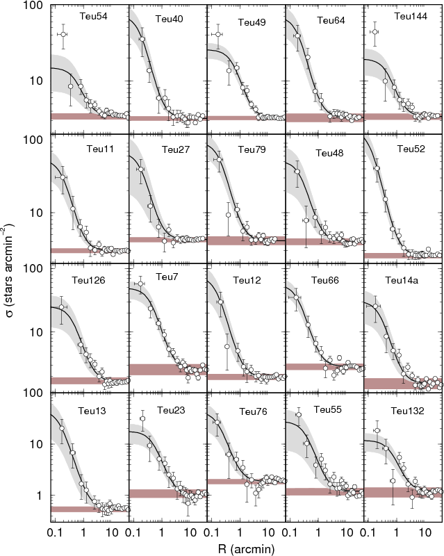
Figure 8:
Stellar RDPs (empty circles), the best-fit King-like profile (solid
line), the |
| Open with DEXTER | |
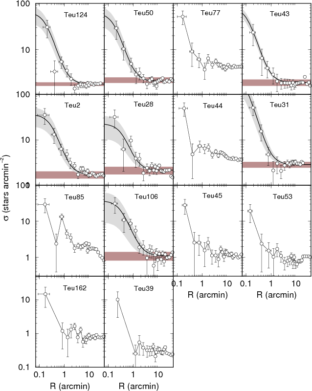
|
Figure 9: Same as Fig. 8 for the remaining clusters. It was not possible to fit the King-like profile for some cases. |
| Open with DEXTER | |
Table 3: Stellar mass estimate.
When the RDPs are built in rings of increasing width with
distance from the cluster centre, the spatial resolution is preserved
along the full radial range with moderate error bars. Specifically, we
use ![]() ,
respectively for
,
respectively for ![]() ,
,
![]() ,
,
![]() ,
,
![]() ,
and
,
and ![]() .
Obviously, for any magnitude
bin, field stars with the same colour as the cluster's are not excluded
by the filtering process. This residual background level is evaluated
as the average number density of stars in the comparison field. We take
the R coordinate (and uncertainty) of each
ring as the average position (and standard deviation) of the stars
inside the ring. The resulting RDPs (and residual background) are shown
in Figs. 8,
9. By measuring
the distance from the cluster centre where the RDP and residual
background are statistically indistinguishable, we get an estimate of
the cluster radius (
.
Obviously, for any magnitude
bin, field stars with the same colour as the cluster's are not excluded
by the filtering process. This residual background level is evaluated
as the average number density of stars in the comparison field. We take
the R coordinate (and uncertainty) of each
ring as the average position (and standard deviation) of the stars
inside the ring. The resulting RDPs (and residual background) are shown
in Figs. 8,
9. By measuring
the distance from the cluster centre where the RDP and residual
background are statistically indistinguishable, we get an estimate of
the cluster radius (
![]() ). Thus,
). Thus, ![]() can be considered as an observational truncation radius, whose value
depends both on the radial distribution of member stars and the field
density.
can be considered as an observational truncation radius, whose value
depends both on the radial distribution of member stars and the field
density.
The RDPs are fitted with the function ![]() ,
where
,
where ![]() and
and ![]() are the central and residual background stellar densities, and
are the central and residual background stellar densities, and ![]() is the core radius. Applied to star counts, this function is similar to
the one used by King (1962)
to describe surface-brightness profiles in the central parts of
globular clusters. Degrees of freedom are minimised by allowing only
is the core radius. Applied to star counts, this function is similar to
the one used by King (1962)
to describe surface-brightness profiles in the central parts of
globular clusters. Degrees of freedom are minimised by allowing only ![]() and
and ![]() to vary in the fits, while
to vary in the fits, while ![]() is previously measured in the surrounding field and kept fixed. The
best-fit solutions are shown in Figs. 8-9, and the structural
parameters are given in Table 2.
is previously measured in the surrounding field and kept fixed. The
best-fit solutions are shown in Figs. 8-9, and the structural
parameters are given in Table 2.
Within uncertainties, the adopted King-like function provides
a reasonable description
along the full radial range of the RDPs for most (![]()
![]() )
of the sample. The
exceptions are Teu 39, 44, 45, 53, 77, 85, and 162, which
present irregular RDPs that cannot be fitted by the adopted profile.
Also, Teu 54 (
)
of the sample. The
exceptions are Teu 39, 44, 45, 53, 77, 85, and 162, which
present irregular RDPs that cannot be fitted by the adopted profile.
Also, Teu 54 (
![]() Myr) and
Teu 144 (
Myr) and
Teu 144 (![]() 800 Myr)
present a pronounced density enhancement in the innermost RDP bin. This
feature has been attributed to a post-core collapse structure in some
globular clusters (e.g. Trager
et al. 1995). Such a dynamical evolution-related
feature
800 Myr)
present a pronounced density enhancement in the innermost RDP bin. This
feature has been attributed to a post-core collapse structure in some
globular clusters (e.g. Trager
et al. 1995). Such a dynamical evolution-related
feature![]() has also been detected in
the RDP of some Gyr-old OCs, e.g. NGC 3960 (Bonatto
& Bica 2006) and LK 10 (Bonatto
& Bica 2009a).
has also been detected in
the RDP of some Gyr-old OCs, e.g. NGC 3960 (Bonatto
& Bica 2006) and LK 10 (Bonatto
& Bica 2009a).
Compared to the distribution of core radii derived for a
sample of relatively nearby OCs by Piskunov et al. (2007,
their Fig. 3), the present clusters occupy the small-![]() tail. Finally, given the 2MASS photometric limit and the range of
distances spanned by the present cluster sample (Table 1), it is clear that
our analysis
does not include considerable (and varying) fractions of the low-mass
MS. The effect of
depth-limited photometry on the derivation of structural parameters has
been fully discussed by, e.g., Bonatto
& Bica (2008a). One conclusion is that, when the
2MASS photometry reaches a few magnitudes below the MS, the
depth-limited 2MASS photometry may underestimate
tail. Finally, given the 2MASS photometric limit and the range of
distances spanned by the present cluster sample (Table 1), it is clear that
our analysis
does not include considerable (and varying) fractions of the low-mass
MS. The effect of
depth-limited photometry on the derivation of structural parameters has
been fully discussed by, e.g., Bonatto
& Bica (2008a). One conclusion is that, when the
2MASS photometry reaches a few magnitudes below the MS, the
depth-limited 2MASS photometry may underestimate
![]() by less than
by less than ![]()
![]() .
The core radius (derived by means of the King-like fit), on the other
hand, may be underestimated by
.
The core radius (derived by means of the King-like fit), on the other
hand, may be underestimated by ![]()
![]() (OCs younger than
(OCs younger than ![]() 10 Myr)
and
10 Myr)
and ![]()
![]() (OCs older than
(OCs older than ![]() 1 Gyr).
Thus, our conclusions with respect
to the structural radii are not significantly affected by the 2MASS
depth limit.
1 Gyr).
Thus, our conclusions with respect
to the structural radii are not significantly affected by the 2MASS
depth limit.
6 Cluster mass estimate
As a consequence of combining the somewhat limited 2MASS photometric
depth with the relatively large distance of several of our OCs
(Table 1),
the CMDs in Figs. 1-7 do not contain the
whole mass range expected especially for OCs older than a few 107 Myr.
Thus, we estimate the stellar mass by means of the mass function (MF),
built for the observed MS mass range according to Bonatto
& Bica (2006). The MS MF is then fitted with the
function ![]() .
Results of this approach are given in Table 3, where we also show
the number and mass of the evolved stars. In most cases the detected MS
mass range is restricted to
.
Results of this approach are given in Table 3, where we also show
the number and mass of the evolved stars. In most cases the detected MS
mass range is restricted to ![]()
![]() ,
with a few cases reaching
,
with a few cases reaching ![]()
![]() .
Thus, assuming that the low-mass content is still present, we combine
our MF with Kroupa's (2001) MF
.
Thus, assuming that the low-mass content is still present, we combine
our MF with Kroupa's (2001) MF![]() to estimate the total stellar mass, down to the H-burning mass limit (
to estimate the total stellar mass, down to the H-burning mass limit (
![]() ).
When the MS is
determined well over a relatively large mass interval, we use our MF
over that mass
range and Kroupa's (2001) MF for lower masses. However, in some cases -
usually the oldest and/or distant OCs - the MS MF is excessively noisy.
In these cases we straightforwardly adopted Kroupa's (2001) MF, under
the condition that the MF, integrated over the detected MS mass range,
gives the observed number of stars. The (extrapolated)
cluster mass is given in Col. 8 of Table 3. Finally, having
estimated the cluster radius and mass, we also computed the average
cluster mass density
).
When the MS is
determined well over a relatively large mass interval, we use our MF
over that mass
range and Kroupa's (2001) MF for lower masses. However, in some cases -
usually the oldest and/or distant OCs - the MS MF is excessively noisy.
In these cases we straightforwardly adopted Kroupa's (2001) MF, under
the condition that the MF, integrated over the detected MS mass range,
gives the observed number of stars. The (extrapolated)
cluster mass is given in Col. 8 of Table 3. Finally, having
estimated the cluster radius and mass, we also computed the average
cluster mass density
![]() (Col. 9).
(Col. 9).
For the OCs with conspicuous PMS, we simply count the number
of MS stars and, for each star, we take the corresponding mass value
from the adopted isochrone. Differential reddening makes it impossible
to attribute a precise mass value to each PMS star. Thus, we again
count the number of PMS stars and adopt an average mass value
for the PMS stars to estimate ![]() and
and ![]() .
Assuming that the mass distribution of the PMS stars also follows
Kroupa's (2001) MF, the average PMS mass - for masses within the range
.
Assuming that the mass distribution of the PMS stars also follows
Kroupa's (2001) MF, the average PMS mass - for masses within the range ![]() - is
- is ![]() .
Thus, we simply multiply the number of PMS stars (Table 4) by this value to
estimate the PMS mass. Finally, we add the latter value to the MS mass
to obtain an estimate of the total stellar mass. Obviously,
similar to the MS stars, 2MASS cannot detect the very low-mass PMS
stars. Consequently, these values should be taken as lower limits.
.
Thus, we simply multiply the number of PMS stars (Table 4) by this value to
estimate the PMS mass. Finally, we add the latter value to the MS mass
to obtain an estimate of the total stellar mass. Obviously,
similar to the MS stars, 2MASS cannot detect the very low-mass PMS
stars. Consequently, these values should be taken as lower limits.
Table 4: Stellar mass estimate for the clusters with PMS.
7 Discussion
The fundamental and structural parameters derived in the previous sections can be used to compare the present Teutsch sample among the wide variety of OCs found in the literature. In particular, we wish to examine the representativeness of the present sample with respect to the Galactic OCs.
|
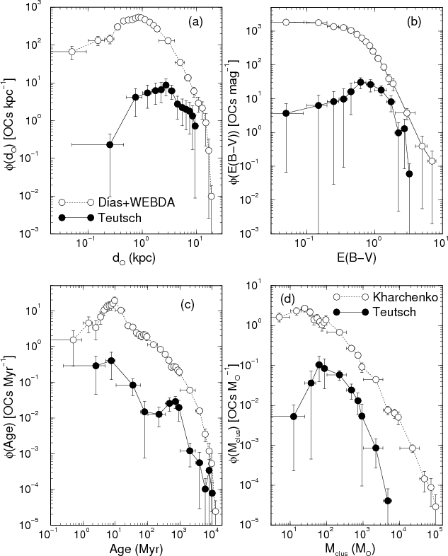
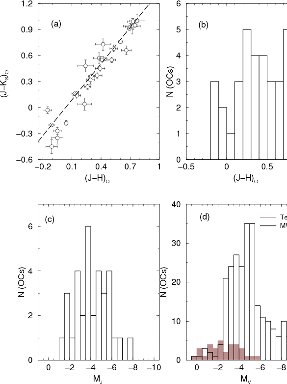
Figure 10: General properties of the present OCs (filled circles) compared to Galactic clusters (empty circles) taken from Dias et al. (2002) and WEBDA (panels a), b), and c)), and Piskunov et al. (2008) d). All cases are investigated with distribution functions. |
| Open with DEXTER | |
7.1 General properties
We start by considering the distance from the Sun, reddening, age, and
cluster mass distribution functions (Fig. 10). For the first
three parameters we take values from Dias
et al. (2002) and WEBDA, corresponding to about
1100 OCs. However, since neither database deals with cluster
mass, we use the uniform, semi-empirical mass determination for
650 OCs of Piskunov
et al. (2008). Qualitatively,
the Teutsch sample presents similar distributions to the Galactic OCs,
especially
with respect to the age. The same applies to cluster mass (especially
for masses higher than ![]()
![]() ),
although Piskunov et al.
(2008) includes OC masses as
high as
),
although Piskunov et al.
(2008) includes OC masses as
high as ![]()
![]() .
.
7.2 Location in the Galaxy
The present Teutsch clusters are shown projected onto the Galactic
plane in Fig. 11,
which depicts Milky Way's spiral arms according to Momany
et al. (2006) and Drimmel
& Spergel (2001). This structure was derived from HII
regions and molecular clouds (e.g. Russeil
2003); the Galactic bar is shown with an orientation
of 14![]() and 6 kpc of total length (Freudenreich
1998; Vallée 2005).
We also show, for comparison, the WEBDA OCs with known age and distance
from the Sun separated in two age groups of clusters younger or older
than 1 Gyr.
and 6 kpc of total length (Freudenreich
1998; Vallée 2005).
We also show, for comparison, the WEBDA OCs with known age and distance
from the Sun separated in two age groups of clusters younger or older
than 1 Gyr.
Figure 11
shows that all directions present a decreasing number of detected OCs
for distances farther than ![]() 2 kpc
from the Sun. This can be explained by completeness (due to crowding
and high background levels) and enhanced disruption rates, which begin
to critically affect OCs in regions more distant than
2 kpc
from the Sun. This can be explained by completeness (due to crowding
and high background levels) and enhanced disruption rates, which begin
to critically affect OCs in regions more distant than ![]() 2 kpc
from the Sun, especially towards the bulge (e.g. Bonatto
et al. 2006). The inner Galaxy presents high
dissolution rates, related to dynamical interactions with the disk, the
tidal pull of the bulge, and collisions with giant molecular clouds
(e.g. Friel 1995;
Bergond et al. 2001; Bonatto & Bica 2007a).
Consequently, old OCs are mainly found outside the solar circle, a
region with relatively low tidal stress. In contrast, the presence of
bright stars allows young OCs to be detected farther than the old ones,
even towards the central Galaxy.
2 kpc
from the Sun, especially towards the bulge (e.g. Bonatto
et al. 2006). The inner Galaxy presents high
dissolution rates, related to dynamical interactions with the disk, the
tidal pull of the bulge, and collisions with giant molecular clouds
(e.g. Friel 1995;
Bergond et al. 2001; Bonatto & Bica 2007a).
Consequently, old OCs are mainly found outside the solar circle, a
region with relatively low tidal stress. In contrast, the presence of
bright stars allows young OCs to be detected farther than the old ones,
even towards the central Galaxy.
The spatial distribution of the present Teutsch sample roughly
matches that of the WEBDA OCs, with the distant ones restricted
essentially to the ![]() and
and ![]() quadrants. Most of them are located between (or close to) the Perseus
and Sagittarius-Carina arms, with seven others that are beyond the
Perseus arm.
quadrants. Most of them are located between (or close to) the Perseus
and Sagittarius-Carina arms, with seven others that are beyond the
Perseus arm.
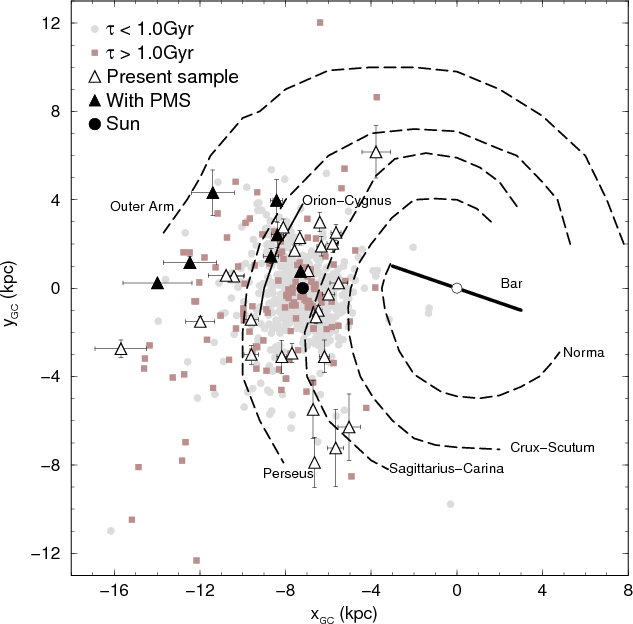
|
Figure 11: Schematic projection of the Galaxy, as seen from the North Pole, with 7.2 kpc as the Sun's distance to the Galactic centre, in which the projected distribution of the present Teutsch star clusters (triangles) is compared to the WEBDA OCs younger (circles) and older than 1 Gyr (squares). Clusters with PMS stars are shown as filled triangles. Main Galactic structures are identified. |
| Open with DEXTER | |
7.3 Relations with cluster size
Despite some scatter, a first-order dependence of cluster size on
Galactocentric distance shows up in Fig. 12 (panel a), similar
to what has already been observed by, e.g.
Lyngå (1982), Tadross et al. (2002),
and van den Bergh et al.
(1991). Although with more scatter, a similar relation occurs
for cluster size and height over the Galactic plane ![]() (panel b). Both relations are consistent with a lower frequency of
encounters with giant molecular clouds and the disk for OCs at large
Galactocentric distances and high
(panel b). Both relations are consistent with a lower frequency of
encounters with giant molecular clouds and the disk for OCs at large
Galactocentric distances and high ![]() ,
with respect to those orbiting in the inner Galaxy and/or closer to the
plane. However, part of the
,
with respect to those orbiting in the inner Galaxy and/or closer to the
plane. However, part of the ![]() relation may arise from differential completeness. Given that the
average background+foreground contamination decreases with increasing
relation may arise from differential completeness. Given that the
average background+foreground contamination decreases with increasing ![]() ,
the external parts of an OC (where the surface brightness is
intrinsically low) can be detected at larger distances (from the
cluster centre) for high-
,
the external parts of an OC (where the surface brightness is
intrinsically low) can be detected at larger distances (from the
cluster centre) for high-
![]() objects than for those near the plane (Bonatto
et al. 2006). Thus, on average, high-
objects than for those near the plane (Bonatto
et al. 2006). Thus, on average, high-
![]() clusters tend to seem bigger than those near the plane.
clusters tend to seem bigger than those near the plane.
|
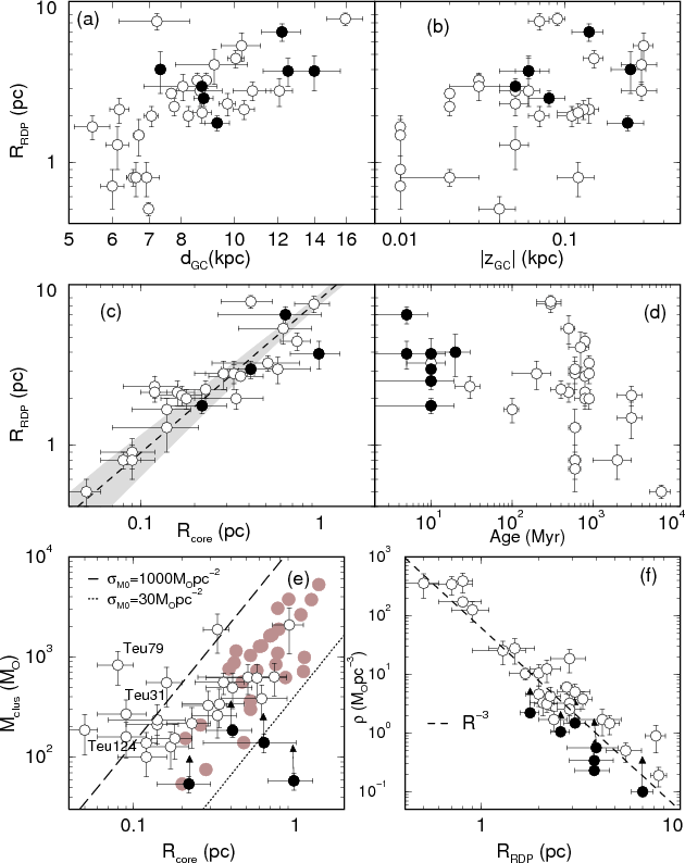
Figure 12:
Top: relation of the cluster radius with
Galactocentric distance ( left)
and distance from the plane ( right).
Middle left: cluster and core radii are related as |
| Open with DEXTER | |
|
Figure 13:
The integrated and reddening-corrected colours correlate (panel
a)) as
|
| Open with DEXTER | |
The relation between cluster radius and age, which is
intimately related to cluster survival/dissociation rates, is examined
in panel (d). While some of the clusters appear to expand as
they age, others seem to shrink, with a bifurcation occurring at ![]() 1 Gyr.
The same applies to the core radius, given the correlation between
1 Gyr.
The same applies to the core radius, given the correlation between ![]() and
and ![]() (c).
A similar relation of core radius with age has been observed by Mackey & Gilmore (2003)
in LMC and SMC star clusters. Mackey
& Gilmore (2008) attributed the slow
(c).
A similar relation of core radius with age has been observed by Mackey & Gilmore (2003)
in LMC and SMC star clusters. Mackey
& Gilmore (2008) attributed the slow ![]() contraction to dynamical relaxation and/or core collapse. The expansion
may come from stellar evolution-related mass loss in a mass-segregated
or centrally concentrated cluster, and from heating due to a
significant population of black holes that are scattered into the
cluster halo or ejected from the cluster (e.g. Mackey
et al. 2007; Merritt
et al. 2004).
contraction to dynamical relaxation and/or core collapse. The expansion
may come from stellar evolution-related mass loss in a mass-segregated
or centrally concentrated cluster, and from heating due to a
significant population of black holes that are scattered into the
cluster halo or ejected from the cluster (e.g. Mackey
et al. 2007; Merritt
et al. 2004).
Table 5: Integrated magnitude and colours.
As discussed in Bonatto & Bica (2009b), when the projected mass density of a star cluster follows a King-like profile (e.g. Bonatto & Bica 2008a), the cluster mass (Finally, we investigated the distribution of the Teutsch
clusters on the plane cluster radius and average mass density, ![]() vs.
vs. ![]() (panel f). The density decreases smoothly with cluster radius
- over the full radius (
(panel f). The density decreases smoothly with cluster radius
- over the full radius (
![]() )
and density (
)
and density (
![]() )
scales - as
)
scales - as ![]() ,
as for the sample of starburst clusters studied by Pfalzner (2009). Both
radius and density scales overlap those of the starburst and leaky
clusters of
Pfalzner (2009), which has
clusters more massive than
,
as for the sample of starburst clusters studied by Pfalzner (2009). Both
radius and density scales overlap those of the starburst and leaky
clusters of
Pfalzner (2009), which has
clusters more massive than ![]() and density within the very wide range
and density within the very wide range ![]() .
The boundary between starburst and leaky clusters occurs at
.
The boundary between starburst and leaky clusters occurs at ![]() pc
and
pc
and ![]() .
The
.
The ![]() dependence (in clusters younger than
dependence (in clusters younger than ![]() 20 Myr and more massive than
20 Myr and more massive than ![]()
![]() - Pfalzner 2009)
is taken as consequence of simple diffusion, in the sense that the
clusters expand without further mass loss (which would lead to a
steeper dependence, such as
- Pfalzner 2009)
is taken as consequence of simple diffusion, in the sense that the
clusters expand without further mass loss (which would lead to a
steeper dependence, such as ![]() ).
).
7.4 Integrated colours and magnitudes
The decontaminated photometry (Sect. 3) and structural
parameters (Sect. 5)
are used to compute the integrated (apparent and absolute) magnitudes
and reddening-corrected colours for the 2MASS bands. Since the
decontamination efficiency is lower than 100% (Sect. 3), we start by
applying the colour-magnitude filter to the decontaminated photometry.
Then we sum the flux (for a given band) of all stars within ![]() (Table 2)
to compute the cluster+residual field stars flux (
(Table 2)
to compute the cluster+residual field stars flux (
![]() ).
The same is
done for all the comparison field stars, to estimate the residual
contamination flux (
).
The same is
done for all the comparison field stars, to estimate the residual
contamination flux (
![]() ). Thus, the integrated
magnitude is given by
). Thus, the integrated
magnitude is given by ![]() ,
where
,
where ![]() is the ratio between the projected areas of the cluster and the
comparison field. This procedure is applied to the J,
H, and
is the ratio between the projected areas of the cluster and the
comparison field. This procedure is applied to the J,
H, and ![]() bands, and should minimise decontamination efficiency effects.
bands, and should minimise decontamination efficiency effects.
Since most of the evolved clusters contain giant and MSTO
stars (Figs. 1-6), which by far
dominate the luminosity, the integrated magnitudes should not be
significantly affected by not detecting the low-MS stars associated
with the depth-limited 2MASS photometry. Reddening and distance from
the Sun (for the absolute magnitude and reddening-corrected colours)
are those computed in Sect. 4,
and the results are given in Table 5. Figure 13 (panel a) shows
that the ![]() and
and ![]() colours are tightly correlated according to
colours are tightly correlated according to ![]() ,
so we can restrict the remaining analysis to
,
so we can restrict the remaining analysis to ![]() .
The reddening-corrected
.
The reddening-corrected ![]() colours are roughly distributed (b) around the average value
colours are roughly distributed (b) around the average value ![]() ,
with a
,
with a ![]() mag
spread. The absolute J magnitude distributes nearly
as a Gaussian around the average
value
mag
spread. The absolute J magnitude distributes nearly
as a Gaussian around the average
value ![]() ,
with a
,
with a ![]() 1.7 mag
standard deviation.
1.7 mag
standard deviation.
Finally, we use the relation between MV
and MJ, ![]() ,
derived for Galactic globular clusters by Bonatto
& Bica (2010b) to estimate the absolute V magnitude
of the Teutsch OCs. This relation was derived for the relatively wide
magnitude range
,
derived for Galactic globular clusters by Bonatto
& Bica (2010b) to estimate the absolute V magnitude
of the Teutsch OCs. This relation was derived for the relatively wide
magnitude range ![]() .
Extrapolating it
to the MJ
values derived for our Teutsch clusters, we find MV
values in the range
.
Extrapolating it
to the MJ
values derived for our Teutsch clusters, we find MV
values in the range ![]() (panel d of Fig. 13
and Table 5).
We now compare the Teutsch MV
values with those measured for 140 Galactic OCs (MWOCs) by Lata et al. (2002)
together with 106 OCs of Battinelli
et al. (1994)
(panel d of Fig. 13
and Table 5).
We now compare the Teutsch MV
values with those measured for 140 Galactic OCs (MWOCs) by Lata et al. (2002)
together with 106 OCs of Battinelli
et al. (1994)![]() .
Most (
.
Most (![]()
![]() )
of the MWOCs have MV
within
)
of the MWOCs have MV
within ![]() ,
but the remaining ones can be as luminous as
,
but the remaining ones can be as luminous as ![]() .
Clearly, our Teutsch clusters, in general, appear to be intrinsically
faint in the optical, with an MV
distribution somewhat biased to the low-luminosity tail of the MWOCs
distribution.
.
Clearly, our Teutsch clusters, in general, appear to be intrinsically
faint in the optical, with an MV
distribution somewhat biased to the low-luminosity tail of the MWOCs
distribution.
8 Summary and conclusions
In the present paper we have investigated the nature of 34 unstudied Teutsch clusters, and derived their astrophysical parameters. Distributed over all Galactic quadrants, we analysed them with field-star decontaminated 2MASS photometry that, by enhancing CMD evolutionary sequences and producing stellar RDPs that strongly contrast with the background, yields constrained astrophysical parameters. We could derive fundamental parameters for 33 objects, with the exception of (the apparently too distant) Teu 53.
Since the Teutsch clusters have been discovered in the
near-infrared, we derived
relatively high reddening values for some clusters, ![]() (or equivalently,
(or equivalently, ![]() ).
Also, about half of the sample is located more
distant than
).
Also, about half of the sample is located more
distant than ![]() kpc
from the Sun. The absolute J magnitudes distribute
around
kpc
from the Sun. The absolute J magnitudes distribute
around ![]() ,
while the MV
distribution is shifted about
2 mag towards fainter values. This suggests that our sample is
essentially
composed of low-luminosity clusters in the optical. In general, the
stellar
RDPs are highly contrasted with respect to the background and follow
the King-like
profile for most of the radial range. Cluster size correlates with
Galactocentric
distance and, to a lesser degree, with distance to the plane. Both
relations are
consistent with a low frequency of tidal stress (as well as low degree
of field
contamination), associated with large Galactocentric
distances and high-
,
while the MV
distribution is shifted about
2 mag towards fainter values. This suggests that our sample is
essentially
composed of low-luminosity clusters in the optical. In general, the
stellar
RDPs are highly contrasted with respect to the background and follow
the King-like
profile for most of the radial range. Cluster size correlates with
Galactocentric
distance and, to a lesser degree, with distance to the plane. Both
relations are
consistent with a low frequency of tidal stress (as well as low degree
of field
contamination), associated with large Galactocentric
distances and high-
![]() regions. We also found that the average mass density scales with
cluster radius as
regions. We also found that the average mass density scales with
cluster radius as ![]() .
In clusters younger than
.
In clusters younger than ![]() 20 Myr
and more massive than
20 Myr
and more massive than ![]()
![]() ,
this relation is typical of expansion by simple diffusion (Pfalzner 2009).
,
this relation is typical of expansion by simple diffusion (Pfalzner 2009).
With respect to the age, 8 clusters are younger than ![]() 30 Myr
(7 still hosting PMS stars), and 21 have ages within
100 Myr-900 Myr. Of particular interest is the
possibility of Teu 43, 50, and 77 having ages around
2-3 Gyr, while Teu 124 may be a significantly older
cluster, probably reaching
30 Myr
(7 still hosting PMS stars), and 21 have ages within
100 Myr-900 Myr. Of particular interest is the
possibility of Teu 43, 50, and 77 having ages around
2-3 Gyr, while Teu 124 may be a significantly older
cluster, probably reaching ![]() 7 Gyr.
7 Gyr.
Given the several dissolution mechanisms originating in its substructures, our Galaxy is a harsh environment for star clusters, especially the low-mass ones, to the point that most do not survive beyond a few 102 Myr. In this context, besides deriving astrophysical parameters for a significant sample of unstudied clusters, the main relevance of the present work lies in identifying open clusters older than several 102 Myr. In turn, an improved statistics on the population of clusters undergoing such evolved phases can be used to constrain the dissolution-time scale in the Galaxy.
AcknowledgementsWe thank an anonymous referee for interesting comments and suggestions. We acknowledge support from the Brazilian Institution CNPq. This publication makes use of data products from the Two Micron All Sky Survey, which is a joint project of the University of Massachusetts and the Infrared Processing and Analysis Center/California Institute of Technology, funded by the National Aeronautics and Space Administration and the National Science Foundation. This research made use of the WEBDA database, operated at the Institute for Astronomy of the University of Vienna. This research made use of NASA's Astrophysics Data System Service. This research has made use of the SIMBAD database, operated at the CDS, Strasbourg, France.
Appendix B: Metallicity estimate with Padovaisochrones
Our CMD analysis - and subsequent derivation of fundamental parameters
- is based on the updated set of Padova isochrones, whose distinctive
features are centred mostly on the greatly-improved treatment of the
thermally-pulsating asymptotic giant branch (TP-AGB) phase. The updated
isochrones preserve several peculiarities associated with the TP-AGB
tracks, i.e. the cool tails of C-type stars (by using proper molecular
opacities as convective dredge-up occurs along the TP-AGB), the
bell-shaped sequences in CMDs for stars with hot-bottom burning, the
pulsation mode changes between fundamental and first overtone, the
sudden changes in mean mass-loss rates as the surface chemistry changes
from M- to C-type, etc. (Marigo
et al. 2008). Isochrones are available for any age
within 0-17 Gyr,
metallicities within ![]() (
(
![]() ),
and masses in the range
),
and masses in the range ![]() .
We now discuss the possibility of using Padova isochrones and 2MASS
photometry to estimate metallicity.
.
We now discuss the possibility of using Padova isochrones and 2MASS
photometry to estimate metallicity.
As discussed by, e.g. Friel (2002, 1995), the location of a
given OC in the Galaxy seems to be more important for determining its
overall metallicity than the age. Indeed, both works show a nice trend
towards decreasing OC metallicity with increasing Galactocentric
distance. On the other hand, they also point to a lack of correlation
with cluster age. These works show that the observed OC metallicities,
in general, range from solar (
![]() ,
or Z=0.019) to sub solar (
,
or Z=0.019) to sub solar (
![]() ,
,
![]() )
values. A similar metallicity range is obtained when we consider the
observed metallicity gradient (Fig. 2 in
Friel 2002) coupled to the
derived Galactocentric distances of the present cluster sample
(Sect. 4).
)
values. A similar metallicity range is obtained when we consider the
observed metallicity gradient (Fig. 2 in
Friel 2002) coupled to the
derived Galactocentric distances of the present cluster sample
(Sect. 4).
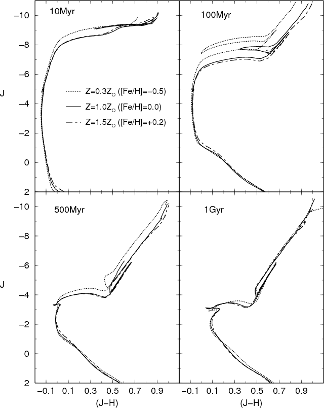
|
Figure B.1:
Comparison among Padova isochrones of different ages (10 Myr,
100 Myr, 500 Myr, and 1 Gyr) and
metallicities (
|
| Open with DEXTER | |
Considering the above, we compare in Fig. B.1 isochrones of
ages that characterise the values found for the present OCs
(Sect. 4)
and different metallicities. As the lower limit to the metallicity, we
use
![]() (Friel 2002), while for the
upper limit we take the
highest available Padova metallicity,
(Friel 2002), while for the
upper limit we take the
highest available Padova metallicity, ![]() .
.
The metal-rich isochrones are essentially indistinguishable in
the near infrared, while differences with respect to lower
metallicities are restricted to stars brighter than the MSTO and ages
younger than ![]() 500 Myr.
Basically, metal-poor isochrones present somewhat brighter (
500 Myr.
Basically, metal-poor isochrones present somewhat brighter (
![]() mag)
and bluer
(
mag)
and bluer
(
![]() mag)
giant clumps and red-giant branches. Thus, it is
difficult to assign a precise metallicity for poorly-populated clusters
(especially with respect to evolved stars), such as those dealt with in
this paper (Figs. 1-7).
mag)
giant clumps and red-giant branches. Thus, it is
difficult to assign a precise metallicity for poorly-populated clusters
(especially with respect to evolved stars), such as those dealt with in
this paper (Figs. 1-7).
References
- Allison, R. J., Goodwin, S. P., Parker, R. J., et al. 2009, ApJ, 700, L99
- Battinelli, P., Brandimarti, A., & Capuzzo-Dolcetta, R. 1994, A&AS, 104, 379
- Baumgardt, H., & Makino, J. 2003, MNRAS, 340, 227
- van den Bergh, S., Morbey, C., & Pazder, J. 1991, ApJ, 375, 594
- Bergond, G., Leon, S., & Guilbert, J. 2001, A&A, 377, 462
- Bessel, M. S., & Brett, J. M. 1988, PASP, 100, 1134
- Bica, E., Bonatto, C., & Camargo, D. 2008, MNRAS, 385, 349
- Bonatto, C., Bica, E., & Girardi, L. 2004, A&A, 415, 571
- Bonatto, C., Kerber, L. O., Bica, E., & Santiago, B. X. 2006, A&A, 446, 121
- Bonatto, C., & Bica, E. 2006, A&A, 455, 931
- Bonatto, C., & Bica, E. 2007a, A&A, 473, 445
- Bonatto, C., & Bica, E. 2007b, MNRAS, 377, 1301
- Bonatto, C., & Bica, E. 2008a, A&A, 477, 829
- Bonatto, C., & Bica, E. 2009a, MNRAS, 392, 483
- Bonatto, C., & Bica, E. 2009b, MNRAS, 394, 2127
- Bonatto, C., & Bica, E. 2009c, MNRAS, 397, 1915
- Bonatto, C., & Bica, E. 2010a, A&A, 516, A81
- Bonatto, C., & Bica, E. 2010b, MNRAS, 407, 1728
- Cardelli, J. A., Clayton, G. C., & Mathis, J. S. 1989, ApJ, 345, 245
- Dias, W. S., Alessi, B. S., Moitinho, A., & Lépine, J. R. D. 2002, A&A, 389, 871
- Drimmel, R., & Spergel, D. N. 2001, ApJ, 556, 181
- Dutra, C. M., Santiago, B. X., & Bica, E. 2002, A&A, 383, 219
- Elmegreen, B. G. 2008, in Globular Clusters - Guides to Galaxies, ESO Astrophysics Symposia (Berlin Heidelberg: Springer), 2009, 87
- Freudenreich, H. T. 1998, ApJ, 492, 495
- Friel, E. D. 1995, ARA&A, 33, 381
- Friel, E. D., Janes, K. A., Tavarez, M., et al. 2002, AJ, 124, 2693
- Girardi, L., Bertelli, G., Bressan, A., et al. 2002, A&A, 391, 195
- Goodwin, S. P., & Bastian, N. 2006, MNRAS, 373, 752
- Khalisi, E., Amaro-Seoane, P., & Spurzem, R. 2007, MNRAS, 374, 703
- King, I. 1962, AJ, 67, 471
- Kronberger, M., Teutsch, P., Alessi, B., et al. 2006, A&A, 447, 921
- Lada, C. J., & Lada, E. A. 2003, ARA&A, 41, 57
- Lamers, H. J. G. L. M., & Gieles, M. 2006, A&AL, 455, 17
- Lamers, H. J. G. L. M., Gieles, M., Bastian, N., et al. 2005, A&A, 441, 117
- Lata, S., Pandey, A. K., Sagar, R., & Mohan, V. 2002, A&A, 388, 158
- Lyngå, G. 1982, A&A, 109, 213
- Mackey, A. D., & Gilmore, G. F. 2003, MNRAS, 338, 120
- Mackey, A. D., Wilkinson, M. I., Davies, M. B., & Gilmore, G. F. 2007, MNRAS, 379, 40
- Mackey, A. D., Gilmore, G. F., Davies, M. B., & Gilmore, G. F. 2008, MNRAS, 386, 65
- Marigo, P., Girardi, L., Bressan, A., et al. 2008, A&A, 482, 883
- Merritt, D., Piatek, S., Portegies Zwart, S., & Hemsendorf, M. 2004, ApJ, 608, 25
- Momany, Y., Zaggia, S., Gilmore, G., et al. 2006, A&A, 451, 515
- Naylor, T., & Jeffries, R. D. 2006, MNRAS, 373, 1251
- Oort, J. H. 1958, in Ricerche Astronomiche, 5, 415, Specola Vaticana, Proc. of a Conference at Vatican Observatory, Castel Gandolfo, May 20-28, 1957, ed. D. J. K. O'Connell
- Pavani, D. N., & Bica, E. 2007, MNRAS, 468, 139
- Pfalzner, S. 2009 A&A, 498, 37
- Piskunov, A. E., Kharchenko, N. V., Röser, S., Schilbach, E., & Scholz, R.-D. 2006, A&A, 445, 545
- Piskunov, A. E., Schilbach, E., Kharchenko, N. V., Röser, S., & Scholz, R.-D. 2007, A&A, 468, 151
- Piskunov, A. E., Schilbach, E., Kharchenko, N. V., Röser, S., & Scholz, R.-D. 2008, A&A, 477, 165
- Russeil, D. 2003, A&A, 397, 133
- Skrutskie, M., Schneider, S. E., Stiening, R., et al. 1997, in The Impact of Large Scale Near-IR Sky Surveys, ed. F. Garzon, B. Burton, N. Epchtein, A. Omont, & P. Persi (Netherlands: Kluwer), 210, 187
- Spitzer, L. 1958, ApJ, 127, 17
- Tadross, A. L., Werner, P., Osman, A., & Marie, M. 2002, NewAst, 7, 553
- Trager, S. C., King, I. R., & Djorgovski, S. 1995, AJ, 109, 218
- Vallée, J. P. 2005, AJ, 130, 56
- Yadav, R. K. S., & Sagar, R. 2001, MNRAS, 328, 370
Online Material
Appendix A: LEDAS images
The images have been taken from LEDAS![]() ,
with a field of view adequate
to the angular dimension of each cluster. The same applies to the image
band. Information on field of view and image band can be read directly
on each image.
,
with a field of view adequate
to the angular dimension of each cluster. The same applies to the image
band. Information on field of view and image band can be read directly
on each image.
![\begin{figure}\par\mbox{\includegraphics[width=4.5cm]{Teu54.eps}\includegraphics...
...width=4.5cm]{Teu14a.eps}\includegraphics[width=4.5cm]{Teu13.eps} }\end{figure}](/articles/aa/full_html/2010/13/aa15222-10/img892.png)
|
Figure A.1: LEDAS images of the target clusters. From top to bottom and left to right: Teu 54, 40, 49, and 64; Teu 144, 11, 27, and 79; Teu 48, 52, 126, and 7; Teu 12, 66, 14a, and 13. |
| Open with DEXTER | |
![\begin{figure}\par\includegraphics[width=4.5cm]{Teu23.eps}\includegraphics[width...
...ics[width=4.5cm]{Teu45.eps}\includegraphics[width=4.5cm]{Teu39.eps}
\end{figure}](/articles/aa/full_html/2010/13/aa15222-10/img893.png)
|
Figure A.2: Same as Fig. A.1 for Teu 23, 76, 55, and 132; Teu 124, 60, 77, and 43; Teu 2, 28, 44, and 31; Teu 85, 106, 45, and 39. |
| Open with DEXTER | |
![\begin{figure}\par\mbox{\includegraphics[width=4.5cm]{Teu162.eps}\hspace*{9cm}
\includegraphics[width=4.5cm]{Teu53.eps} }
\par
\end{figure}](/articles/aa/full_html/2010/13/aa15222-10/img894.png)
|
Figure A.3: Same as Fig. A.1 for Teu 162 and 53. |
| Open with DEXTER | |
Footnotes
- ... clusters
- Appendix A is only available in electronic form at http://www.aanda.org
- ... WEBDA
- http://www.univie.ac.at/webda
- ... Candidates
- http://www.astro.iag.usp.br/wilton/
- ... photometry
- http://www.ipac.caltech.edu/2mass/releases/allsky/
- ... SIMBAD
- simbad.u-strasbg.fr/simbad/
- ... Candidates''
- http://www.astro.iag.usp.br/ wilton/
- ...
VizieR
- vizier.u-strasbg.fr/viz-bin/VizieR?-source=II/246
- ... regions
- This step is iterative, since we first build the RDP (Sect. 5) to estimate the cluster size and the location of the comparison field. After decontamination, we build the colour-magnitude filter, rebuild the RDP, recompute the cluster size, and repeat the decontamination.
- ... filters
- stev.oapd.inaf.it/cgi-bin/cmd
- ...
match
- In the sense that any isochrone solution that occurs within the photometric error bars is taken as acceptable.
- ... cluster
- They are wide enough to take photometric uncertainties and binaries into account (or other multiple systems).
- ...
feature
- Alternatively, clusters that form dynamically cool and with significant substructure will probably develop an irregular central region, unless such a region collapses and smooths out the initial substructure (Allison et al. 2009).
- ... MF
-
 for
for
 ,
,
 for
for
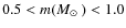 ,
and
,
and
 for
for
 .
.
- ...Battinelli et al. (1994)
- Both samples have similar MV distributions. For the OCs in common we used the more recent values of Lata et al. (2002).
- ... LEDAS
- Leicester Database and Archive Service (LEDAS) DSS/DSS-II service on ALBION; ledas-www.star.le.ac.uk/DSSimage.
All Tables
Table 1: Fundamental parameters.
Table 2: Structural parameters derived from the RDPs.
Table 3: Stellar mass estimate.
Table 4: Stellar mass estimate for the clusters with PMS.
Table 5: Integrated magnitude and colours.
All Figures
|
|
Figure 1: CMDs of Teu 54, 40, 49, 64, and 144 for a representative cluster region (top panels) and the equal-area comparison field (middle). The decontaminated CMDs (bottom) are shown with the isochrone solution (solid line) and the colour-magnitude filter (shaded polygon). |
| Open with DEXTER | |
| In the text | |
|
|
Figure 2: Same as Fig. 1 for Teu 11, 27, 79, 48, and 52. |
| Open with DEXTER | |
| In the text | |
|
|
Figure 3: Same as Fig. 1 for Teu 126, 7, 12, 66, and 14a. |
| Open with DEXTER | |
| In the text | |
|
|
Figure 4:
Same as Fig. 1
for Teu 13 ( left panel). The remaining
clusters
(Teu 23, 7, 76, 55, and 132) are shown in |
| Open with DEXTER | |
| In the text | |
|
|
Figure 5: Same as Fig. 1 for Teu 124, 50, 77, 43, and 2. Isochrones younger than the adopted ones are also shown for an estimate of a lower limit to the age. |
| Open with DEXTER | |
| In the text | |
|
|
Figure 6: Same as Fig. 1 for Teu 28, 44, 31, 85, and 106. |
| Open with DEXTER | |
| In the text | |
|
|
Figure 7:
Same as Fig. 1
but with |
| Open with DEXTER | |
| In the text | |
|
|
Figure 8:
Stellar RDPs (empty circles), the best-fit King-like profile (solid
line), the |
| Open with DEXTER | |
| In the text | |
|
|
Figure 9: Same as Fig. 8 for the remaining clusters. It was not possible to fit the King-like profile for some cases. |
| Open with DEXTER | |
| In the text | |
|
|
Figure 10: General properties of the present OCs (filled circles) compared to Galactic clusters (empty circles) taken from Dias et al. (2002) and WEBDA (panels a), b), and c)), and Piskunov et al. (2008) d). All cases are investigated with distribution functions. |
| Open with DEXTER | |
| In the text | |
|
|
Figure 11: Schematic projection of the Galaxy, as seen from the North Pole, with 7.2 kpc as the Sun's distance to the Galactic centre, in which the projected distribution of the present Teutsch star clusters (triangles) is compared to the WEBDA OCs younger (circles) and older than 1 Gyr (squares). Clusters with PMS stars are shown as filled triangles. Main Galactic structures are identified. |
| Open with DEXTER | |
| In the text | |
|
|
Figure 12:
Top: relation of the cluster radius with
Galactocentric distance ( left)
and distance from the plane ( right).
Middle left: cluster and core radii are related as |
| Open with DEXTER | |
| In the text | |
|
|
Figure 13:
The integrated and reddening-corrected colours correlate (panel
a)) as
|
| Open with DEXTER | |
| In the text | |
|
|
Figure B.1:
Comparison among Padova isochrones of different ages (10 Myr,
100 Myr, 500 Myr, and 1 Gyr) and
metallicities (
|
| Open with DEXTER | |
| In the text | |
|
|
Figure A.1: LEDAS images of the target clusters. From top to bottom and left to right: Teu 54, 40, 49, and 64; Teu 144, 11, 27, and 79; Teu 48, 52, 126, and 7; Teu 12, 66, 14a, and 13. |
| Open with DEXTER | |
| In the text | |
|
|
Figure A.2: Same as Fig. A.1 for Teu 23, 76, 55, and 132; Teu 124, 60, 77, and 43; Teu 2, 28, 44, and 31; Teu 85, 106, 45, and 39. |
| Open with DEXTER | |
| In the text | |
|
|
Figure A.3: Same as Fig. A.1 for Teu 162 and 53. |
| Open with DEXTER | |
| In the text | |
Copyright ESO 2010
Current usage metrics show cumulative count of Article Views (full-text article views including HTML views, PDF and ePub downloads, according to the available data) and Abstracts Views on Vision4Press platform.
Data correspond to usage on the plateform after 2015. The current usage metrics is available 48-96 hours after online publication and is updated daily on week days.
Initial download of the metrics may take a while.