| Issue |
A&A
Volume 521, October 2010
|
|
|---|---|---|
| Article Number | A25 | |
| Number of page(s) | 7 | |
| Section | Astrophysical processes | |
| DOI | https://doi.org/10.1051/0004-6361/201015210 | |
| Published online | 15 October 2010 | |
Potential vorticity dynamics in the framework of disk shallow-water theory
I. The Rossby wave instability
O. M. Umurhan1,2
1 - School of Mathematical Sciences, Queen Mary
University of London, London E1 4NS, UK
2 -
Astronomy Department, City College of San Francisco,
San Francisco, CA 94112, USA
Received 14 June 2010 / Accepted 13 July 2010
Abstract
Context. The Rossby wave instability in astrophysical disks
is a potentially important mechanism for driving angular momentum
transport in disks.
Aims. We attempt to more clearly understand this instability in
an approximate three-dimensional disk model environment which we assume
to be a single homentropic annular layer we analyze using disk
shallow-water theory.
Methods. We consider the normal mode stability analysis of two
kinds of radial profiles of the mean potential vorticity: the first
type is a single step and the second kind is a symmetrical step of
finite width describing either a localized depression or peak of the
mean potential vorticity.
Results. For single potential vorticity steps we find there is
no instability. There is no instability when the symmetric step is a
localized peak. However, the Rossby wave instability occurs when the
symmetrical step profile is a depression, which, in turn, corresponds
to localized peaks in the mean enthalpy profile. This is in qualitative
agreement with previous two-dimensional investigations of the
instability. For all potential vorticity depressions, instability
occurs for regions narrower than some maximum radial length scale. We
interpret the instability as resulting from the interaction of at least
two Rossby edgewaves.
Conclusions. We identify the Rossby wave instability in the
restricted three-dimensional framework of disk shallow water theory.
Additional examinations of generalized barotropic flows are needed.
Viewing disk vortical instabilities from the conceptual perspective of
interacting edgewaves can be useful.
Key words: hydrodynamics - accretion, accretion disks - instabilities
1 Introduction
The Rossby wave instability (hereafter RWI) is a promising candidate mechanism to account for the observed anomalous transport of cold astrophysical disksBecause of the potential importance of this mechanism for disks, it is worthwhile to consider and understand this instability in disk settings, which are three dimensional, at least in part. The goal of this study is to expose the machinery of this process as clearly as possible in the context of a three-dimensional theory.
Disk shallow water theory (Umurhan 2008, and hereafter DSW-theory) is a model reduction of the disk equations that is three-dimensional but asymptotic in the sense that azimuthal scales are much larger than the corresponding vertical and radial scales. It is essentially a model environment representing vortex dynamics occurring on thin annular sections of disks over timescales which are much longer than the local disk rotation time. The original motivation for this approximation was to develop a three-dimensional framework to describe the dynamics of elongated vortices known to emerge in two-dimensional studies such as that reported in Godon & Livio (1999). The benefit of using the DSW-theory is that it allows a transparent analysis of vortex dynamics free of other physical processes that are likely not to play a significant role - in particular, free of both acoustic and gravity mode oscillations. As such, by means of this framework one may develop a mechanical understanding of disk-related vortex dynamics.
In Umurhan (2008), DSW-theory was applied to understand the emergence of one form of the strato-rotational instability, which is an instability of a stably stratified Rayleigh stable shear profile in a channel (Yavneh 2001; Dubrulle et al. 2005). The no-normal flow boundary conditions at the walls of the domain bring into existence edgewaves (e.g., Goldreich et al. 1986) that propagate along the walls in opposite directions with respect to one another. However, because the edgewaves may also interact with one another across the domain, if the separation of the walls fall within a specific allowed range, then the phase speeds of the edgewaves can ``resonate'' with each other and become unstable (Umurhan 2006; Umurhan 2008).
This edgewave dynamical picture has been used to understand the development
of many forms of potential vorticity driven geophysical fluid instabilities including, among others,
the original problem considered by Rayleigh (Hoskins et al. 1985; Baines & Mitsudera 1994;
Heifetz et al. 1999)
as well as astrophysical processes such as
the Papaloizou-Pringle instability (Papaloizou & Pringle 1984; Goldreich et al. 1985).
In the geophysical fluid dynamics context, this is frequently referred to as
the instability of counter-propagating Rossby waves (e.g., Heifetz et al. 1999).
The use of edgewaves as an interpretive tool has precedence
in the analysis of plasma instabilities. For example, the diocotron effect,
which is an instability associated with finite thickness charge sheets subjected
to ![]() drift, is rationalized to arise from the interaction of
edgewaves counter-propagating along
the surfaces of the charge sheet (Knauer 1966).
drift, is rationalized to arise from the interaction of
edgewaves counter-propagating along
the surfaces of the charge sheet (Knauer 1966).
![\begin{figure}
\par\includegraphics[width=9cm,clip]{15120fg1.eps}
\end{figure}](/articles/aa/full_html/2010/13/aa15210-10/img11.png)
|
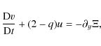
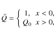
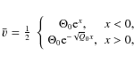
Figure 1:
Sketches of profile plots considered in this work. a) Single defect/jump located
at x=0. b) Double defect (symmetric step) with jumps located at
|
| Open with DEXTER | |
DSW-theory is an appropriate platform to examine the RWI. Indeed, an examination of the vortex structures emerging from nonlinear calculations of the instability (see Fig. 1 of Li et al. 2000, hereafter LFLC-2000) shows that the coherent vortex structure is severely elongated in the azimuthal direction while being radially tightly confined. This structural quality is similar to the vortices reported in Godon & Livio (1999). The advantage of DSW-theory is that it can capture some essence of three-dimensionality, while its disadvantage is that, because of its construction, small azimuthal scales cannot be represented. By contrast, the vertically integrated model environment used in the original RWI studies are able to capture small azimuthal scales while coming at the expense of representing three-dimensionality.
In this study, the RWI is examined in the framework of DSW-theory.
The stability of two analytically tractable mean PV-profiles is studied: (i)
a single defect, or ``single-step''; and (ii) a double defect, or ``symmetric-step''
(see Fig. 1).
As in the case of the stratorotational instability, the RWI
is shown to result from the interaction of Rossby edgewaves
that propagate along the locations of the steps of the mean PV-profile. However,
the instability manifests itself only in the symmetric step case.
In Sect. 2, the equations of motion
and their perturbations are presented. In Sect. 3, the equations are analyzed for
two kinds of mean potential vorticity profiles including the one just described.
Analytic solutions are determined
throughout by considering the quasi-linear problem posed by considering the special
case
![]() ,
where
,
where ![]() is the ratio of specific heats.
Section 4 concludes with comments and a discussion about
recent three-dimensional RWI calculations (Meheut et al. 2010).
is the ratio of specific heats.
Section 4 concludes with comments and a discussion about
recent three-dimensional RWI calculations (Meheut et al. 2010).
2 Equations and potential vorticity conservation
The asymptotic equations upon which DSW-theory is based, describing the evolution of annular
disk sections, was developed in Umurhan (2008). In that study, the equations
of motion for an annular section in which the vertical/radial extent ![]() is much smaller
that the azimuthal scale R was developed as an asymptotic series expansion in
powers of
is much smaller
that the azimuthal scale R was developed as an asymptotic series expansion in
powers of
![]() .
The timescales of
the dynamics (
.
The timescales of
the dynamics (![]() )
is comparatively long with respect
to the local rotation time (
)
is comparatively long with respect
to the local rotation time (
![]() )
of the annular disk centered
on R0 i.e.,
)
of the annular disk centered
on R0 i.e.,
![]() .
To ensure a non-trivial
asymptotic balance, the radial and vertical velocities viewed in the reference
frame of the annulus rotating with
.
To ensure a non-trivial
asymptotic balance, the radial and vertical velocities viewed in the reference
frame of the annulus rotating with ![]() must scale as
must scale as
![]() where
where
![]() is the sound speed of the gas, while the corresponding deviations of
the azimuthal velocities must scale as
is the sound speed of the gas, while the corresponding deviations of
the azimuthal velocities must scale as ![]() .
This disparity in aspect and velocity ratios
is an asymptotic description of azimuthally elongated slowly overturning
vortices. Furthermore, the reduced equations
of motion in the annular disk section possess quasi-geostrophic characteristics
familiar in meteorological
studies.
.
This disparity in aspect and velocity ratios
is an asymptotic description of azimuthally elongated slowly overturning
vortices. Furthermore, the reduced equations
of motion in the annular disk section possess quasi-geostrophic characteristics
familiar in meteorological
studies.
Single constant entropy layers are considered when the equation
of state is polytropic, i.e., it is assumed that
![]() everywhere at all times.
This corresponds to a situation in which the specific entropy inside, defined by
everywhere at all times.
This corresponds to a situation in which the specific entropy inside, defined by
![]() ,
is everywhere a constant. This homentropic layer is considered in the following.
If there are radial variations of the mean height of the disk (h), then
the vertically integrated entropy of the disk also exhibits radial variations even though
the specific entropy is constant.
This point is made to keep in mind how the equations analyzed here
compares to the vertically integrated two-dimensional equations studied in
Li et al. (2000).
,
is everywhere a constant. This homentropic layer is considered in the following.
If there are radial variations of the mean height of the disk (h), then
the vertically integrated entropy of the disk also exhibits radial variations even though
the specific entropy is constant.
This point is made to keep in mind how the equations analyzed here
compares to the vertically integrated two-dimensional equations studied in
Li et al. (2000).
After non-dimensionalizing all the quantities according to the above,
the leading order equations
describing the evolution of varicose disturbances
of a single constant specific entropy layer are


where x,y represent the non-dimensional radial and azimuthal coordinates and t is the non-dimensionalized time (Umurhan 2008). In this construction, all quantities appearing are functions of these two coordinates and time. The radial velocity is u. The total time derivative is
The background shear

|
(5) |
where h=h(x,y,t) corresponds to the height of the disk measured from the disk midplane. The height h is the position at which the enthalpy goes to zero in the constant (specific) entropy environment. Although
Equation (1) is the radial momentum balance equation but in this asymptotic limit it says that all perturbations are radially geostrophic. Equation (2) is the azimuthal momentum balance and, unlike the radial version, no geostrophic balance is implied. Equations (3) and (4) represent, respectively, the motion of the surface h and an equation of state for the gas (see below). In the derivation contained in Umurhan (2008), these two equations result from (i) exploiting the hydrostasy of perturbations at all times and (ii) an analysis of the energy equation, which makes use of the linear independence of powers of z.
The disk vertical velocity, though not explicitly appearing,
is odd symmetric with respect to the disk midplane because of the
assumed varicose symmetry of the disk response. In the development of
the DSW-theory its functional form is shown to be
![]() .
In the reduction leading to these equations only
.
In the reduction leading to these equations only
![]() appears as well as the explicit evaluation of the velocity
of the layer at the height z=h. Additional details are found in Umurhan (2008).
appears as well as the explicit evaluation of the velocity
of the layer at the height z=h. Additional details are found in Umurhan (2008).
The combination of these equations of motion leads to the conservation of potential vorticity Qgiven by
|
(6) |
The next section considers the fate of normal modes for potential vorticity (or ``PV'' for short) profiles in which there is either a single or a double defect in the steady PV profile
3 Analytical study
The analysis in this work considers the fate of disturbances where
![]() .
This
is chosen because the resulting equations, both steady and normal mode disturances, may
be analyzed without intensive use of numerical methods. General more realistic values of
.
This
is chosen because the resulting equations, both steady and normal mode disturances, may
be analyzed without intensive use of numerical methods. General more realistic values of
![]() require numerical evaluation of both the steady and time-depenedent state and
this will be reserved for a future study. For
require numerical evaluation of both the steady and time-depenedent state and
this will be reserved for a future study. For
![]() ,
the PV expression takes on
the quasi-linear form
,
the PV expression takes on
the quasi-linear form
|
(7) |
The following sections consider the two analytically tractable defect profiles and their normal mode responses.
3.1 Single defect
In this study, the term defect is used to indicate places where steps
occur in the mean PV-profile. The following simple single defect,
|
(8) |
is studied. The value of Q0 is constrained to be greater than zero. Solutions are sought that are bounded as
|
(9) |
on either side of x=0(and where q = 3/2 has been explicitly used). The particular boundary conditions for the profiles at infinity are (i)
|
(10) |
where
|
(11) |
This result may be read to mean that the mean height
|
(12) |
which means that the deviation velocity at x=0 is given by
Infinitesimal perturbations of this steady state are
introduced by writing for each dependent quantity
![]() ,
where F'(x,y,t) is small
compared to the basic state
,
where F'(x,y,t) is small
compared to the basic state ![]() .
This means that
the potential vorticity equation is
.
This means that
the potential vorticity equation is
![\begin{displaymath}\Bigl[\partial_t + (\bar v - 3x/2)\partial_y\Bigr] Q'
+ u' \frac{{\rm d}\bar Q}{{\rm d}x} = 0,
\end{displaymath}](/articles/aa/full_html/2010/13/aa15210-10/img53.png)
|
(13) |
where Q' is given as
Because
|
(14) |
and requiring that the two solutions coming in from either side of x=0 satisfy the requirement that the normal velocities u' are the same there.
Normal mode solutions of the form
![]() are assumed.
Solutions with c>0 correspond to waves that propagate in the forward y direction
and, correspondingly, in the negative y direction for c<0.
It follows that the solution for
are assumed.
Solutions with c>0 correspond to waves that propagate in the forward y direction
and, correspondingly, in the negative y direction for c<0.
It follows that the solution for ![]() ,
away from the two boundaries,
satisfying the condition that their amplitudes are equal at x=0and,
,
away from the two boundaries,
satisfying the condition that their amplitudes are equal at x=0and,
![]() as
as
![]() ,
is
,
is
|
(15) |
where A0 is an arbitrary constant. The requirement that the normal perturbation velocities, u', match at the defect location means ensuring that
![\begin{displaymath}\left[
\frac{(\bar v_0-c-3x/2)\partial_x\hat\Xi + 2\hat\Xi}{1...
...^2\bar \Xi}
\right]^{x\rightarrow 0^+}_{x\rightarrow 0^-} = 0.
\end{displaymath}](/articles/aa/full_html/2010/13/aa15210-10/img61.png)
|
(16) |
Satisfaction of this condition leads to an eigenvalue condition on the wavespeed c which, after some algebra, reduces to the simple form
For
3.2 Double defect: the symmetric step
This subsection is an analysis of a symmetrical defect pair. The previous section demonstrates how a single defect produces a single Rossby edgewave along the defect. For two defects, therefore, two Rossby edgewaves are expected and it is under these circumstances that instability may emerge according to the principles of interacting waves (Hayashi & Young 1985; Baines & Mitsudera 1994; Heifetz et al. 1999).
The mean PV-profile appropriate for a double symmetric defect
is
|
(18) |
where
|
(19) |
The value of
|
(20) |
It means that for 0<Q0<1, the enthalpy deviation is a peak or bump, while for Q0>1the enthalpy structure is a depression. The corresponding mean velocity deviations are

|
(21) |
Defining
A qualitative sketch of the mean states are depicted in Fig. 1.
Because there are two defects, individual edgewaves
propagate along each of them, which interact with
each other as well. A normal-mode analysis, as
executed in the previous section, is performed. The details
are presented in the Appendix. The resulting wavespeed csatisfies the relationship
where

|
|||
|
|||

|
and
4 Comments and discussion
It has been shown that the RWI is recovered in the framework of DSW-theory. The RWI emerges when the idealized symmetric-step mean (radial) potential-vorticity profile is a depression (or equivalently, when the mean radial enthalpy profile is a peak). However, single stepped mean PV profiles do not support the instability. The RWI is interpreted as being caused by the interaction of two Rossby-edgewaves propagating azimuthally along each defect of the symmetric step PV-profile. These types of dynamical processes are a generic feature of many vortical dynamics in geophysical flows. Below is a collection of comments about these results including comparisons between the results of this work and the original RWI studies:
1. A weakness of the analysis performed here is that an unrealistic
value of the ratio of specific heats was used: a value of
![]() places the fluid in a thermodynamic regime somewhere between a normal gas
and an incompressible fluid (the latter being
places the fluid in a thermodynamic regime somewhere between a normal gas
and an incompressible fluid (the latter being
![]() ,
Salby 1989).
The main reason for this choice
was to develop the analysis analytically as most other values of
,
Salby 1989).
The main reason for this choice
was to develop the analysis analytically as most other values of ![]() require numerical methods to study both the steady states and the perturbation evolution.
Among other things, developing analytical solutions are important for benchmarking future analyses for
more reasonable values of
require numerical methods to study both the steady states and the perturbation evolution.
Among other things, developing analytical solutions are important for benchmarking future analyses for
more reasonable values of ![]() .
But most of all, the analytical solutions offer
the most transparency in interpreting the results.
Preliminary calculations for realistic values of
.
But most of all, the analytical solutions offer
the most transparency in interpreting the results.
Preliminary calculations for realistic values of ![]() show that the main mechanical interpretations
and qualitative solutions, as well as conditions for onset, are not considerably altered.
This is the subject
of a study in preparation.
show that the main mechanical interpretations
and qualitative solutions, as well as conditions for onset, are not considerably altered.
This is the subject
of a study in preparation.
2. The limiting form of the DSW-theory used to study the RWI considers the response of a
single homentropic disk layer. In this picture, the mean vertical height
of the disk is a function of the radial coordinate, i.e.,
![]() .
Instability only occurs when the enthalpy of the disk layer (which is
.
Instability only occurs when the enthalpy of the disk layer (which is ![]()
![]() )
has a peaked structure. In LFLC-2000, the RWI is demonstrated in a vertically integrated model of
a disk. Similar in quality to the results here, instability occurs when there is a
peak in the mean radial pressure profile (or, relatedly, the surface density profile). In contrast, however, instability occurs
for constant specific entropy profiles. This might imply that these
results conflict with one another.
)
has a peaked structure. In LFLC-2000, the RWI is demonstrated in a vertically integrated model of
a disk. Similar in quality to the results here, instability occurs when there is a
peak in the mean radial pressure profile (or, relatedly, the surface density profile). In contrast, however, instability occurs
for constant specific entropy profiles. This might imply that these
results conflict with one another.
Because the disk model considered in LFLC-2000 is vertically integrated, all
of the fluid quantities considered there are also understood to be vertically integrated,
including the entropy. In the DSW-theory framework studied here, despite
the specific entropy being constant throughout the layer, its vertical integration
is not constant if the mean height of the disk is not uniform. That is to say
if one defines
as the vertically integrated specific entropy of the disk, then it is self-evident that
3. With respect to the last point, the version of the RWI uncovered in the analysis of the symmetric step is qualitatively similar to the homentropic Gaussian bump profile (``HGB'') considered in LFLC-2000, where HGB describes the quality of the radial dependence of the mean pressure. However, as stated above, the symmetric step profile studied in this work is effectively non-homentropic when viewed in terms of the vertically integrated disk model considered in Li et al. (2000). The symmetric step profile might, therefore, most closely correspond to a non-homentropic Gaussian bump profile (``NGB'') in the framework of the vertically integrated model of LFLC-2000. A NGB profile was examined in the nonlinear regime in Li et al. (2001), and, in a qualitative sense, its evolution was not found to differ considerably.
One may, therefore, reasonably compare the conditions in which the RWI
arises in the HGB setting to the instability arising here for the
symmetric-step profile. In the analysis presented in LFLC-2000, it was shown
that for the HGB profile a minimum amplitude in the pressure bump was required
for instability to occur. It was indicated in Fig. 9. of that study
that the minimum variation required
in the associated surface mass density for instability to occur, on a
radial scale similar to the thickness of the disk,
must be between approximately 10% to 20% (LFLC-2000).
According to this study,
for any given value of
0 <Q0 < 1, instability occurs
for
![]() .
This means that for a given
peak value of the midplane enthalpy there is a maximum width size beyond
which instability ceases. In this sense, the results here imply
that there is no minimum required amplitude of the
midplane enthalpy peak (and, consequently, the corresponding
associated surface density peak)
for instability to occur.
.
This means that for a given
peak value of the midplane enthalpy there is a maximum width size beyond
which instability ceases. In this sense, the results here imply
that there is no minimum required amplitude of the
midplane enthalpy peak (and, consequently, the corresponding
associated surface density peak)
for instability to occur.
This does not necessarily
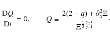
mean that these results disagree with each other. Indeed
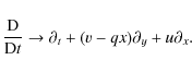
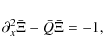
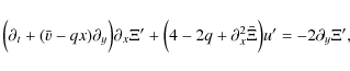
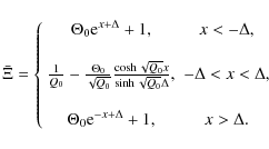
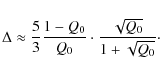
in Fig. 3, it can be seen that for fixed values of ![]() ,
there is a value of Q0 smaller than some critical value
for the system to be unstable. For example, for
,
there is a value of Q0 smaller than some critical value
for the system to be unstable. For example, for
![]() ,
instability occurs for Q0 < 0.5. According
to Fig. 2, this means that for
these parameter values the minimum midplane enthalpy peak variation
over the mean must be at least 25% for instability to occur.
,
instability occurs for Q0 < 0.5. According
to Fig. 2, this means that for
these parameter values the minimum midplane enthalpy peak variation
over the mean must be at least 25% for instability to occur.
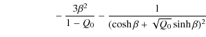
| Figure 2:
Plot of |
|
| Open with DEXTER | |
![\begin{figure}
\par\includegraphics[width=9cm,clip]{15120fg3.eps}
\end{figure}](/articles/aa/full_html/2010/13/aa15210-10/img95.png)
|
Figure 3:
Stability boundaries for the double defect problem in the
|
| Open with DEXTER | |
This still leaves open the question about the origin of the initial equilibrium.
In the general scenario proposed in LFLC-2000, matter is accumulated
in a piecemeal way, either by means of the coupling to large-scale magnetic field
processes or due to small-scale turbulence (possibility MHD driven). These
possibilities are not disputed here. Instead attention should be paid
to the way in which matter is accumulated. Reference to Fig. 3 best
illustrates this point. The way that matter accumulates
depends upn the path within the Q0-![]() plane along which the accumulation
process takes place. For example, if the process involves an increase in
plane along which the accumulation
process takes place. For example, if the process involves an increase in ![]() (the region size) for fixed values of 0<Q0<1, then instability will occur
before any sizeable enthalpy peak is reached
because any such path (starting from
(the region size) for fixed values of 0<Q0<1, then instability will occur
before any sizeable enthalpy peak is reached
because any such path (starting from
![]() )
is unstable to the RWI.
On the other hand, if the initial equilibrium Q0 is constructed on a path
of constant
)
is unstable to the RWI.
On the other hand, if the initial equilibrium Q0 is constructed on a path
of constant ![]() ,
then the system may be brought into the unstable regime
with a finite large amplitude of the enthalpy peak variation.
Thus, the way in which the equilibrium is constructed is crucial to assessing
how and on what scale the instability will operate. This point deserves further attention
in the future.
,
then the system may be brought into the unstable regime
with a finite large amplitude of the enthalpy peak variation.
Thus, the way in which the equilibrium is constructed is crucial to assessing
how and on what scale the instability will operate. This point deserves further attention
in the future.
4. The single step profile in the mean PV considered in this analysis shows no instability. In contrast, the single jump profiles studied in LFLC-2000 do show the emergence of instability. The reason for this difference is not entirely clear. One possibility is that the single step profile considered here may not be a faithful analog of the single jump profile studied in LFLC-2000. Indeed, in the generalized picture of edgewave dynamics of Baines & Mitsudera (1994), one needs a minimum of two edgewaves for instability to happen. The single-defect model of this study can only support a single edgewave and, therefore, no instability is possible. A corresponding analog representation of the single jump profile considered in LFLC-2000 probably needs to support at least two edgewaves in order to see the instability expressed. This is, however, conjecture at this stage and more analysis is needed.
5. Instability can be best rationalized in terms of the interaction of the two individual edgewaves propagating along each defect of the symmetric step profile. This picture is consistent with the Hayashi-Young criterion for wave instability (Hayashi & Young 1987), which can be summarized as follows: instability of two waves separated by an evanescent layer occurs when the two waves (i) propagate opposite to each other; (ii) have almost the same Doppler-shifted frequency; and (iii) can interact with one another. Interaction in this case means that the edgewave at one defect contributes to the perturbation velocity profile at the other defect.
All of these conditions for wave instability
are satisfied in the problem encountered here.
In particular,
one can view the Rossby-edgewaves propagating along each
defect as though they were disturbances
of isolated defects. Thus,
with respect
to the wavespeed calculation worked out for single isolated steps in PV
(Sect. 3.1), one can write down the wavespeeds associated
with each defect as
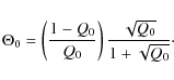
for the wave at
at
![\begin{figure}
\par\includegraphics[width=9cm,clip]{15120fg4.eps}\vspace*{-3.5mm}
\end{figure}](/articles/aa/full_html/2010/13/aa15210-10/img101.png)
|
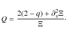
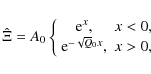
Figure 4:
wavespeeds as a function of |
| Open with DEXTER | |
In this particular double-defect setup it follows that one can roughly predict
the onset of instability to be when the isolated wavespeeds are
nearly zero in the reference frame of an observer at x=0. Using the
formula for ![]() given above,
given above,
![]() happens very nearly when
happens very nearly when
Clearly this can never happen when Q0 > 1 as

which is the same trend observed in Fig. 3.
The importance of this perspective is that one may approximately assess whether or not a more complicated looking PV-profile can become unstable to the RWI instability by appealing to this conceptually simple mechanistic view. For example, if a more sophisticated PV-profile were treated as if it were a series of PV-steps, then an approximate prediction for the onset of instability would only require calculating edgewave speeds along each defect taken as though each were in isolation. Onset conditions would be predicted for values of the parameters in which any two of these wavespeeds are nearly equal.
6. The asymptotic limit that the DSW-theory exploits is one in which
the azimuthal length scales are much longer than the radial ones. In this
limit there is no information as to how wavespeeds depend
upon the horizontal wavenumber ![]() .
In the theory developed here
the wavespeed c is independent of
.
In the theory developed here
the wavespeed c is independent of ![]() .
However, it is known that in
the vertically integrated configurations investigated in the original RWI studies
there is a clear dependence of c with
.
However, it is known that in
the vertically integrated configurations investigated in the original RWI studies
there is a clear dependence of c with ![]() .
.
On more concrete terms, in the numerical solution shown in LFLC-2000 there is
obviously
a fastest growing azimuthal wavenumber of the instability, which
leads to the final steady pattern state reached by the system. In contrast, in the
approximate study done here for the symmetric-step profile,
once stability is breached all wavenumbers become
unstable and there is no high-wavenumber cut off. The growth rates,
![]() ,
obviously increase without bound
in proportion to
,
obviously increase without bound
in proportion to ![]() - signaling the breakdown of the theory.
- signaling the breakdown of the theory.
To correct this issue, the DSW-theory would
have to be appropriately extended by allowing for
vertical structure in the horizontal velocities (i.e., inclusion of the
dependence ![]() z2) and some deviations from the linear dependenc
of the vertical velocity
with the z coordinate (i.e., an additional
z2) and some deviations from the linear dependenc
of the vertical velocity
with the z coordinate (i.e., an additional ![]() z3 dependency).
The resulting
next order correction to the
wavespeed in the extended DSW-theory
will show that the general dispersion relationship takes the form
z3 dependency).
The resulting
next order correction to the
wavespeed in the extended DSW-theory
will show that the general dispersion relationship takes the form
where
7. Three-dimensional numerical simulations of the RWI were announced during the preparation of this manuscript. Meheut et al. (2010) report on three-dimensional simulations of a constant entropy disk with midplane symmetric perturbations with the main goal of following the evolution of a Gaussian bump profile in the initial pressure field. Notable features of the results show that there is a significant amount of three-dimensional structure in the horizontal velocities as well as deviations from a linear z dependence of the vertical velocities. The resultant structures show interesting and complex three-dimensional structure in the streamlines of the flow. In contrast, in the asymptotic three-dimensional theory used here the horizontal velocities have no vertical variation and the vertical velocity is linear in z. Thus, the asymptotic strategy used here is far from matching the overall structure contained in the results of these particular simulations. The DSW-theory (or an analogous approach) may be extended to capture the quality of the dynamics contained in these numerical simulations much in line with the previous comments made in this regard. Moreover, it is important to understand how the three-dimensional structure emerges in these simulations, i.e., whether it arises from other secondary barotropic processes or if they are dynamics that are tied to the primary quasi-two dimensional dynamics driven by the primary instability. Rationalization of the three-dimensional dynamics in terms of the Rossby edgewave perspective utilized in this work could be a natural first step to this end.
AcknowledgementsThe author thanks Yiannis Tsapras, Oliver Gressel, Joe Barranco, and James Cho for discussions relating to this work. The author also thanks the anonymous referee for pointing out the analogy between the diocotron effect and the RWI. The author is indebted to the Kavli Institute of Theoretical Physics and the program Exoplanets Rising: Astronomy and Planetary Science at the Crossroads, where portions of this work were performed.
Appendix A: Double-defect normal-mode calculation
Following the procedure performed for the single defect, the equation Q' = 0 is solved separately in the three zones subject to the condition that
|
(A.1) |
while for

|
(A.2) |
The solution for

|
(A.3) |
The solution as presented satisfies the continuity of
![\begin{displaymath}\Bigg[
\frac{(\bar v(\Delta) - 3\Delta/2 -c)\partial_x\hat\Xi...
...i}
\Bigg]^{x\rightarrow \Delta^+}_{x\rightarrow \Delta^-} = 0,
\end{displaymath}](/articles/aa/full_html/2010/13/aa15210-10/img120.png)
|
(A.4) |
and
![\begin{displaymath}\Bigg[
\frac{(\bar v(-\Delta) + 3\Delta/2 -c)\partial_x\hat\X...
...
\Bigg]^{x\rightarrow -\Delta^+}_{x\rightarrow -\Delta^-} = 0.
\end{displaymath}](/articles/aa/full_html/2010/13/aa15210-10/img121.png)
|
(A.5) |
These two equations result in the matrix equation
where
References
- Baines, P. G., & Mitsudera, H. 1994, J. Fluid Mech., 276, 327 [NASA ADS] [CrossRef] [Google Scholar]
- Dubrulle, B., Marie, L. , Normand, Ch., et al. 2004, A&A, 429, 1 [Google Scholar]
- Friedman, B. 1956, Principles and Techniques of Applied Mathematics (New York: Wiley) [Google Scholar]
- Godon, P., & Livio, M. 1999, ApJ, 523, 350 [NASA ADS] [CrossRef] [Google Scholar]
- Goldreich, P., & Lynden-Bell, D. 1965, MNRAS, 130, 125 [NASA ADS] [CrossRef] [Google Scholar]
- Goldreich, P., Goodman, J., & Narayan, R. 1986, MNRAS, 221, 339 [NASA ADS] [Google Scholar]
- Hayashi, Y.-Y., & Young, W. R. 1987, J. Fluid Mech., 184, 477 [NASA ADS] [CrossRef] [Google Scholar]
- Heifetz, E., Bishop, C. H., & Alpert 1999, Q. J. R. Meteorol. Soc., 125, 2835 [NASA ADS] [CrossRef] [Google Scholar]
- Lovelace, R. V. E., & Hohlfeld, R. G. 1978, ApJ, 221, 51 [NASA ADS] [CrossRef] [Google Scholar]
- Hoskins, B. J., McIntyre, M. E., & Robertson, A. W. 1985, Q. J. R. Meteorol. Soc., 111, 877 [Google Scholar]
- Knauer, W. 1966, J. App. Phys., 37, 602 [Google Scholar]
- Li, H., Finn, J. M., Lovelace, R. V. E., & Colgate, S. A. 2000, LFLC-2000, ApJ, 533, 1023 [Google Scholar]
- Li, H., Colgate, S. A., Wendroff, B., & Liska R. 2001, ApJ, 551, 874 [NASA ADS] [CrossRef] [Google Scholar]
- Lovelace, R. V. E., Li, H., Colgate, S. A., & Nelson, A. F. 1999, ApJ, 513, 805 [NASA ADS] [CrossRef] [Google Scholar]
- Meheut, H., Casse, F., Varniere, P., & Tagger, M. 2010, A&A, 516, A31 [NASA ADS] [CrossRef] [EDP Sciences] [Google Scholar]
- Papaloizou, J. C. B., & Pringle, J. E. 1984, MNRAS, 208, 721 [NASA ADS] [CrossRef] [Google Scholar]
- Pedlosky, J. 1987, Geophysical Fluid Dynamics, 2nd edn. (New York: Springer-Verlag) [Google Scholar]
- Lord Rayleigh 1880, Proc. Royal Math. Soc., 9, 57 [Google Scholar]
- Salby, M. L. 1989, Tellus, 41A, 48 [NASA ADS] [CrossRef] [Google Scholar]
- Umurhan, O. M. 2006, MNRAS, 365, 85 [NASA ADS] [CrossRef] [Google Scholar]
- Umurhan, O. M. 2008, A&A, 489, 953 [NASA ADS] [CrossRef] [EDP Sciences] [Google Scholar]
- Yavneh I., McWilliams J. C., & Molemaker M. J. 2001 J. Fluid Mech., 448, 1 [Google Scholar]
Footnotes
- ... disks
![[*]](/icons/foot_motif.png)
- I.e., non-magnetized disks.
- ...
disk
- Note that in Lovelace & Hohlfeld (1978) the associated quantity f(r) corresponds roughly to the inverse of the PV.
- ...
- The single wavespeed formula
quoted above for c-is written in terms of the formula given in
Eq. (17) augmented by
the Doppler-shift consistent with the the local Keplerian
speed at
 .
The isolated edge wavespeed c+ is
correspondingly written taking into consideration
the symmetry of the mean PV-profile as viewed at
.
The isolated edge wavespeed c+ is
correspondingly written taking into consideration
the symmetry of the mean PV-profile as viewed at  ,
which
is the opposite of that at .
,
which
is the opposite of that at .
All Figures
|
|
Figure 1:
Sketches of profile plots considered in this work. a) Single defect/jump located
at x=0. b) Double defect (symmetric step) with jumps located at
|
| Open with DEXTER | |
| In the text | |
| |
Figure 2:
Plot of |
| Open with DEXTER | |
| In the text | |
|
|
Figure 3:
Stability boundaries for the double defect problem in the
|
| Open with DEXTER | |
| In the text | |
|
|
Figure 4:
wavespeeds as a function of |
| Open with DEXTER | |
| In the text | |
Copyright ESO 2010
Current usage metrics show cumulative count of Article Views (full-text article views including HTML views, PDF and ePub downloads, according to the available data) and Abstracts Views on Vision4Press platform.
Data correspond to usage on the plateform after 2015. The current usage metrics is available 48-96 hours after online publication and is updated daily on week days.
Initial download of the metrics may take a while.